1

Chapter 24

Electric Potential

Prof. Raymond Lee,revised 1-27-2013

2

• Electrical potential energy U

• If a test charge q0 is put in electric field E,

then q0 experiences a force F = q0E

• This force is conservative (i.e., path-

independent)

• ds is an infinitesimal displacement vector

oriented tangent to any spatial path

3

• Electric U, 2

• Work done by E-field is F•ds = q0E•ds

• As field does this work, charge-field

system’s potential energy U changes by

!U = -q0E•ds

• For finite displacement of charge from

A"B,

(Eqs. 24-17 & 24-18, p. 633)

4

• Electric U, 3

• Since q0E is conservative, line integral

doesn’t depend on charge’s path

• Thus !U = change in system’s PE

5

• Electric potential V

• PE per unit charge U/q0 is the electric

potential, which is:

• independent of q0’s value

• defined at every point in an E-field

• Define electric potential V = U/q0

6

• Electric V, 2

• V is a scalar quantity since energy is a

scalar

• As a charged particle moves in an E-

field, it experiences change in potential

(Eq. 24-18, p. 633)

7

• Electric V, 3

• Only V differences (i.e., !V) are meaningful

• We often set V = 0 at some convenientreference point in E-field

• V is a scalar characteristic of an E-field,independent of any test charges in that field

8

• Work & electric V

• Assume a charge q is moved in an E-

field without changing charge’s KE

• Then work Wapp done by an external

agent on charge q is: Wapp = !U = q !V(Eqs. 24-13 & 24-14, p. 631)

• Contrast this with work W done by field

itself on charge q: W = –!U = –q !V(Eq. 24-1, p. 628)

9

• Units of !V

• 1 V = 1 J/C (Eq. 24-9, p. 630)

• V is a volt

• 1 joule of work is needed to move a 1-C chargethrough a !V = 1 volt

• Also, 1 N/C = 1 V/m {= 1 J/(C*m) = 1 N*m/(C*m)}(see Eq. 24-10, p. 630)

• Can interpret E-field as measure of spatialgradient of V

10

• Electron volt

• An energy unit commonly used in atomic &

nuclear physics is electron-volt (eV)

• 1 eV is energy that a charge-field system

gains or loses when a charge of |e| (electron

or proton) moves through !V = 1 volt

• So 1 eV = 1.60 x 10-19 C•(1V) = 1.60 x 10-19 J

since 1 J = 1 C•V (see p. 630)

11

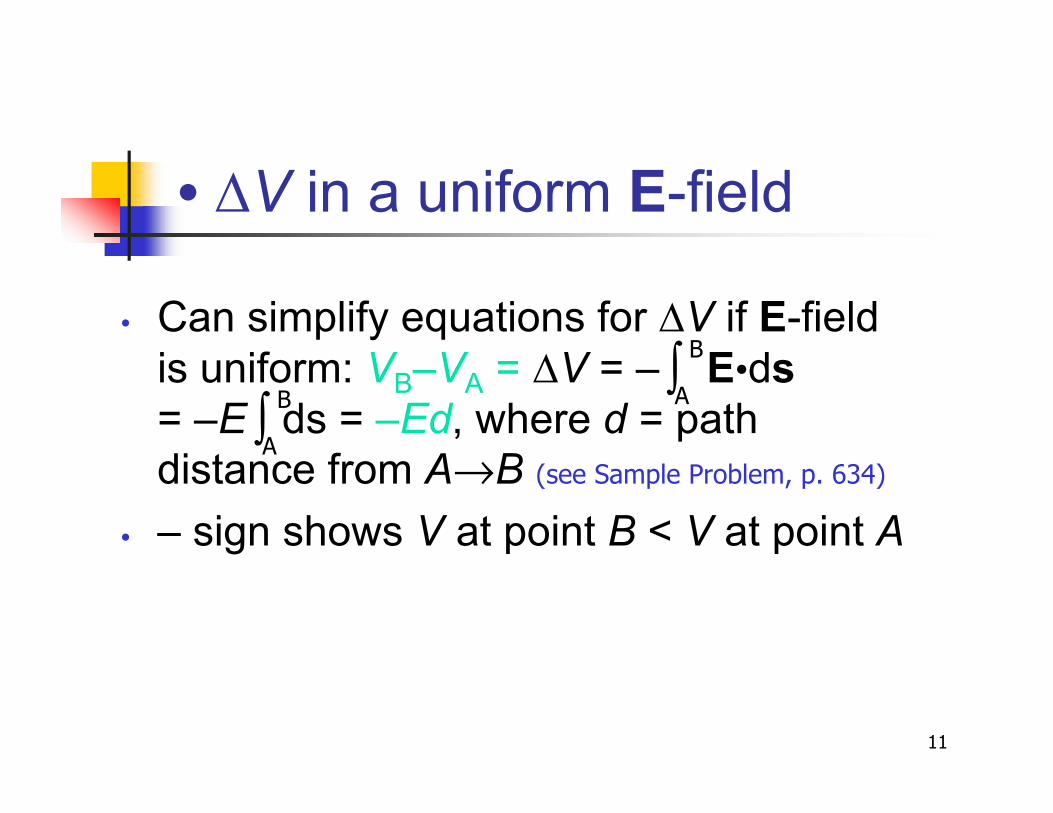
• !V in a uniform E-field

• Can simplify equations for !V if E-field

is uniform: VB–VA = !V = – E•ds

= –E ds = –Ed, where d = path

distance from A"B (see Sample Problem, p. 634)

• – sign shows V at point B < V at point A

#B

A

#B

A

12

• Energy & E-field direction

• When E-field points $, point

B is at lower V than point A

• If a +test charge moves fromA"B, then charge-field

system loses PE (i.e., !V < 0)

(SJ 2008Fig. 25.2,p. 695)

13

• Energy & E-field direction, 2

• System of +q0 & E-field loses electric U (i.e.,!U < 0) when +q0 moves with field

• True since E-field does work on +q0 when itmoves with field

• A moving +q0 gains KE = PE lost by charge-field system (i.e., energy conservation)

14

• Energy & E-field direction, 3

• If q0 is –, then !U > 0

• System consisting of –q0 & E-field gains

U when –q0 moves in field’s direction

• For –q0 to move with E-field, external

agent must do +work on the charge

15

• Equipotentials

• Point B is at lower V than

point A

• Points B & C are at same V

• An equipotential surface is

any surface with continuous

distribution of points at

constant V

(compare Fig. 24-5, p. 634)

16

• Charged particle in uniform E-field

• +q0 is released from rest& moves with E-field

• Then !V < 0 & !U < 0

• Fe & a on +q0 are in E-field’s direction

(SJ 2008 Fig. 25.6, p. 696)

17

• !V & point charges

• +point charge " E-field

pointing radially outward

• Then !V from A"B is:

(SJ 2008 Eq. 25.10, p. 697)

18

• !V & point charges, 2

• !V is independent of A"B path

• Pick reference V = 0 at rA = %

• Then V at point r is V = keq/r(Eq. 24-26, p. 635)

19

• V for a point charge

• Consider V in plane around

a point charge

• Red line shows V ’s 1/rdependence

(compare Fig. 24-7, p. 635)

20

• V for multiple charges

• Net V from several point charges is & ofVs from individual charges (superpositionprinciple)

• Then (Eq. 24-27, p. 636)

where V = 0 at reference distance r = %

21

• V for a dipole

• Consider V for an electric

dipole (along y-axis)

• Steep slope between +/-

charges shows strong

E-field here

• V = ke*p*cos(')/r2 where

' = angle from dipole axis(Eq. 24-30, p. 638) (SJ 2008 Fig. 25.8, p. 698)

22

• E & V for infinite sheet of charge

• Equipotential lines are

dashed blue lines

• E-field lines are brown lines

• Note equipotential lines are

everywhere ( E-field lines

(SJ 2008 Fig. 25.12, p. 701)

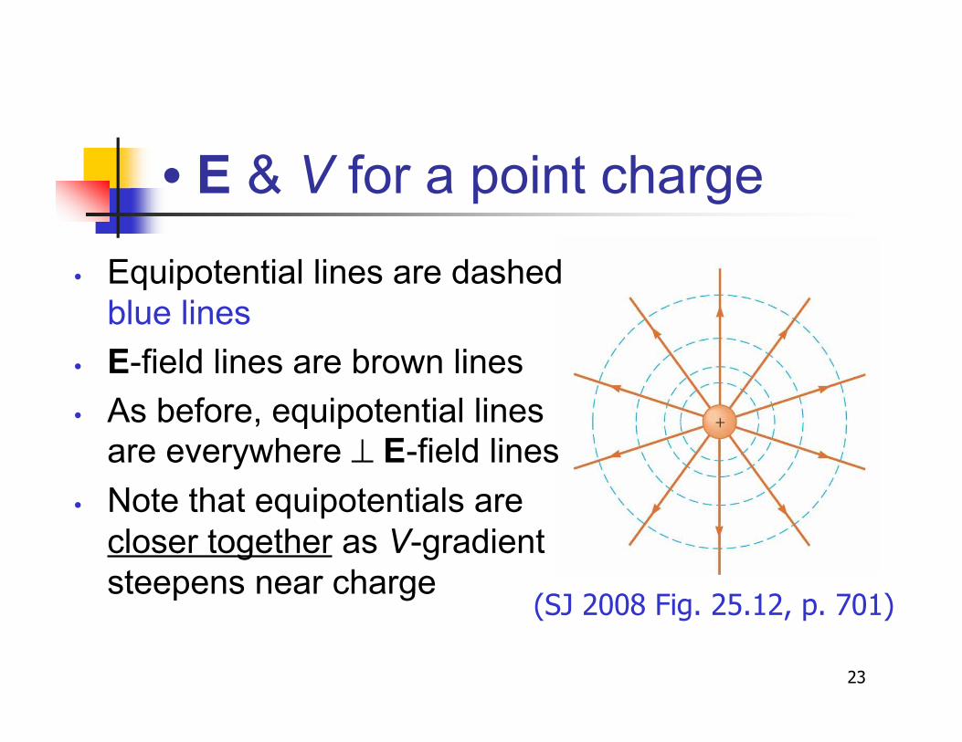
23

• E & V for a point charge

• Equipotential lines are dashed

blue lines

• E-field lines are brown lines

• As before, equipotential lines

are everywhere ( E-field lines

• Note that equipotentials are

closer together as V-gradient

steepens near charge(SJ 2008 Fig. 25.12, p. 701)

24

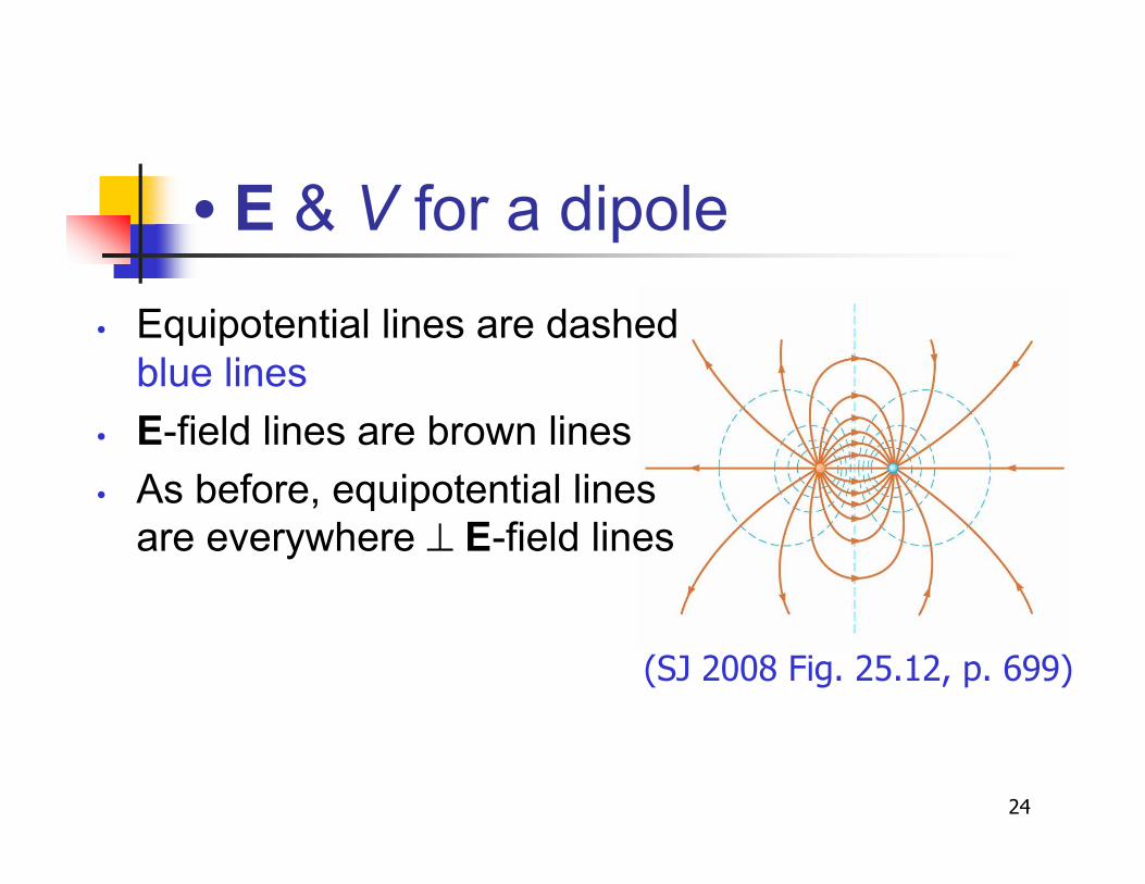
• E & V for a dipole

• Equipotential lines are dashed

blue lines

• E-field lines are brown lines

• As before, equipotential lines

are everywhere ( E-field lines

(SJ 2008 Fig. 25.12, p. 699)

25

• V for continuous charge distribution

• Treat small charge element dq

as a point charge on an object

of finite size & arbitrary shape

• Then potential dV at any point

due to dq is dV = kedq/r(Eq. 24-31, p. 639)

(SJ 2008 Fig. 25.14, p. 703)

26

• V for continuous charge distribution, 2

• To find total V, must integrate to include

contributions from all elements dq:

V = ke #dq/r (Eq. 24-32, p. 639)

• assumes reference value V(r =%) = 0 for

P infinitely far away from charged object

27

• V for a uniformly charged ring

• P is on ( central axis of

uniformly charged ring of

radius a & total charge Q

(SJ 2008 Fig.25.15, p. 704)

(SJ 2008 Eq. 25.21, p. 705)

28

• V for a uniformly charged disk

• Ring of radius a &surface charge density !

(compare Fig. 24-13, p. 640)

(compare Eq. 24-37, p. 640)

29

• V for finite line of charge

• Rod of length l has

total charge Q & linearcharge density "

(compare Fig.24-12, p. 639)

(compare Eq. 24-35, p. 640)

30

• V for uniformly charged sphere

• Solid insulating sphere of radius

R & total charge Q

• For r > R, V = keQ/r

• For r < R {e.g., inner radius D},

VD = keQ(3–r2/R2)

2R

(SJ 2004 Fig. 25.19, p. 777)

31

• V for uniformly charged sphere, 2

• Parabolic VD curve is forpotential inside sphere, & itsmoothly joins VB curve

• Note that ED = keQr/R3, justas found earlier

• Hyperbolic VB curve is forpotential outside sphere

(SJ 2004 Fig.25.20, p. 777)

32

• Finding E from V

• Assume E has only an x-component, so that

Ex = – dV/dx (Eq. 24-41, p. 641)

• Similar statements apply to Ey & Ez components

• Equipotential surfaces are always ( E-field linespassing through them

33

• E-field from V, general

• In general, V varies in all 3 dimensions

• Given V(x,y,z), you can find Ex, Ey, & Ez

as partial derivatives of V:

(Eq. 24-41, p. 641)

34

• U for multiple charges

• For 2 charged particles, system’s

PE (or U) is U = keq1q2/r12

(see Eq. 24-43, p. 643)

• If 2 charges have same sign,

U > 0 & must do work to bringthem together (i.e., to ) U)

• If 2 charges have opposite signs,

U < 0 & must do work to movethem apart () U again)

35

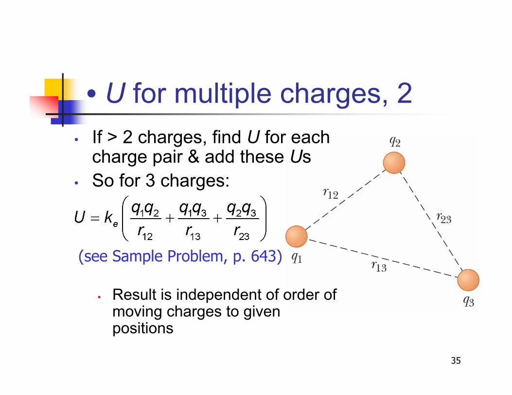
• U for multiple charges, 2

• If > 2 charges, find U for eachcharge pair & add these Us

• So for 3 charges:

• Result is independent of order ofmoving charges to givenpositions

(see Sample Problem, p. 643)

36

• V from charged conductor

• Consider 2 points A & B on surface ofarbitrary charged conductor

• E = 0 inside conductor & onconductor’s surface, have E ( surface

• Thus always have E ( displacementds along surface, so E•ds = 0

• As a result, !V between A & B = 0

(SJ 2008 Fig. 25.18, p. 707)

37

• V from charged conductor, 2

• V = constant everywhere on surface of chargedconductor in equilibrium (i.e., !V = 0 betweenany 2 points on surface)

• Surface of any charged conductor inelectrostatic equilibrium is equipotential surface

• Since E = 0 inside conductor, we know thatV = Vsurface (a constant) throughout interior

38

• E compared to V

• V(r) * 1/r, but E(r) * 1/r 2

• In space surrounding a charge, itsets up:• vector E-field related to force

• scalar potential V related to energy

V(r) & E(r) for conducting sphere (SJ 2008 Fig. 25.19, p. 707)

39

• Irregularly shaped objects

• Charge density + is high where

radius of curvature is small & low

where radius of curvature is large

• Model conductor as collection of

point charges with E(r) = keq/r 2

• So for nearby uncharged surfaces,distance r to conductor variesmore for its small-curvature parts

• E-field is large near convex points

with small radii of curvature & is

largest at sharp points (SJ 2004 Fig. 25.23, p. 779)

40

• Irregularly shaped objects, 2

• E-field lines are everywhere ( conducting surface

• Equipotential surfaces are everywhere ( E-field

lines

(SJ 2004 Fig.25.24, p. 779)

41

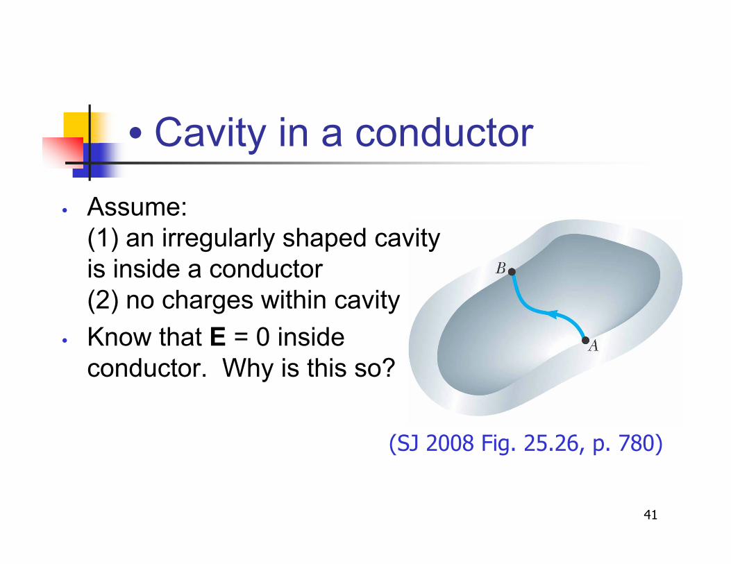
• Cavity in a conductor

(SJ 2008 Fig. 25.26, p. 780)

• Assume:

(1) an irregularly shaped cavity

is inside a conductor

(2) no charges within cavity

• Know that E = 0 inside

conductor. Why is this so?

42

• Cavity in a conductor, 2

• E-field inside doesn’t depend on chargedistribution on conductor’s exterior

• For all paths between points A & B, potential

difference VB–VA = – E•ds = 0 (i.e., all points

on conductor’s cavity wall are at same V)

• Since this holds for all paths on inner wall,must have E = 0 N/C everywhere inside cavity

• Thus a cavity with (a) conducting walls &(b) no enclosed charges is a field-free region

#B

A

43

• Corona discharge

• If E-field near a conductor is large, free

electrons from random ionizations of air

molecules accelerate away from these

“parent” molecules

• These free electrons

can ionize additional

molecules near

conductor

60 kV Tesla coil discharge

44

• Corona discharge, 2

• This " more free electrons

• Corona discharge is glow that resultsfrom recombination of these freeelectrons with ionized air molecules

• Ionization & corona discharge are mostlikely to occur near very sharp pointswhere + is largest

45

46

Millikan Oil-Drop Experiment –

Experimental Set-Up

47

Millikan Oil-Drop Experiment

, Robert Millikan measured e, the

magnitude of the elementary charge on

the electron

, He also demonstrated the quantized

nature of this charge

, Oil droplets pass through a small hole &

are illuminated by a light

48

Oil-Drop Experiment, 2

, With no electric field

between the plates,

the gravitational

force & the drag

force (viscous) act

on the electron

, The drop reaches

terminal velocity with

FD = mg

49

Oil-Drop Experiment, 3

, When an electric fieldis set up between theplates, The upper plate has a

higher potential

, The drop reaches anew terminal velocitywhen the electricalforce equals the sumof the drag force &gravity

50

Oil-Drop Experiment, final

, The drop can be raised & allowed to fall

numerous times by turning the electric

field on & off

, After many experiments, Millikan

determined:

, q = ne where n = 1, 2, 3, …

, e = 1.60 x 10-19 C

51

Van de Graaff

Generator

, Charge is delivered continuously toa high-potential electrode by meansof a moving belt of insulatingmaterial

, The high-voltage electrode is ahollow metal dome mounted on aninsulated column

, Large potentials can be developedby repeated trips of the belt

, Protons accelerated through suchlarge potentials receive enoughenergy to initiate nuclear reactions

52

Electrostatic Precipitator

, An application of electrical discharge in

gases is the electrostatic precipitator

, It removes particulate matter from

combustible gases

, The air to be cleaned enters the duct &

moves near the wire

, As the electrons & negative ions created by

the discharge are accelerated toward the

outer wall by the electric field, the dirt

particles become charged

, Most of the dirt particles are negatively

charged & are drawn to the walls by the

electric field

53

Application – Xerographic

Copiers

, The process of xerography is used for

making photocopies

, Uses photoconductive materials

, A photoconductive material is a poor

conductor of electricity in the dark but

becomes a good electric conductor when

exposed to light

54

The Xerographic Process

55

Application – Laser Printer

, The steps for producing a document on a laserprinter is similar to the steps in the xerographicprocess, Steps a, c, & d are the same

, The major difference is the way the image forms onthe selenium-coated drum

, A rotating mirror inside the printer causes the beam of thelaser to sweep across the selenium-coated drum

, The electrical signals form the desired letter in positivecharges on the selenium-coated drum

, Toner is applied & the process continues as in thexerographic process

56

Potentials Due to Various

Charge Distributions