chapter 21
DESCRIPTION
Chapter 21. Demand and Supply Elasticity. The evidence shows that an increase in the price of physician’s services or prescription medications results in a relatively small decrease in the quantity of these goods demanded. - PowerPoint PPT PresentationTRANSCRIPT
Chapter 21
Demand and Supply Elasticity

Slide 21-2
Introduction
The evidence shows that an increase in the price of physician’s services or prescription
medications results in a relatively small decrease in the quantity of these goods demanded.
In contrast, an increase in the price of psychiatric services causes a significant reduction in the
quantity demanded. Why is there a difference in the price responsiveness of these goods?

Slide 21-3
Learning Objectives
Express and calculate price elasticity of demand
Understand the relationship between the price elasticity of demand and total revenues
Discuss the factors that determine the price elasticity of demand

Slide 21-4
Learning Objectives
Describe the cross price elasticity of demand and how it may be used to indicate whether two goods are substitutes or complements
Explain the income elasticity of demand

Slide 21-5
Learning Objectives
Classify supply elasticities and explain how the length of time for adjustment affects the price elasticity of supply

Slide 21-6
Price Elasticity
Price Elasticity Ranges
Elasticity and Total Revenues
Determinants of the Price Elasticity of Demand
Chapter Outline

Slide 21-7
Chapter Outline
Cross Price Elasticity of Demand
Income Elasticity of Demand
Elasticity of Supply

Slide 21-8
Did You Know That...
Lower beer prices are associated with an increase in the number of violent incidents on campus?
A reduction in the price of a good can cause either an increase or a decrease in total sales revenue collected?

Slide 21-9
Price Elasticity
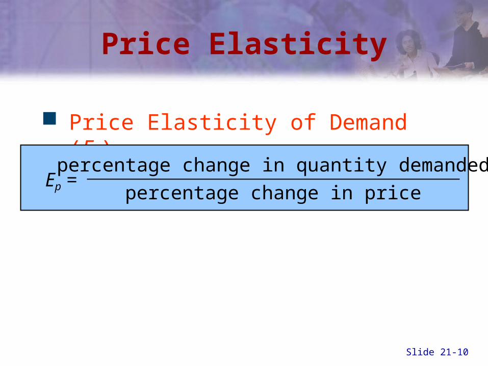
Price Elasticity of Demand (Ep)
– The responsiveness of quantity demanded of a commodity to changes in its price
Slide 21-10
Price Elasticity
Price Elasticity of Demand (Ep)
Ep = percentage change in quantity demanded
percentage change in price

Slide 21-11
Price Elasticity
Example
– Price of oil increases 10 percent
– Quantity demanded decreases 1 percent
Ep = -1%
+10%= -.1

Slide 21-12
Price Elasticity
Question
– How would you interpret an elasticity of -0.1?
Answer
– A ten percent increase in the price of oil will lead to a one percent decrease in quantity demanded

Slide 21-13
Price Elasticity
Relative quantities only
– Elasticity is measuring the change in quantity relative to the change in price
Always negative
– An increase in price decreases the quantity demanded, ceteris paribus

Slide 21-14
Calculating Elasticity
Elasticity formula:
change in Q
sum of quantities/2Ep =
change in P
sum of quantities/2
orchange in Q
(Q1 + Q2)/2Ep =
change in P
(P1 + P2)/2
Slide 21-15
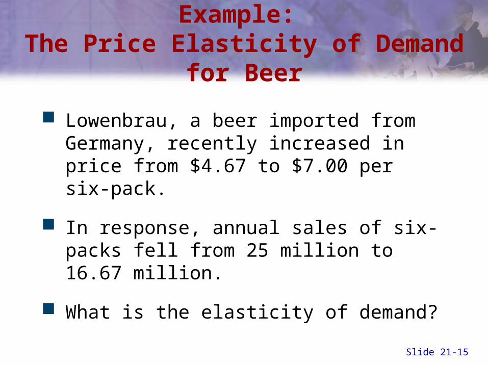
Example: The Price Elasticity of Demand for Beer
Lowenbrau, a beer imported from Germany, recently increased in price from $4.67 to $7.00 per six-pack.
In response, annual sales of six-packs fell from 25 million to 16.67 million.
What is the elasticity of demand?

Slide 21-16
Example: The Price Elasticity of Demand for Beer
Use the elasticity formula:
25-16.67 ÷ $7.00 – 4.67 (25 + 16.67)/2 ($7.00 +$4.67)/2
Solve the formula, and you will find that elasticity equals 1.

Slide 21-17
Price Elasticity Ranges
Elastic Demand
– Percentage change in quantity demanded is larger than the percentage change in price
– Ep > 1

Slide 21-18
Price Elasticity Ranges
Unit Elasticity of Demand
– Percentage change in quantity demanded is equal to the percentage change in price
– Ep = 1

Slide 21-19
Price Elasticity Ranges
Inelastic Demand
– Percentage change in quantity demanded is smaller than the percentage change in price
– Ep < 1
Slide 21-20
Price Elasticity Ranges
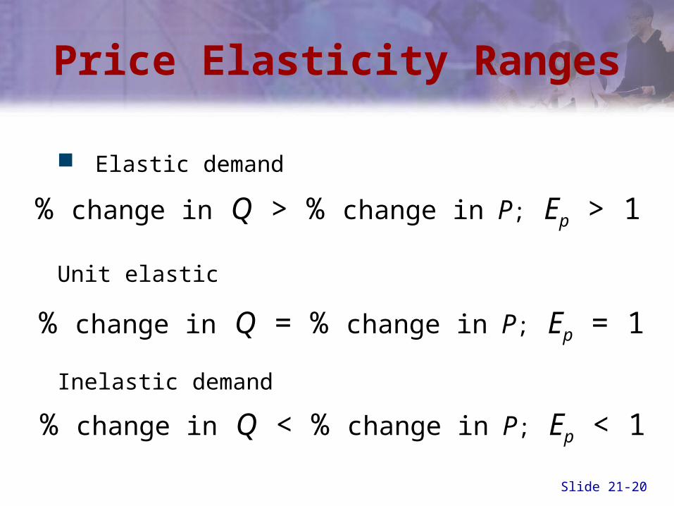
Elastic demand
Unit elastic
Inelastic demand
% change in Q > % change in P; Ep > 1
% change in Q = % change in P; Ep = 1
% change in Q < % change in P; Ep < 1
Slide 21-21
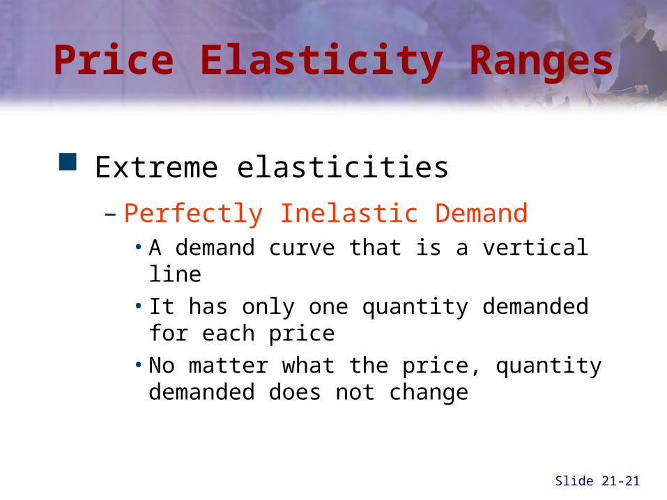
Price Elasticity Ranges
Extreme elasticities
– Perfectly Inelastic Demand• A demand curve that is a vertical line• It has only one quantity demanded for each
price• No matter what the price, quantity demanded
does not change

Slide 21-22
Extreme Price Elasticities
Quantity Demanded per Year(millions of units)
Pric
eD
Perfect inelasticity, or zero elasticity
80
Figure 21-1, Panel (a)

Slide 21-23
Extreme Price Elasticities
Quantity Demanded per Year(millions of units)
Pric
eD
80
P0
P1
Perfect inelasticity, or zero elasticity
Figure 21-1, Panel (a)

Slide 21-24
Price Elasticity Ranges
Extreme elasticities
– Perfectly Elastic Demand• A demand curve that is a horizontal line• It has only one price for every quantity• The slightest increase in price leads to zero
quantity demanded

Slide 21-25
Extreme Price Elasticities
Quantity Demanded per Year(millions of units)
Pric
e (c
ents
)
30
0
Perfect elasticity, or infinite elasticity
D
Figure 21-1, Panel (b)

Slide 21-26
Policy Example:Who Pays Gasoline Taxes?
State and federal governments impose gasoline taxes that are assessed as a flat amount per gallon.
Who pays the tax depends on price elasticity of demand.

Slide 21-27
Policy Example: Who Pays Gasoline Taxes?
Figure 21-2, Panels (a) and (b)

Slide 21-28
Policy Example: Who Pays Gasoline Taxes?
Figure 21-2, Panel (c)

Slide 21-29
Elasticity and Total Revenues
When demand is elastic, a negative relationship exists between small changes in price and changes in total revenue.
When demand is unit-elastic, changes in price do not change total revenue.
When demand is inelastic, a positive relationship exists between changes in price and total revenues.

Slide 21-30
Determinants of Price Elasticity of Demand
Existence of substitutes– The closer the substitutes and the more
substitutes there are, the more elastic is demand.
Share of the budget– The greater the share of the consumer’s
total budget spent on a good, the greater is the price elasticity.

Slide 21-31
Determinants of Price Elasticity of Demand
The length of time allowed for adjustment
– The longer any price change persists, the greater is the price elasticity of demand.• Price elasticity is greater in the long-run than
in the short-run.

Slide 21-32
Determinants of Price Elasticity of Demand
How to define the short run and the long run
– The short run is a time period too short for consumers to fully adjust to a price change.
– The long run is a time period long enough for consumers to fully adjust to a change in price other things constant.

Slide 21-33
Short-Run and Long-RunPrice Elasticity of Demand
In the short run, quantitydemanded falls slightly.However, with more timefor adjustment the demand curve becomesmore elastic and quantitydemanded falls by a greater amount.
D1
Pe
Q2
E
D2
Q1 Qe
P1
Pric
e pe
r U
nit
Quantity Demanded per Period
Figure 21-4

Slide 21-34
Short-Run and Long-RunPrice Elasticity of Demand
In the short run, quantitydemanded falls slightly.However, with more timefor adjustment the demand curve becomesmore elastic and quantitydemanded falls by a greater amount.
D1
Pe
Q2
E
D2
Q1 Qe
P1
Q3
D3
Pric
e pe
r U
nit
Quantity Demanded per Period
Figure 21-4

Slide 21-35
Example: Real-WorldElasticities of Demand
Table 21-2

Slide 21-36
Cross PriceElasticity of Demand
Cross Price Elasticity of Demand (Exy)
– The percentage change in the demand for one good (holding its price constant) divided by the percentage change in the price of a related good
– The responsiveness of change in demand of one good to the change in prices of related goods

Slide 21-37
Cross PriceElasticity of Demand
Formula for computing cross elasticity of demand
% change in demand for good X
%change in price of good YExy =

Slide 21-38
Cross PriceElasticity of Demand
Substitutes
– Exy would be positive• An increase in the price of X would increase
the quantity of Y demanded at each price.
Complements
– Exy would be negative• An increase in the price of X would decrease
the quantity of Y demanded at each price.

Slide 21-39
E-Commerce Example:Cross-Price Elasticity of Telescopes
Economic researchers have estimated the cross-price elasticity of demand for different types of telescopes.
The finding was that the cross-price elasticity of demand between 3.5-inch and 5-inch telescopes was 13.33.
In contrast, the cross-price elasticity of demand between 5-inch and 8-inch telescopes was close to zero.

Slide 21-40
E-Commerce Example:Cross-Price Elasticity of Telescopes
The conclusion is that 3.5-inch telescopes and 5-inch telescopes are substitutes for one another. But consumer behavior shows that the 5-inch telescope is not a substitute for the 8-inch one.

Slide 21-41
Income Elasticity of Demand
Income Elasticity of Demand (Ei)
– The percentage change in demand for any good, holding its price constant, divided by the percentage change in income
– The responsiveness of demand to changes in income, holding the good’s relative price constant

Slide 21-42
Income Elasticity of Demand
percentage change in demand
percentage change in incomeEi =

Slide 21-43
Income Elasticity of Demand
Income elasticity of demand – refers to a horizontal shift in the demand
curve in response to changes in income
Price elasticity of demand – refers to a movement along the curve in
response to price changes

Slide 21-44
Income Elasticity of Demand
Formula:
Change in Quantity ÷ Change in IncomeAverage Quantity Average Income
The income elasticity of demand can be either negative or positive.
Remember that, in calculating the income elasticity of demand, the price of the good is assumed to be constant.

Slide 21-45
Elasticity of Supply
Price Elasticity of Supply (Ei)
– The responsiveness of the quantity supplied of a commodity to a change in its price
– The percentage change in quantity supplied divided by the percentage change in price

Slide 21-46
Elasticity of Supply
Formula for computing price elasticity of supply
percentage change in quantity supplied
percentage change in priceES =

Slide 21-47
Elasticity of Supply
Classifying supply elasticities
– Perfectly Elastic Supply • Quantity supplied falls to zero when there is
any decrease in price.• The supply curve is horizontal at a given price.

Slide 21-48
Elasticity of Supply
Classifying supply elasticities
– Perfectly Inelastic Supply• Quantity supplied is constant no matter what
happens to price.• The supply curve is vertical at a given price.

Slide 21-49
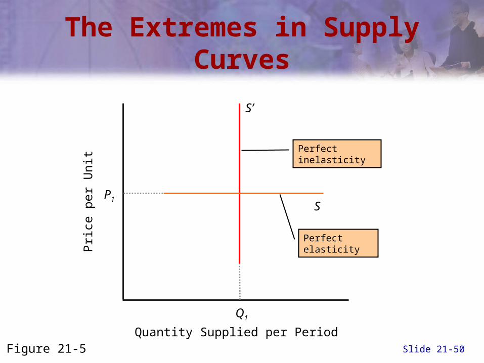
The Extremes in Supply Curves
Pric
e pe
r U
nit
Quantity Supplied per Period
Q1
S’
Perfect inelasticity
Figure 21-5
Slide 21-50
The Extremes in Supply Curves
Q1
Pric
e pe
r U
nit
Quantity Supplied per Period
P1S
S’
Perfect elasticity
Perfect inelasticity
Figure 21-5

Slide 21-51
Elasticity of Supply
Price elasticity of supply and length of time for adjustment
– The longer the time allowed for adjustment, the more elastic is supply.• Firms can find ways to increase (or decrease)
output.• Resources can flow into (or out of) an industry
through expansion (or contraction) of existing firms.

Slide 21-52
Short-Run and Long-Run Price Elasticity of Supply
Pe
Qe
Pric
e pe
r U
nit
Quantity Supplied per Period
S1
S2
As time passes the supply curve rotates from
S1 to S2 and quantity supplied rises first to Q1.
E
P1
Q1
Figure 21-6

Slide 21-53
Short-Run and Long-Run Price Elasticity of Supply
Pe
Qe
Pric
e pe
r U
nit
Quantity Supplied per Period
Q1
S1
S2
P1
As time passes the
supply curve rotates to S2 then to S3 and quantity supplied rises first to Q1 and then to Q2.
E
S3
Figure 21-6
Q2
Slide 21-54
Chinese competition caused the price of French truffles to fall 30 percent in 1996.
Accordingly French production decreased by 25%.
Short-run ES = .83
International Example: French Truffle Production Takes a Nosedive

Slide 21-55
Issues and Applications:The Inelastic Demand for Health Care
Evidence shows that the price elasticities of demand for physician services, hospital stays, and prescription medications are all 0.20 or less.
Yet the elasticity of demand for psychiatric services is about 1.20, six times greater than the price responsiveness for these other health care categories.

Slide 21-56
Issues and Applications:The Inelastic Demand for Health Care
The explanation is found in the fact that there are more substitutes available for psychiatric services.
Someone seeking help for emotional distress might consult a clergy member or a family counselor, rather than a psychiatrist.

Slide 21-57
Summary Discussion of Learning Objectives
Expressing and calculating the price elasticity of demand
– Percentage change in quantity demanded divided by the percentage change in price

Slide 21-58
Summary Discussion of Learning Objectives
The relationship between the price elasticity of demand and total revenues– When demand is elastic, price and total
revenue are inversely related
– When demand is inelastic, price and total revenue are positively related
– When demand is unit elastic, total revenue does not change when price changes

Slide 21-59
Summary Discussion of Learning Objectives
Factors that determine price elasticity of demand
– Availability of substitutes
– Percentage of a person’s budget spent on the good
– The length of time allowed for adjustment to a price change

Slide 21-60
Summary Discussion of Learning Objectives
The cross price elasticity of demand and using it to determine whether two goods are substitutes or complements– Percentage change in the demand for one good
divided by the percentage change in the price of another
– If cross elasticity is positive, the goods are substitutes
– If cross elasticity is negative, the goods are complements

Slide 21-61
Summary Discussion of Learning Objectives
Income elasticity of demand
– Percentage change in the demand for a good divided by the percentage in income

Slide 21-62
Summary Discussion of Learning Objectives
Classifying supply elasticities and how the length of time for adjustment affects price elasticity of supply– Elastic supply: price elasticity of supply is greater
than 1
– Inelastic supply: price elasticity of supply is less than 1
– Unit-elastic supply: price elasticity of supply is equal to 1
– The longer the time period for adjustment, the more elastic is supply

End of Chapter 21Demand and Supply Elasticity