Electronic copy available at: https://ssrn.com/abstract=2979391

Chapter 2: What Courts Do ... And How To Model It

Charles Cameron & Lewis Kornhauser∗

Princeton University and NYU School of Law

2 June 2017

Version 1.1

Abstract

We review the basic building blocks of the case-space approach to modeling courts,

particularly cases, dispositions, and rules. We provide numerous examples of case

spaces. We clarify the policy-making actions of courts, distinguishing statutory in-

terpretation, review of agency rule-making on procedural grounds, review of agency

rule-making on substantive grounds, and constitutionsl review. We demonstrate that

simple versions of the case-space approach are extensible to more complex legal con-

cepts such as evidence, doctrine, and causes of action. We note some of the feed

back effects of judicial actions, particularly on the distribution of presented cases, the

behavior in society at large, and on social welfare.

This essay is a draft chapter of a book-in-progress on the positive political theory

of courts.

Electronic copy available at: https://ssrn.com/abstract=2979391

I. Introduction

This chapter sets out a mathematical framework for modeling the actions of courts. We

use this framework throughout the book.

In our view, a satisfactory framework should satisfy five conditions. First and foremost,

the framework must capture the essential features of adjudication. Otherwise, one can hardly

be said to be modeling courts, as opposed to legislatures, bureaucracies, or chief executives.

Second, because courts interact with legislatures and the executive, the framework should

be able to express or accommodate these interactions. Put differently, we should be able

to embed models of courts within a constitutional order of separated powers. Third, the

framework should be extensible, flexible enough to investigate more complex features of ju-

dicial institutions and legal reasoning, such as doctrine and evidence. Fourth, the framework

should connect the operation of courts to the behavior of individuals and firms, as they

respond to judicial action. Put differently, we should be able to embed models of courts

within society. Finally, the framework should be straight-forward and tractable —easy to

learn and easy to use. We believe the framework laid out in this chapter satisfies those five

desiderata.

Because of its emphasis on cases, this framework is sometimes called the "case space

approach" to modeling courts. In fact, the case-space approach has applicability far beyond

courts. The same approach applies whenever an actor is presented with objects she must

process correctly according to rules, for example, when bureaucrats evaluate applications,

determine eligibilty for programs, or enforce regulations.1 It even applies when instructors

grade exams. The case space approach also can incorporate policy-making that occurs during

case processing.

The chapter is organized the following way. First, we review the basics of what courts

do. We then introduce the case-space approach to modeling judicial actions. We note some

possible extensions of the core components of the case-space approach. Finally, we suggest

some of the social implications of judicial actions, including feedback effects from judicial

1

Electronic copy available at: https://ssrn.com/abstract=2979391

actions to social consequences and the distribution of presented cases.

II. What Do Courts Do?

A court is a public body for resolving disputes in accordance with law. In

every case the court must determine what the facts are and what their legal

significance is. If the court determines their legal significance by applying an

existing rule of law unchanged, it is engaged in pure dispute resolution. But if to

resolve the dispute the court must create a new rule or modify an old one, that

is law creation. (Posner 1985:3, emphasis added)

This quotation, from a prominent federal judge and leading legal scholar, identifies the

distinctive features of a common law court. Hence, it identifies the basic concepts that a

formal framework of adjudication must accommodate: disputes, cases, facts, rules, dispute

resolution, and law creation. Let’s unpack Posner’s dense description, taking each piece in

turn.

First, a court is, in a certain sense, passive. Before a court can act, a litigant must ask

the court to act. Once asked, a court may be obliged to respond, at least if the petitioner

has standing (legally sanctioned access to the court) and follows designated procedures, and

the court has jurisdiction (legally sanctioned authority over the petitoner’s case). On the

other hand some courts, like the U.S. Supreme Court, have an almost entirely discretionary

docket, so they may choose freely from among the cases brought to them. Second, the

selected litigants present a case; i.e., a concrete, fact-ridden dispute between two or perhaps

more parties. Cases are central to all courts, not just common law courts. In civil law systems

even the highest appellate courts are case driven, though technically they decide only the

question of law raised by the case.2 Third, the Court must resolve this concrete dispute: it

determines which party prevails. Dispute resolution is not optional; it is obligatory in every

instance. So, the court cannot hold “don’t know” or “it’s a tie.” It is this disposition of

the case that “resolves”the dispute and thus is a necessary feature of adjudication. Fourth,

2

the court must resolve the dispute by applying law in the form of a rule to the facts in the

case. It is this feature of courts that make them principled rather than lawless. Indeed,

rule-driven dispute resolution is central to the very concept of rule of law. Finally, some

courts, particularly high appellate courts like the Supreme Court, may go beyond the simple

disposition of the case and make “policy” of a kind. We shortly return to exactly what

kind of policy these courts make. This policy-making action is what Posner means by "law

creation."

Modeling the actions of courts requires, minimally, a mathematical vocabulary that

instantiates the concepts of cases, facts, rules, and dispositions. As we discuss in the Bibli-

ographic Note for this chapter, judicial theorists developed this vocabulary during the early

and mid-1990s. It is increasingly used to model courts of all kinds both theoretically and

empirically. Because this mathematical vocabulary takes cases seriously, it is sometimes

called the "case space" approach to modeling courts.

Scholars trained in legislative studies or voting theory often feel some mental strain

upon encountering models that take judicial activities seriously. After all, when modeling

congressional voting or voting in referenda, one need only represent policies; there are no

cases and no case dispositions. As a result, legislative or electoral scholars frequently ask, If

I am just interested in policy, do I really need to bother with cases and case dispositions?

The answer is a resounding, “It depends.” More specifically, it depends on whether

dispositions interact with policy-making. If they do not, then dispositions may be ignored,

at least conceptually. For example, consider judicial review of an administrative regulation on

purely procedural grounds. Here, if the court rules that the agency obeyed the procedures

specified in the Administrative Procedures Act, it accepts the regulation. But if it rules

the Agency violated those procedures, it strikes down the regulation, effectively vetoing it.

In this decisional mode, the distinction between the case disposition (government prevails

vs. challenger prevails) and the policy action (acceptance of the regulation vs. veto of

the regulation) is slight. On the other hand, if dispositions and policy-making do interact,

3

then a formal model restricted to policy is apt to be misleading. An important example is

contemporary models of intra-court bargaining, discussed in Chapter 9. In many of these

models, case dispositions and policy-making interact profoundly —members of the Court

in the minority dispositional coalition do not participate in the bargaining over the policy

content of the majority opinion. If this is correct, one cannot get very far in understanding

policy-making on multi-member courts without incorporating dispositions. In Chapter 11,

we consider a model of statutory interpretation in which the Court modifies a legislative rule

only when confronted with particular cases, since often the Court can dispose of the case as

it wishes without modifying Congress’s rule. Here again, policy-making interacts profoundly

with cases and dispositions. Cases and case dispositions also play an essential role in the

models of judicial whistle-blowing and auditing in judicial hierachies, presented in Chapter

7. Examples may be found in most chapters of this book! Finally, most empirical studies of

courts rely on data about judicial case dispositions (which are abundant), not data about

judicial policies (which are diffi cult to devise). If the empirical work is to be grounded in

theory, the theory needs to incorporate the entity actually employed in the empirics. In sum,

treating a court like a cut-down legislature is intellectually unsatisfying; more than that, it

is likely to be misleading. Fortunately, taking cases seriously isn’t terribly diffi cult.

Suppose one wants to take cases seriously. Doing so places at least two demands on

the analyst. First, the model must be able to represent cases. Thus, the model must have

some space of cases. Second, the model must include the "rendering of judgment" among

the actions the judge takes.3 We shall typically call the rendered judgment a "disposition."

So the model must also include some space of possible dispositions. In addition, as noted by

Posner, courts sometimes create or modify rules; we turn to policy making shortly.

III. The Basics: Cases, Dispositions, and Rules

In the case-space approach to modeling courts, there is a space of possible cases, X,

with a specific case x ∈ X. A case connotes a legally relevant event that has occurred, e.g.,

4

the actual level of care exercised by a specific manufacturer, the degree of intrusiveness of a

particular police search, the speed of a given car on the highway. The space of cases is then

all possible legally relevant events, e.g., the possible levels of care, the possible degrees of

intrusiveness, or the possible speeds of the car. The case space X can be a high dimensional

space so that x is a vector (a point) in that space (we analyze an example in Appendix

A). Or, X could be the possible nodes in a lattice with x a particular node. Typically

though, we assume the set of possible cases may be represented by the real line (X = R),

hence x is a scalar. Through artful definition of the case space (e.g., intrusiveness of search,

entanglement of church and state, likelihood of harm to returned political asylum seeker,

degree of procedural regularity in the formulation of an agency rule), this simplification is

much more flexible than it might initially appear.

A case space is the basic building block of a model of adjudication. To go further

requires an understanding of what courts do. As Posner noted, courts resolve disputes. In

our framework, courts decide cases. Technically, a resolution has two elements: a disposition

and, should the plaintiffprevail, a remedy. The disposition of the case determines which party

prevails in the dispute between the litigants. The remedy may be an award of damages or

an injunction directing the plaintiff to take some action. These two resolutions correspond

to two distinct phases in a dispute resolution: a liability phase that determines who wins,

via the case disposition; and a remedial phase that determines the remedy.

We consider the disposition the nub of dispute resolution. Denote the set of outcomes

or dispositions as D = {0, 1}. A disposition is thus d, with 0 connoting a disposition in

favor of one litigant and 1 connoting a disposition in favor of the other. In what follows we

shall largely ignore the remedy.4 But, in some contexts, it may be reasonable to posit a set

of remedial outcomes —that we might denote R = R where R denotes the real line. This

approach allows fines, penalties, transfers, sentence lengths and the like.

A legal rule maps a case space into the outcome space. Thus, a judicial rule maps the set

of possible cases into possible dispositions, r : X → D. In words, it indicates the "correct"

5

disposition given the event that occurred. This is the nub of dispute resolution according to

law: given what occurred, who is entitled to win the dispute under law?5

Call the space of possible legal rules Rx. Notice that Rx is a set of functions from

X into D, and these functions may be very complex. However, we typically adopt a more

geometrical and restricted characterization. Given a one-dimensional case space, we restrict

the set of legal rules to the set of cut-point rules. A rule with a cut-point has the form:

(1) r(x; y) =

1 if x ≥ y

0 otherwise

where y denotes a cut-point. A universally familiar example is a speed limit. Here, a case is

the speed of a car. The case space X = R+, the non-negative real numbers, encompasses all

possible speeds of a car. The legal rule is a cut-point rule in which a driver is not speeding if

the speed of the car is below the speed limit y, while the driver is speeding if the speed of the

car is above the speed limit. Similarly in the case of tort law, in one formulation Defendant

is not liable if Defendant exercised at least as much care as the cutpoint y. Other examples

include allowable state restrictions on the provision of abortion services by medical providers;

state due process requirements for death sentences in capital crimes; the degree of procedural

irregularities allowable during elections; the required degree of compactness in state electoral

districts; the allowable extent of religious intrusion into government operations; the allowable

extent of gender-based distinction in employment; and the allowable degree of intrusiveness

of police searches. Many other examples of cutpoint rules may suggest themselves to the

reader. So, though cut-point rules are a significant simplification, they are more flexible than

one might initially suppose.

One small caveat is in order, though. Analysts typically index cut-point rules by the

value of the cut-point. This practice, though handy, can lead to a confusion of the case

space X (e.g., possible speeds of the car) and the space of rules or policies Rx (e.g., possible

speed limit rules). The examples in Appendix A highlight this point because in them, the

6

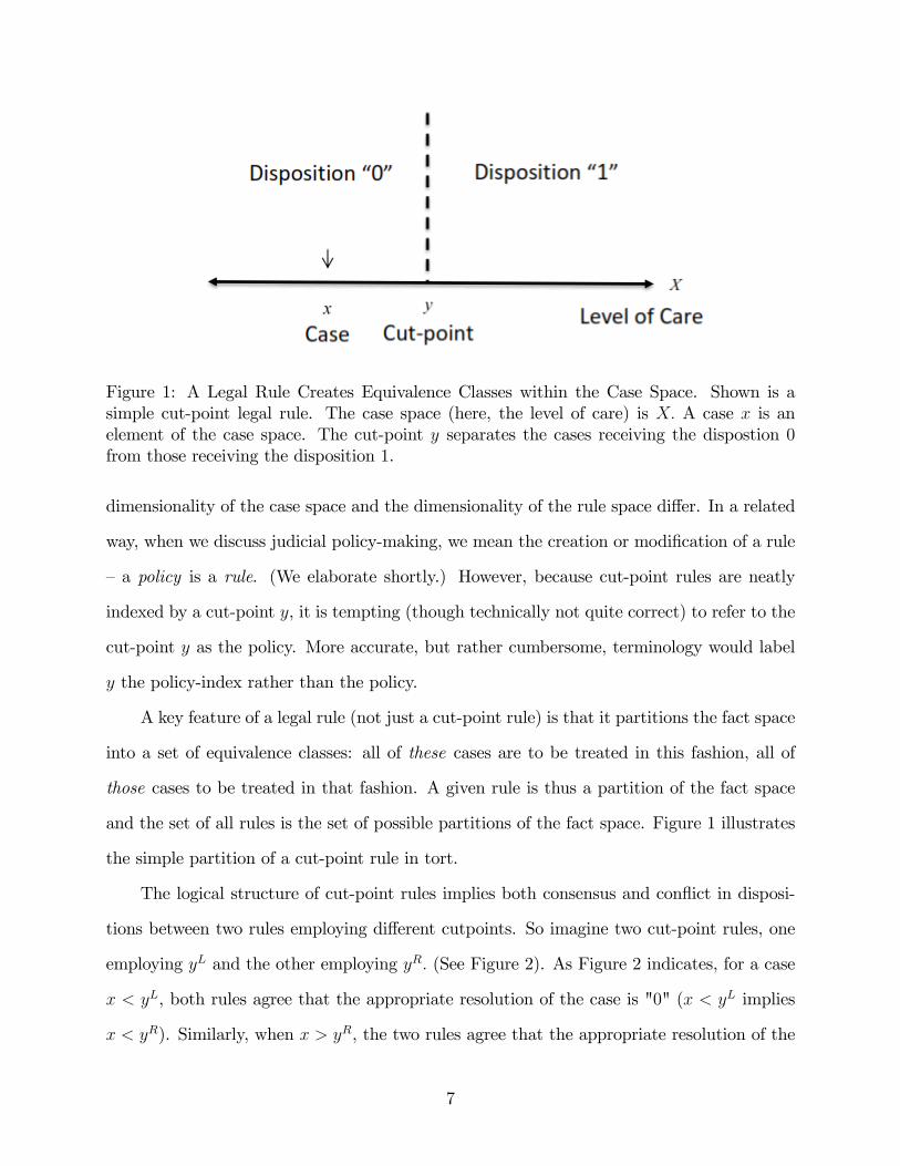
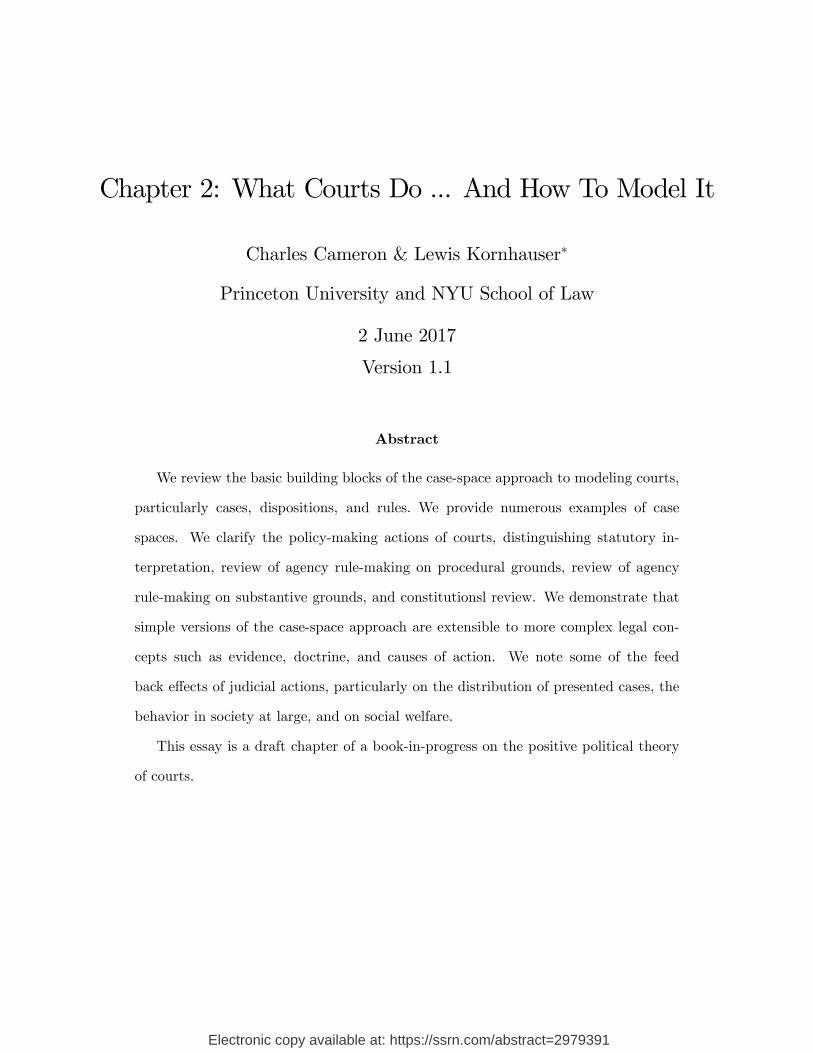
Figure 1: A Legal Rule Creates Equivalence Classes within the Case Space. Shown is asimple cut-point legal rule. The case space (here, the level of care) is X. A case x is anelement of the case space. The cut-point y separates the cases receiving the dispostion 0from those receiving the disposition 1.

dimensionality of the case space and the dimensionality of the rule space differ. In a related

way, when we discuss judicial policy-making, we mean the creation or modification of a rule

—a policy is a rule. (We elaborate shortly.) However, because cut-point rules are neatly

indexed by a cut-point y, it is tempting (though technically not quite correct) to refer to the

cut-point y as the policy. More accurate, but rather cumbersome, terminology would label

y the policy-index rather than the policy.

A key feature of a legal rule (not just a cut-point rule) is that it partitions the fact space

into a set of equivalence classes: all of these cases are to be treated in this fashion, all of

those cases to be treated in that fashion. A given rule is thus a partition of the fact space

and the set of all rules is the set of possible partitions of the fact space. Figure 1 illustrates

the simple partition of a cut-point rule in tort.

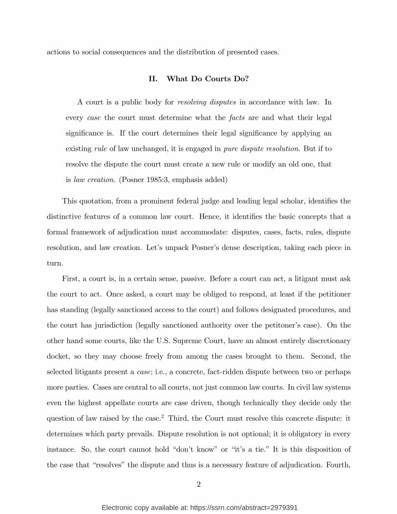
The logical structure of cut-point rules implies both consensus and conflict in disposi-

tions between two rules employing different cutpoints. So imagine two cut-point rules, one

employing yL and the other employing yR. (See Figure 2). As Figure 2 indicates, for a case

x < yL, both rules agree that the appropriate resolution of the case is "0" (x < yL implies

x < yR). Similarly, when x > yR, the two rules agree that the appropriate resolution of the

7

Figure 2: Conflict and Concensus Regions Induced by Two Distinct Rules. The structureof doctrine creates conflict and consensus regions when two judges disagree over the propercutpoint to enforce.

case is "1". Only when x ∈ [yL, yR] do the rules disagree: yL < x < yR implies that the L

doctrine holds the appropriate resolution of x is "1" while the R doctrine holds the appro-

priate resolution is "0". In many settings, we are interested in what happens in this conflict

region —the [yL, yR] interval where the two rules disagree about the correct disposition.6

A one dimensional case space with a cut-point rule provides a simple setting in which

to study adjudication. The one dimension-one parameter set-up is attractive because it

captures the essence of cases and rules, is extremely tractable, yet rich enough to build

interesting models of courts.

Most of the models in this book utilize this simple setting. But the case space formalism

is hardly restricted to such settings. Many extensions are straight forward. For instance, one

may increase the dimensionality of the case space to a more realistic size. Most legal rules

condition liability on many legal facts; the accident law example that motivates the cut-point

rule focuses on only one element, reasonable care, that the plaintiffmust establish to prevail.

The actual cause of action depends not only the "reasonable care fact" but also on facts about

causation, proximate causation, and harm. The case space is thus at least four-dimensional.

Empirical applications often must consider quite complex case spaces (see, e.g., Cameron et

8

Mode Actors Judicial Action Notation Status QuoStatutory H, S, P , J ; Disposition + d(x), yJ None once J moves becauseInterpretation or, J1-J9 Rule no actor has a veto over the ruleAdministrative A, J Disposition d(x) Judicial action restores aLaw —Procedure (judicial veto) prior ruleAdministrative A, J ; or Disposition + d(x), Judicial action restores aLaw —Substance H, S, P , A, J Block-veto y←−

J , −→y J prior rule but blocks some rules

Constitutional J , C; or Disposition + d(x), Judicial action restores aReview J, L; or J, P Block-veto y←−

J , −→y J prior rule but blocks some rules

Table 1: Decisional Modes of Judicial Policy-making. (See text for notation.)

al. 2000.). Similarly, one may enrich the space of possible rules, allowing complex partitions

of even simple case spaces. In general, though, we believe essential principles are clearest in

simple settings.

IV. Judicial Policy Making

As Posner noted, common law appellate courts often go beyond disposing of cases —

though they must always do that —to create policies. Policy-making is actually the primary

business of apex courts like the U.S. Supreme Court. What are these policies and how can

they be modeled?

Broadly speaking, courts like the U.S. Supreme Court engage in policy-making in three

distinct modes: 1) statutory interpretation; 2) administrative law, particularly the review

of agency rule-making but sometimes executive orders; and 3) constitutional review, partic-

ularly (for the U.S. Supreme Court) review of federal statutes, state statutes, or executive

actions. Policy-making actions in these venues are somewhat distinct from each other and

need to be modeled in somewhat different ways.

Table 1 provides information about appellate court decision-making in each decisional

mode, further distinguishing between review of administrative rules on procedural grounds

and their review on substantive grounds. In the table, the notation is as follows: H = House

of Representatives, S = Senate, P = President, A = Agency, C = Congress, J = Supreme

9

Court, L = state or local government, J i= Justice i, d(x) = disposition of case x, yJ =

judicially created cut-point, y←−J= floor on allowable cut-points, −→y J= ceiling on allowable

cut-points. The second column in the table indicates typical players in game theoretic

models of the decisional mode. For example, models of substantive review of agency rules

typically include players such as an Agency, the Court, but also the House, the Senate, and

the President. On the other hand, models of bargaining on a multi-member appellate court

focus on the judges themselves. The third column in Table 1 indicates the nature of the

court’s decision, e.g., a disposition plus the creation of a new rule or a disposition and the

veto of a proposed rule. The fourth column indicates the modeling convention associated

with the judicial action. Finally, the fifth column indicates the role of the status quo ante

in each mode, a somewhat vexed question.

A. Statutory Interpretation and Judicial Rule Making

Here is a definition of statutory interpretation: A court engages in statutory interpreta-

tion when it alters or modifies a policy or rule created by a legislature. This is a very broad

definition, which covers mild forms such as disambiguation of unclear statutory language, all

the way to deliberate substitution by the court of a new rule for the statutorily mandated

one.

In models of statutory interpretation, such as Ferejohn and Weingast 1992, Schwartz et

al 1994, or Iaryczower et al 2002 , the court creates a policy. In the formalism introduced

above, the court creates its own cut-point yJ for use in Equation 1, which it then applies to

the instant case to derive the disposition d(x). Presumably the court will use this rule to

dispose of future cases, unless Congress over-rules the court’s rule by enacting a new statute.

A subtlety, indicated in the last column of Table 1, is that under U.S. law Congress has no

mechanism simply to veto the court’s rule and thereby re-establish the original statutory rule

r(x; yC). Rather, Congress must enact a new statute articulating a new rule r′(x; yC). The

original statutory rule is thus irrelevant once the court acts. The court’s rule becomes the

10

effective status quo, much as the President’s unilateral action becomes the effective status

quo in models of unilateral executive action (see Moe and Howell 1999, Howell 2003).

B. Administrative Rule-making, Rule Vetoes, and Block-Vetoes

Courts review rules promulgated by administrative agencies. There are a variety of

grounds on which a court may do so. However, it is useful to distinguish procedural review

from substantive review. The former determines whether the administrative agency properly

followed the procedures specified in the Administrative Procedures Act. The latter typically

hinges on whether the agency’s interpretation of a statute was proper, that is, whether the

agency actually had legislative authority to formulate the rule that it issued. For example,

does the Environmental Protection Agency have the authority under the Clean Air Act to

regulate carbon emissions from power plants?

In terms of the formalism introduced above, procedural review is straight-forward. The

case space can be viewed as “extent of procedural regularity in rule-making,”the Agency’s

rule is a point in this space, and the cut-point in Equation 1 indicates an obligatory level of

procedural regularity. If the Agency’s rule-making failed to meet or exceed the obligatory

level of procedural regularity, the rule fails on procedural grounds. Thus the disposition

d(x) = 0 denotes a decision in favor of complainant and effectively vetoes the instant rule,

while the disposition d(x) = 1 denotes a decision in favor of the agency and effectively

accepts the instant rule, at least on procedural grounds. Arguably, there is no policy making

by the court at all, but simply enforcement of the Administrative Procedures Act. A judicial

veto of the instant regulation restores the status quo prior to the issuance of the Agency’s

regulation. A nearly equivalent formalization would have the Agency propose a policy, and

the Court veto or accept the policy (see for instance Ferejohn and Shipan 1990 or Gely and

Spiller 1990, discussed in Chapter 11).

Substantive review is a more complex matter. The Agency establishes a rule r(x, yA)

which it intends to use to regulate the conduct of some entities, e.g., firms, individuals,

11

or state or local governments. (The conduct of these entities becomes the cases x feeding

into the Agency’s rule.) The Agency justifies its rule via an interpretation of a statute,

such as the Clean Air Act or the Food and Drug Act. When the Court reviews the rule

on substantive grounds, it may review the Agency’s interpretation of the statute, not just

the agency’s rule-in-hand. Rejecting the Agency’s statutory interpretation naturally rejects

the Agency’s rule-in-hand —but it often implicitly or explicitly rejects many other possible

rules as well. And conversely, accepting the Agency’s statutory interpretation accepts the

Agency’s rule-in-hand but may implicitly accept a variety of other possible rules as well.

Using the formal notation, the action by the Court imposes restrictions on the set of

possible Agency rules, the set Rx. This restriction may be quite complex. But in the

simplified setting of one-dimensional cut-point rules like Equation 1, the Court’s actions

often take the form of a floor on allowable cut-points ( y←−J), or a ceiling on allowable cut-

points (−→y J). In the former case, any cut-point set by the Agency must exceed y←−J ; In the

latter, any cut-point established by the Agency may not exceed −→y J . In either case, the

Court vetoes not a single proposed rule but a block of possible rules, hence its action is a

block-veto. If the Court strikes down the Agency’s rule using a block-veto then, just as in a

rule-veto, its action re-establishes the status quo ante. Of course, Congress can legislatively

reverse the Court’s block-veto, by giving the Agency new statutory authority or by asserting

that the Agency’s understanding of its prior authority was correct.

C. Constitutional Review and Block-Vetoes

Supreme Court review of statutes or executive action on constitutional grounds strongly

resembles substantive review of agency rules, with the obvious difference that Congress

cannot legislatively reverse the Court’s ruling.

12

V. Beyond the Basics: Extensibility

Our exposition thus far has outlined the basic structure of case space. These are the

concepts and notation that will be used over and over in this book. However, the formalism

may be further elaborated to explore other features of adjudication, many of which are of

considerable interest to judicial scholars. In this section, we briefly discuss the distinction

between evidence and legal facts, and the concept of doctrine and related matters such as

legal issues and causes of action. Although the case-space framework can easily accommodate

these concepts, to date very little formal analysis has embraced them.

A. Evidence, Facts, and Rules

Disputes may arise for distinct types of reasons. In some cases, the parties might agree

about the norms of behavior but disagree about what happened. In a simple property

dispute, for example, adjoining landowners A and B may agree that A has no right to

construct a building within five feet of the boundary line marking their parcels but disagree

about where the boundary line is. Alternatively, the parties may agree about the facts, but

disagree about the norms that govern the conduct in dispute. Suppose, for example, that

B’s property fronts on the ocean and that, under state law, the beach up to the mean high

water mark is public. A and B may disagree whether state law grants A the right to cross

B’s property to reach the public beach.

In most disputes, both what happened —the facts —and the content of the prevailing

norms are in dispute. The literature on courts, however, has focused on this second, norma-

tive or policy aspect of disputes. This focus somewhat distorts not only the role of courts

but how courts apply and create legal rules.

As we discussed, a legal rule is a mapping from a set of legal facts to a disposition. At

trial, the finder of fact examines evidence and then draws the factual conclusions that permit

the application of the rule. Often the finder of fact has discretion about what facts to find

from a given body of evidence. Thus, two fact-finders considering the same evidence may

13

reach different conclusions of (legal) fact. This discrepancy may easily arise under standards

such as "reasonable care" or with respect to legal facts about mental states. We do not

observe mental states directly (if they exist at all) and hence on the same evidence one

fact finder might find that an agent acted "intentionally" while another fact finder would

conclude that she had acted recklessly. There is thus not a unique mapping from evidence

into legal facts, and hence no unique mapping from evidence into dispositions.7

We motivated our example of a cut-point rule by reference to a negligence rule in

which the cut-point constituted the standard of care that the agent must meet. This stylized

example has many uses but it surely does not fully capture the fact-finding process and the

relation between evidence and legal facts. "Reasonable care" is not a precise rule but a

standard; reasonable care refers to the care that a reasonable person would take under the

relevant conditions. In the driving example, reasonable care would depend not only on the

car’s speed but the amount of traffi c, the condition of the road, and the weather. As a result

one fact-finder might conclude that driving at 50 m.p.h. on a curving road when it is dark

and foggy is "reasonable care" and another fact-finder conclude the driver was negligent.

These considerations are real but lie, at present, at or beyond the research frontier. In

our opinion, civil procedure is a natural and logical venue for the case space approach. But

exactly how this field of endeavor will play out is a matter for the future.

B. Doctrine, Legal Issues, and Causes of Action

The definition of a legal rule as a mapping from a case space into the binary outcome

space D essentially treats a legal rule as a list: the rule matches a disposition to each case. In

some sense, to resolve the dispute, the court looks down the list until it finds the case before

it and then applies the disposition indicated on the list. In a one-dimensional case space with

a cut-point rule, reading this list is simple. When the case space has more dimensions, the

list may prove very complex with further complexity added by the tangled knots of evidence

the fact-finder must consider. A court thus has reason to search for a more perspicuous

14

way than a list to present the legal rule. A more comprehensible and accessible approach

facilitates a high court’s management of lower courts as well as making it easier for citizens

to comply with the rule.

A legal doctrine —or at least a good doctrine —states the rule in a more perspicuous

manner. It does so by decomposing the rule into a set of interrelated but simpler inquiries

that are typically called "issues." One may understand each issue as a lower dimensional

case space which we may call an issue space S and which we shall write C|s ; its resolution

depends on the partition of that issue space. An issue, that is, is a mapping from some

subset of case space C|s into the outcome space D. To resolve the case, the court must then

aggregate the resolutions of the issues. If, for example, there are four issues Ij, each defined

by an issue space C|s and a mapping fs : C|s → D, then the resolution of the case is defined

by a function fD : D4 → D. Typically, a doctrine is conjunctive; plaintiff wins only if she

prevails on each issue; i.e., fs(c) = 1 for each issue s. Put differently f(c) = mins fs(c). As

we discuss in Chapter 10, this structure of doctrine presents diffi culties on collegial courts

when the views of different judges are aggregated into a decision of the court.

Some doctrine is not conjunctive. Some rules direct the court to "balance" a set of legal

facts and these doctrines have a different structure. Proportionality tests in the constitutional

law of Canada, for example, has this balancing structure as does the rule of reason under

US antitrust law.

It is important to distinguish between a doctrine and doctrine. The latter might be

understood as the compendium of individual doctrines. Following Kornhauser 1992b we

might understand each doctrine as a cause of action. A litigation often consists of multiple

causes of action. When the court resolves the dispute, it determines whether plaintiffprevails

on each cause of action; she prevails in the litigation if she prevails on one cause of action.

The multiplicity of causes of action united in a single litigation identifies an equivocation

in our terminology. A "case" colloquially refers to the dispute as a whole; and the opinion

written in a case, colloquially understood, will address each cause of action. In our technical

15

sense, however, each cause of action is a distinct case as it relies on a distinct legal rule and

distinct set of facts.8

As an example consider contract law. A contract dispute typically arises when the

promisee complains that the promisor did not meet its obligations under the contract. To

prevail, plaintiff must establish a variety of legal facts. She must first show that, in fact, a

contract existed between promisee and promisor. To do so, several issues must be resolved

favorably to plaintiff: was there an offer? was there an acceptance? Did the promisee

provide consideration to the promisor? Plaintiff must then prove that the promisor did

not perform the contract. The promisor might raise various defenses that would excuse

performance —mistake, frustration, impossibility. Each of these issues refers to distinct legal

facts and requires attention to a subset of the evidence that the fact-finder will consider. This

decomposition of the case into distinct issues facilitates the presentation and evaluation of

evidence as well as the application of the legal rule to the found facts.9

We might represent a doctrine by a decision tree. In the contract case, at the first node

the fact finder must determine whether an offer was made or not. To do so, she refers to the

relevant evidence. If an offer was not made, the contract cause of action fails and defendant

prevails; a disposition of 0 results. If an offer was made, the fact finder proceeds to the

next node at which she must determine whether the offer was accepted. If the offer was

not accepted, a disposition of 0 is again required. If the offer was accepted, the fact finder

proceeds to the next node at which the question of consideration is addressed. This tree

structure illustrates the structure of the conjunctive rule. Inducing such decision trees from

a statistical analysis of cases is a current research frontier in empirical judicial studies, see

e.g., Kastellec 2016. Very little theory has yet been developed for this representation of case

spaces, rules, and doctrine.

16

SocialBehaviors

x, Xz(x), Z(x), Ez(x)

Casesx, X

f(x), F(x), E(x)

Dispositions, Rules,Cut­points

d(x), r(x,y), y,D(x) = {d(x1), … d(xn)}

(2)(1)

Figure 3: Judicial Actions and Social Consequences. Social behaviors generate cases. Inturn, cases generate judicial actions. Then, judicial actions affect social behaviors and cases.See text for further elaboration.

VI. Judicial Actions and Social Consequences

Judicial actions have consequences. So, let’s be explicit about some of those conse-

quences (we will return to this material in Chapter 3 when we discuss judicial preferences).

Figure 3 provides a schematic device for thinking about judicial actions and their con-

sequences. Consider the space of possible social behaviors or acts X, for instance, the speed

of cars on interstate highways, the care taken by manufacturers, the assembly of citizens to

protest government actions, and so on. There is a density of actual social behaviors z(x), a

distribution of social behaviors Z(x), and an expected social behavior Ez(x). The distribu-

tion of social behaviors or acts gives rise to a set of social costs and benefits (not indicated

in the figure) and hence social welfare. In addition, the distribution of social behaviors gives

rise to judicial cases. The mechanisms by which a particular social act becomes a particular

judicial case are many (indicated by arrow (1) in the figure). These include law enforcement

as well as individual decisions to initiate legal action and settle legal disputes. The actual

set of legal cases is necessarily a subset of actual social behaviors. So the set of possible

legal cases is again X with a given case x ∈ X. And, there is a density of cases f(x), a

distribution of cases F (x), and an expected case E(x). Cases in turn give rise to the judicial

actions noted in Table 1. The mechanisms by which cases afford judicial action —indicated

by arrow (2) in Figure 3 —are the games we analyze in this book. As noted in the figure,

17

judicial actions include case dispositions, rules, and the selection of cut-points, and also the

use of block-vetoes and the creation of floors and ceilings. A series of judicial actions create

sets of judicial acts, for instance, the set of case dispositions D(x).

Because people are forward-thinking, judicial actions feed back into social behaviors and

hence the cases presented to courts. So, if a judge creates a new rule or changes an old one,

this action may well alter the distribution of cases subsequently presented to the court. And

it may alter the distribution of bevhaviors in society. Thus, the density of cases presented

to the court should more properly be written f(x; y) or perhaps f(x;D(x)), and similarly

the density of social actions should more properly be written z(x; y) or perhaps z(x;D(x)).

The extent to which judges anticipate these changes or indeed strive to bring them about, is

a complex issue we discuss in the next chapter. But certainly a social analyst may consider

how the design and operation of a judiciary —as connoted by arrow (2) —affects the actions

of judges, which in turn affect the cases presented to courts and the behavior of individuals

and firms in society at large. And those behaviors in turn affect social welfare.

VII. Bibliographic Note

The case-space approach to modeling courts was first formalized in Kornhauser 1992a

and Kornhauser 1992b. It has since become a work horse in the applied modeling of courts,

though many analysts continue to force courts into a legislative Procrustean bed. Lax 2011

provides a useful review of recent work. The case space approach was initially deployed in

an applied model in political science in Cameron et al. 2000., a formal model of certiorari

and compliance in the judicial hierarchy with empirical tests. The origin of what we dub

a block-veto is an extremely creative paper, Spiller and Spitzer 1992. The small literature

on policy floors and ceilings, e.g., due to federal mandates applied to state governments,

is highly relevant to judicial action, see Cremer and Palfrey 2000. Kastellec 2016 explores

some implications of judicial block-vetoes. With respect to extensibility, a formal model of

civil procedure is Sobel 1989. But in general this is a very under-tilled field. The social

18

welfare properties of specific legal rules is perhaps the central theme of the field of law and

economics. However, not surprisingly, relatively fews analyses fully articulate the linkages

between judicial behavior, the distribution of legal cases (including the efforts of law enforce-

ment and calculations of potential litigants), the distribution of social behaviors, and social

welfare. Though by now somewhat dated, Cooter and Rubinfeld 1989 takes a refreshingly

broad view of factors involved in arrow (1) in Figure 3.

A Advanced Examples

The examples in the text involve one-dimensional case spaces with one-parameter cut-

point rules. But the case space approach easily extends beyond the one dimension-one

parameter configuration. The following examples illustrate straight-forward ways to ex-

tend the basic framework. First we consider a two-dimensional case space with a legal rule

characterized by one parameter. Then we consider a single-dimensional case space with a

rule characterized by two parameters. One may extend these examples to n−dimensional

case spaces with m−parameter rules. However, we tend to avoid these notationally heavy,

insight-light settings

A. A Two-Dimensional Case Space with a One-Parameter Set of Rules

Spiller and Spitzer 1992 suggest that some doctrines in constitutional law can be treated

as partitions of a two-dimensional case space —they point to parts of discrimination law and

parts of First Amendment law (freedom of speech law). In tort law, relative negligence

affords another example. So suppose the case space X has two dimensions. A given case

is now a vector (x1, x2) (here, subscripts denote dimensions). For concreteness, imagine the

case space as the unit square, so the space is X = [0, 1]× [0, 1].

This two-dimensional space can be partitioned in many different ways. A particularly

useful partition uses a cutting line, x2 = ax1 + b. This set of cut-line rules is the obvious

generalization of the cutpoint rules in a one-dimensional case space. In two dimensions, a

19

Figure 4: Two dimensional case space with a one parameter rule. The case space is theunit square. The dark line (x2 = x1) represents the most-preferred rule of the judge. Analternative rule is x2 = max{x1 − b, 0}. The conflict zone is the space between the twocutting lines. In the figure, b = 1

4.

cut-line rule partitions the case space into two sets: Cases "above" the line receive one

disposition; cases "below" the other. So the enforced rule is:

r(x1, x2; a, b) =

1 if x2 ≥ ax1 + b

0 otherwise

We normalize the judge’s most-preferred partition as x2 = x1, the 45-degree line running

from the lower-left corner to the upper-right corner. In other words, the judge’s most-

preferred rule is r(x1, x2; a = 1, b = 0). We assume all other doctrines simply alter the

intercept b while retaining the slope parameter a = 1. This reduces the characterization of

cutting lines to the single parameter, b.

The case space and two cutting lines are shown in Figure 4.

20

Speed of Car

Disposition“0”Disposition “1”

Disposition“0”

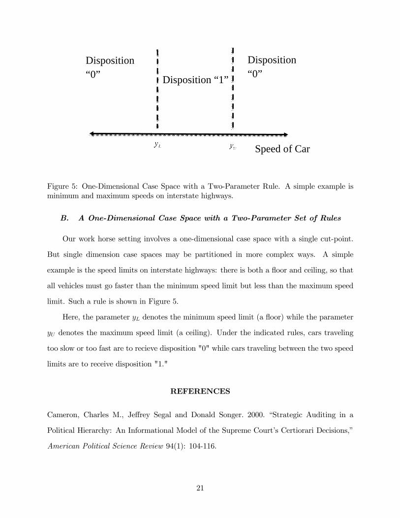
Figure 5: One-Dimensional Case Space with a Two-Parameter Rule. A simple example isminimum and maximum speeds on interstate highways.

B. A One-Dimensional Case Space with a Two-Parameter Set of Rules

Our work horse setting involves a one-dimensional case space with a single cut-point.

But single dimension case spaces may be partitioned in more complex ways. A simple

example is the speed limits on interstate highways: there is both a floor and ceiling, so that

all vehicles must go faster than the minimum speed limit but less than the maximum speed

limit. Such a rule is shown in Figure 5.

Here, the parameter yL denotes the minimum speed limit (a floor) while the parameter

yU denotes the maximum speed limit (a ceiling). Under the indicated rules, cars traveling

too slow or too fast are to recieve disposition "0" while cars traveling between the two speed

limits are to receive disposition "1."

REFERENCES

Cameron, Charles M., Jeffrey Segal and Donald Songer. 2000. “Strategic Auditing in a

Political Hierarchy: An Informational Model of the Supreme Court’s Certiorari Decisions,”

American Political Science Review 94(1): 104-116.

21

Cooter, Robert D. and Daniel L. Rubinfeld. 1989. "Economic Analysis of Legal Disputes,"

Journal of Economic Literature 27(3):1067-1097.

Cremer, Jacques, and Thomas R. Palfrey. 2000. "Federal Mandates by Popular Demand."

Journal of Political Economy 108(5): 905-927.

Ferejohn, John, and Charles Shipan. 1990. "Congressional Influence on Bureaucracy." Jour-

nal of Law, Economics, & Organization 6: 1-20.

Ferejohn, John and Barry Weingast. 1992. "A Positive Theory of Statutory Interpretation,"

International Review of Law and Economics 12:263-279.

Gely, Rafael, and Pablo T. Spiller. 1990. "A Rational Choice Theory of Supreme Court

Statutory Decisions with Applications to the ’State Farm’and ’Grove City’Cases." Journal

of Law, Economics, & Organization 6(2): 263-300.

Howell, William. 2003. Power Without Persuasion: The Politics of Direct Presidential Ac-

tion. Princeton University Press.

Iaryczower, Matías, Pablo T. Spiller, and Mariano Tommasi. 2002. "Judicial Independence

in Unstable Environments, Argentina 1935-1998." American Journal of Political Science :

699-716.

Kastellec, John. 2016. "Empirically Evaluating the Counter-Majoritarian Diffi culty: Public

Opinion, State Policy, and Judicial Review Before Roe v. Wade." Working paper, Depart-

ment of Politics, Princeton University.

Kornhauser, Lewis. 1992 a. "Modeling Collegial Courts I: Path Dependence," International

Review of Law & Economics, 12: 169-185.

Kornhauser, Lewis. 1992 b. "Modeling Collegial Courts. II. Legal Doctrine," Journal of Law,

Economics & Organization 8: 441-470.

22

Lax, Jeffrey. 2011. "The New Judicial Politics of Legal Doctrine," Annual Review of Political

Science 14:131-157.

Moe, Terry M., and William G. Howell. 1999. "The Presidential Power of Unilateral Action."

Journal of Law, Economics, and Organization 15.1 (1999): 132-179.

Posner, Richard. 1985. The Federal Courts: Crisis and Reform. Harvard University Press.

Schwartz, Edward P., Pablo T. Spiller, and Santiago Urbiztondo. 1994. "A Positive Theory

of Legislative Intent." Law and Contemporary Problems 57(1): 51-74.

Sobel, Joel. 1989. "An Analysis of Discovery Rules." Law and Contemporary Problems 52.1:

133-159.

Spiller, Pablo T. and Matthew L. Spitzer. 1992. "Judicial Choice of Legal Doctrines,"Journal

of Law, Economics, & Organization 8(1): 8-46.

23

Notes

∗For helpful comments we thank Sephir Shahshahani and Ben Johnson.

1The analysis of legislation might also benefit from a case space approach. As we define

below, a rule is simply a partition of case space; statutes are rules and they provide complex

partitions of case space. The Internal Revenue Code, for example, partitions a very complex

case space into equivalence classes defined by the amount of tax owed.

2Both intermediate and supreme appellate courts in common law systems also decide

only questions of law while in civil law systems intermediate appellate courts often have the

power to find facts as well. International courts similarly address concrete disputes.

Some constitutional courts, however, do not always decide cases. The french Conseil

Constitutionelle, for example, initially had only the power to decide the constitutionality of

bills referred to it by the Pariliament. These references did not entail the review of concrete

dispute.

3This approach thus excludes certain constitutional "courts" from consideration or some

actions of constitutional "courts" from consideration. The French Conseil Constitutionnel

is called a "council" not a "court" for a reason. At its origin, it had only authority for ex

ante review of statutes; it thus did not decide cases.

4Typically, the choice of remedy is delegated to the finder of fact and hence gives rise to

no legal issue on appeal other than whether the fact finder exceeded its discretion. This

question is dichotomous and fits within the doctrinal framework developed below

5It is worth noting that legislatures do something very different from courts. When a

legislature enacts a statute it defines a case space and a mapping into some outcome space

that need not be D. For instance, statutes define a case space and then a map into an

outcome space often R. The internal Revenue Code, for example, maps a complex fact

space into an amount of tax owed (which might be negative). The restriction to the outcome

space D is thus another characteristic feature of adjudication.

6The regions of conflict and consensus are a feature of general rules as well. Consider

24

two rules R and S each of which partitions the case space X. Let 1J be the set of points in

X, that rule J assigns the value 1 and 0J the set of points in X that rule J assigns the value

0. Then the region of consenus is simply (1R ∩ 1S) ∪ (0R ∩ 0S) while the conflict region is

simply (1R ∩ 0S) ∪ (0R ∩ 1S)7The fact finder does not have unlimited discretion. A court may hold that on given

evidence E no reasonable person could have concluded that defendant was negligent (or in

the alternative not negligent). But within the bounds developed by the court the fact finder

is unconstrained.

8Opinions in actual (colloquiual) cases present even more complex situations than the

text suggests. Often an opinion resolves multiple disputes. Two criminal defendants may

have been tried together. When each appeals a conviction, the appeals may be joined in

a single "case." But the facts relevant to each defendant differ; the opinion thus renders

judgment in two distinct cases in the technical sense of case space.

Similarly, a single dispute between the same parties may involve multiple instances of

the same cause of action. Consider, for example, Thornburgh v. Gingles, 478 US 30 (1986),

in which black citizens of North Carolina challenged the state’s redistricting plan. More

precisely, the plaintiffs contended that seven districts —House Districts 8, 21, 23, 36 and

39 and Senate Districts 2 and 22 —violated section 2 of the Voting Rights Act of 1965 as

amended. The dispute thus consisted of 7 identical causes of action. The District Court

agreed with plaintiffs and rejected the borders of all seven districts. The Attorney General

of North Carolina appealed the District Court decision with respect to five of the seven

voting districts. The Supreme Court, in a set of long, complex and contested opinions,

affi rmed in part and reversed in part. That is, it affi rmed the District Court’s judgment

that four of the five districts at the center of the appeal violated section 2 but reversed

with respect to House District 23. Each of the five districts constituted a distinct incident

(or case) as each represented a distinct concatenation of legally relevant facts under the

statute as interpreted by the Supreme Court of the United States. Indeed, the case yielded

25

two distinct dispostional majorities: For House District 23, the dispostional vote was 6-

3 (Justices Brennan, White, O’Connor, Burger, Powell and Rehnquist in the majority),

whereas the dispositional majority was unanimous for the other six voting districts. Thus

the statement "affi rmed in part, reversed in part" refers to the outcomes in the distinct

incidents; for each incident the outcome space is dichotomous.

9Doctrine like this might have two distinct forms. The issues might ground the cause

of action. Some scholars, for example, understand contract as grounded in the morality of

promise. The legal issues thus correspond to moral concerns that promise address.

Alternatively, doctrine may simply be a heuristic that presents the legal rule in a manner

that is more easily understood than a list.

26