1

CHAPTER 2

UPSIDE, DOWNSIDE: UNDERSTANDING RISKRisk is part of investing and understanding what it is and how it is measured

is essential to developing an investment philosophy. In this chapter, we will lay thefoundations for analyzing risk in investments. We present alternative models for measuringrisk and converting these risk measures into an expected return. We will also consider waysin an investor can measure his or her risk aversion.We begin with a discussion of risk and present our analysis in three steps. In the first step,we define risk in terms of uncertainty about future returns. The greater this uncertainty, themore risky an investment is perceived to be. The next step, which we believe is the centralone, is to decompose this risk into risk that can be diversified away by investors and riskthat cannot. In the third step, we look at how different risk and return models in financeattempt to measure this non-diversifiable risk. We compare and contrast the most widelyused model, the capital asset pricing model, with other models, and explain how and whythey diverge in their measures of risk and the implications for the equity risk premium. Inthe second part of this chapter, we consider default risk and how it is measured by ratingsagencies. In addition, we discuss the determinants of the default spread and why it mightchange over time.

What is risk?Risk, for most of us, refers to the likelihood that in life’s games of chance, we will

receive an outcome that we will not like. For instance, the risk of driving a car too fast isgetting a speeding ticket, or worse still, getting into an accident. Webster’s dictionary, infact, defines risk as “exposing to danger or hazard”. Thus, risk is perceived almost entirelyin negative terms.

In finance, our definition of risk is both different and broader. Risk, as we see it,refers to the likelihood that we will receive a return on an investment that is different fromthe return we expected to make. Thus, risk includes not only the bad outcomes, i.e, returnsthat are lower than expected, but also good outcomes, i.e., returns that are higher thanexpected. In fact, we can refer to the former as downside risk and the latter is upside risk;but we consider both when measuring risk. In fact, the spirit of our definition of risk infinance is captured best by the Chinese symbols for risk, which are reproduced below:

2

The first symbol is the symbol for “danger”, while the second is the symbol for“opportunity”, making risk a mix of danger and opportunity. It illustrates very clearly thetradeoff that every investor and business has to make – between the higher rewards thatcome with the opportunity and the higher risk that has to be borne as a consequence of thedanger.

Much of this chapter can be viewed as an attempt to come up with a model that bestmeasures the “danger” in any investment and then attempts to convert this into the“opportunity” that we would need to compensate for the danger. In financial terms, weterm the danger to be “risk” and the opportunity to be “expected return”.

Equity Risk and Expected ReturnTo demonstrate how risk is viewed in finance, we will present risk analysis in three

steps. First, we will define risk . Second, we will differentiate between risk that is specific toone or a few investments and risk that affects a much wider cross section of investments.We will argue that in a market where investors are well diversified, it is only the latter risk,called market risk that will be rewarded. Third, we will look at alternative models formeasuring this market risk and the expected returns that go with it.

I. Defining RiskInvestors who buy assets expect to earn returns over the time horizon that they hold

the asset. Their actual returns over this holding period may be very different from theexpected returns and it is this difference between actual and expected returns that is sourceof risk. For example, assume that you are an investor with a 1-year time horizon buying a 1-year Treasury bill (or any other default-free one-year bond) with a 5% expected return. Atthe end of the 1-year holding period, the actual return on this investment will be 5%, whichis equal to the expected return. The return distribution for this investment is shown inFigure 2.1.

3

Returns

Probability = 1

Expected Return

Figure 2.1: Probability Distribution for Riskfree Investment

The actual return is always equal to the expected return.

This is a riskless investment.To provide a contrast to the riskless investment, consider an investor who buys stock

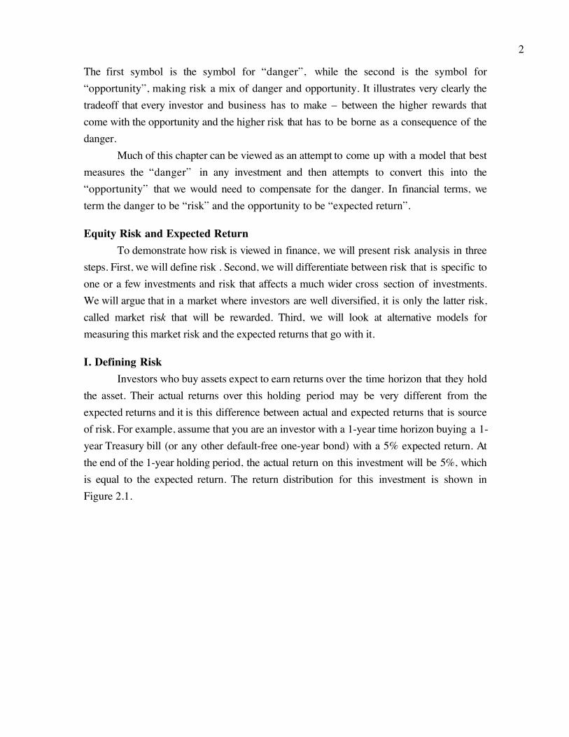
in a company like Cisco. This investor, having done her research, may conclude that she canmake an expected return of 30% on Cisco over her 1-year holding period. The actual returnover this period will almost certainly not be equal to 30%; it might be much greater or muchlower. The distribution of returns on this investment is illustrated in Figure 2.2.

4

ReturnsExpected Return

Figure 2.2: Probability Distribution for Risky Investment

This distribution measures the probabilitythat the actual return will be different fromthe expected return.

In addition to the expected return, an investor has to note that the actual returns, in this case,are different from the expected return. The spread of the actual returns around the expectedreturn is measured by the variance or standard deviation of the distribution; the greater thedeviation of the actual returns from expected returns, the greater the variance.

One of the limitations of variance is that it considers all variation from the expectedreturn to be risk. Thus, the potential that you will earn a60% return on Cisco (30% more than the expected return of30%) affects the variance exactly as much as the potentialthat you will earn 0% (30% less than the expected return).In other words, you do not distinguish between downsideand upside risk. This is justified by arguing that risk issymmetric – upside risk must inevitably create the potentialfor downside risk.1 If you are bothered by this assumption,you could compute a modified version of the variance, calledthe semi-variance, where you consider only the returns that fall below the expected return.

It is true that measuring risk with variance or semi-variance can provide too limited aview of risk, and there are some investors who use simpler stand-ins (proxies) for risk. Forinstance, you may consider stocks in some sectors (such as technology) to be riskier than

1 In statistical terms, this is the equivalent of assuming that the distribution of returns is close to normal.

The Most and LeastVolatile Stocks: Take a lookat the 50 most and 50 leastvolatile stocks traded in theUnited States, based upon 5years of weekly data.

5

stocks in other sectors (say, food processing). Others prefer ranking or categorizationsystems, where you put firms into risk classes, rather than trying to measure its risk in units.Thus, Value Line ranks firms into five classes, based upon risk.

There is one final point that needs to be made about how variances and semi-variances are estimated for most stocks. Analysts usually look at the past – stock prices overthe last 2 or 5 years- to make these estimates. This may be appropriate for firms that havenot changed their fundamental characteristics – business or leverage – over the period. Forfirms that have changed significantly over time, variances from the past may provide a verymisleading view of betas in the future.

II. Diversifiable and Non-diversifiable RiskAlthough there are many reasons that actual returns may differ from expected

returns, we can group the reasons into two categories: firm-specific and market-wide. Therisks that arise from firm-specific actions affect one or a few investments, while the riskarising from market-wide reasons affect many or all investments. This distinction is criticalto the way we assess risk in finance.

The Components of RiskWhen an investor buys stock or takes an equity position in a firm, he or she is

exposed to many risks. Some risk may affect only one or a few firms and it is this risk thatwe categorize as firm-specific risk. Within this category, we would consider a wide range ofrisks, starting with the risk that a firm may have misjudged the demand for a product fromits customers; we call this project risk. For instance, consider an investment by Boeing in anew larger capacity airplane that we will call the Super Jumbo. This investment is based onthe assumption that airlines want a larger airplane and will be willing to pay a higher pricefor it. If Boeing has misjudged this demand, it will clearly have an impact on Boeing’searnings and value, but it should not have a significant effect on other firms in the market.The risk could also arise from competitors proving to be stronger or weaker thananticipated; we call this competitive risk. For instance, assume that Boeing and Airbus arecompeting for an order from Qantas, the Australian airline. The possibility that Airbus maywin the bid is a potential source of risk to Boeing and perhaps a few of its suppliers. Butagain, only a handful of firms in the market will be affected by it. Similarly, the HomeDepot recently launched an online store to sell its home improvement products. Whether itsucceeds or not is clearly important to the Home Depot and its competitors, but it is unlikelyto have an impact on the rest of the market. In fact, we would extend our risk measures toinclude risks that may affect an entire sector but are restricted to that sector; we call this

6

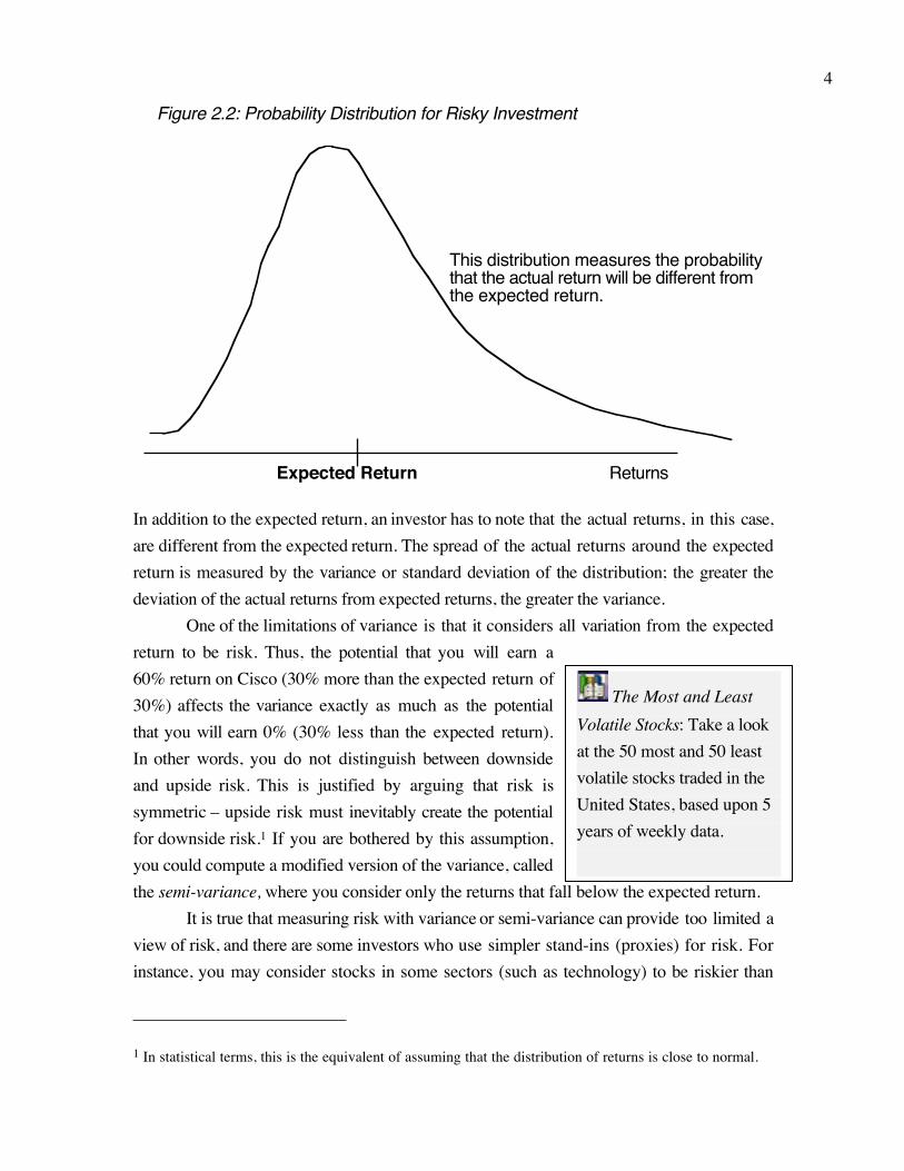
sector risk. For instance, a cut in the defense budget in the United States will adverselyaffect all firms in the defense business, including Boeing, but there should be no significantimpact on other sectors, such as food and apparel. What is common across the three risksdescribed above – project, competitive and sector risk – is that they affect only a small sub-set of firms.

There is other risk that is much more pervasive and affects many if not allinvestments. For instance, when interest rates increase, all investments are negativelyaffected, albeit to different degrees. Similarly, when the economy weakens, all firms feel theeffects, though cyclical firms (such as automobiles, steel and housing) may feel it more. Weterm this risk market risk.

Finally, there are risks that fall in a gray area, depending upon how many assets theyaffect. For instance, when the dollar strengthens against other currencies, it has a significantimpact on the earnings and values of firms with international operations. If most firms in themarket have significant international operations, it could well be categorized as market risk.If only a few do, it would be closer to firm-specific risk. Figure 2.3 summarizes the breakdown or the spectrum of firm specific and market risks.

Actions/Risk that affect only one firm

Actions/Risk that affect all investments

Firm-specific Market

Projects maydo better orworse thanexpected

Competitionmay be strongeror weaker thananticipated

Entire Sectormay be affectedby action

Exchange rateand Politicalrisk

Interest rate,Inflation & News about Econoomy

Figure 2.3: A Break Down of Risk

Affects fewfirms

Affects manyfirms

Why Diversification reduces or eliminates Firm-specific Risk: An Intuitive Explanation As an investor, you could invest your entire portfolio in one stock, say Boeing. If

you do so, you are exposed to both firm specific and market risk. If, however, you expandyour portfolio to include other assets or stocks, you are diversifying, and by doing so, youcan reduce your exposure to firm-specific risk. There are two reasons why diversificationreduces or, at the limit, eliminates firm specific risk. The first is that each investment in a

7

Highest R-squaredcompanies: Take a lookat the 50 companies withthe highest proportion ofmarket risk using the last5 years or weekly data.

diversified portfolio is a much smaller percentage of that portfolio than would be the case ifyou were not diversified. Thus, any action that increases or decreases the value of only thatinvestment or a small group of investments will have only a small impact on your overallportfolio, whereas undiversified investors are much more exposed to changes in the valuesof the investments in their portfolios. The second reason is that the effects of firm-specificactions on the prices of individual assets in a portfolio can be either positive or negative foreach asset in any period. Thus, in very large portfolios, this risk will average out to zero andwill not affect the overall value of the portfolio.

In contrast, the effects of market-wide movements are likely to be in the samedirection for most or all investments in a portfolio, thoughsome assets may be affected more than others. For instance,other things being equal, an increase in interest rates willlower the values of most assets in a portfolio. Being morediversified does not eliminate this risk.

One of the simplest ways of measuring how muchrisk in a firm is firm specific is to look at the proportion ofthe firm’s price movements that are explained by themarket. This is called the R-squared and it should rangebetween zero and one can be stated as a percentage; it measures the proportion of the firm’srisk that comes from the market. A firm with an R-squared of zero has 100% firm specificrisk whereas a firm with an R-squared of 0% has no firm specific risk.

Why is the marginal investor assumed to be diversified?The argument that diversification reduces an investor’s exposure to risk is clear both

intuitively and statistically, but risk and return models in finance go further. The modelslook at risk through the eyes of the investor most likely to be trading on the investment atany point in time, i.e. the marginal investor. They argue that this investor, who sets prices forinvestments, is well diversified; thus, the only risk that he or she cares about is the riskadded on to a diversified portfolio or market risk. This argument can be justified simply.The risk in an investment will always be perceived to be higher for an undiversified investorthan for a diversified one, since the latter does not shoulder any firm-specific risk and theformer does. If both investors have the same expectations about future earnings and cashflows on an asset, the diversified investor will be willing to pay a higher price for that assetbecause of his or her perception of lower risk. Consequently, the asset, over time, will endup being held by diversified investors.

This argument is powerful, especially in markets where assets can be traded easilyand at low cost. Thus, it works well for a stock traded in the United States, since investors

8

can become diversified at fairly low cost. In addition, a significant proportion of the tradingin US stocks is done by institutional investors, who tend to be well diversified. It becomes amore difficult argument to sustain when assets cannot be easily traded, or the costs oftrading are high. In these markets, the marginal investor may well be undiversified and firm-specific risk may therefore continue to matter when looking at individual investments. Forinstance, real estate in most countries is still held by investors who are undiversified andhave the bulk of their wealth tied up in these investments.

III. Models Measuring Market RiskWhile most risk and return models in use in finance agree on the first two steps of

the risk analysis process, i.e., that risk comes from the distribution of actual returns aroundthe expected return and that risk should be measured from the perspective of a marginalinvestor who is well diversified, they part ways when it comes to measuring non-diversifiable or market risk. In this section, we will discuss the different models that exist infinance for measuring market risk and why they differ. We will begin with what still is thestandard model for measuring market risk in finance – the capital asset pricing model(CAPM) – and then discuss the alternatives to this model that have developed over the lasttwo decades. While we will emphasize the differences, we will also look at what they have incommon.

A. The Capital Asset Pricing Model (CAPM)The risk and return model that has been in use the longest and is still the standard in

most real world analyses is the capital asset pricing model (CAPM). In this section, we willexamine the assumptions made by the model and the measures of market risk that emergefrom these assumptions.

AssumptionsWhile diversification reduces the exposure of investors to firm specific risk, most

investors limit their diversification to holding only a few assets. Even large mutual fundsrarely hold more than a few hundred stocks and many of them hold as few as ten to twenty.There are two reasons why investors stop diversifying. One is that an investor or mutualfund manager can obtain most of the benefits of diversification from a relatively smallportfolio, because the marginal benefits of diversification become smaller as the portfoliogets more diversified. Consequently, these benefits may not cover the marginal costs ofdiversification, which include transactions and monitoring costs. Another reason for limitingdiversification is that many investors (and funds) believe they can find under valued assetsand thus choose not to hold those assets that they believe to be fairly or over valued.

9

The capital asset pricing model assumes that there are no transactions costs and thatall assets are traded. It also assumes that everyone has access to the same information andthat investors therefore cannot find under or over valued assets in the market place. Makingthese assumptions allows investors to keep diversifying without additional cost. At the limit,each investor’s will include every traded asset in the market held in proportion to its marketvalue. The fact that this diversified portfolio includes all traded assets in the market is thereason it is called the market portfolio, which should not be a surprising result, given thebenefits of diversification and the absence of transactions costs in the capital asset pricingmodel. If diversification reduces exposure to firm-specific risk and there are no costsassociated with adding more assets to the portfolio, the logical limit to diversification is tohold a small proportion of every traded asset in the market. If this seems abstract, considerthe market portfolio to be an extremely well diversified mutual fund that holds stocks andreal assets, and treasury bills as the riskless asset. In the CAPM, all investors will hold

combinations of treasury bills and the same mutual fund2.

Investor Portfolios in the CAPMIf every investor in the market holds the identical market portfolio, how exactly do

investors reflect their risk aversion in their investments? In the capital asset pricing model,investors adjust for their risk preferences in their allocation decision, where they decide howmuch to invest in a riskless asset and how much in the market portfolio. Investors who arerisk averse might choose to put much or even all of their wealth in the riskless asset.Investors who want to take more risk will invest the bulk or even all of their wealth in themarket portfolio. Investors, who invest all their wealth in the market portfolio and are stilldesirous of taking on more risk, would do so by borrowing at the riskless rate and investingmore in the same market portfolio as everyone else.

These results are predicated on two additional assumptions. First, there exists ariskless asset, where the expected returns are known with certainty. Second, investors canlend and borrow at the same riskless rate to arrive at their optimal allocations. While lendingat the riskless rate can be accomplished fairly simply by buying treasury bills or bonds,borrowing at the riskless rate might be more difficult to do for individuals. There arevariations of the CAPM that allow these assumptions to be relaxed and still arrive at theconclusions that are consistent with the model.

2 The significance of introducing the riskless asset into the choice mix, and the implications for portfoliochoice were first noted in Sharpe (1964) and Lintner (1965). Hence, the model is sometimes called theSharpe-Lintner model.

10

Highest and LowestBeta Stocks: Take a look atthe 50 highest beta and 50lowest beta stocks tradedin the United States, basedupon 5 years of weeklydata.

Measuring the Market Risk of an Individual AssetThe risk of any asset to an investor is the risk added by that asset to the investor’s

overall portfolio. In the CAPM world, where all investorshold the market portfolio, the risk to an investor of anindividual asset will be the risk that this asset adds on tothat portfolio. Intuitively, if an asset moves independentlyof the market portfolio, it will not add much risk to themarket portfolio. In other words, most of the risk in thisasset is firm-specific and can be diversified away. Incontrast, if an asset tends to move up when the marketportfolio moves up and down when it moves down, it willadd risk to the market portfolio. This asset has more market risk and less firm-specific risk.Statistically, this added risk is measured by the covariance of the asset with the marketportfolio.

The covariance is a percentage value and it is difficult to pass judgment on therelative risk of an investment by looking at this value. In other words, knowing that thecovariance of Boeing with the Market Portfolio is 55% does not provide us a clue as towhether Boeing is riskier or safer than the average asset. We therefore standardize the riskmeasure by dividing the covariance of each asset with the market portfolio by the variance ofthe market portfolio. This yields a risk measure called the beta of the asset:

Beta of an asset = Covariance of asset with Market PortfolioVariance of the Market Portfolio

The beta of the market portfolio, and by extension, the average asset in it, is one. Assets thatare riskier than average (using this measure of risk) will have betas that are greater than 1and assets that are less risky than average will have betas that are less than 1. The risklessasset will have a beta of 0.

Getting Expected ReturnsOnce you accept the assumptions that lead to all investors holding the market

portfolio and measure the risk of an asset with beta, the return you can expect to make canbe written as a function of the risk-free rate and the beta of that asset.

Expected Return on an investment = Riskfree Rate + Beta (Risk Premium forbuying the average risk investment)

Consider the three components that go into the expected return.a. Riskless Rate: The return you can make on a riskfree investment becomes the base fromwhich you build expected returns. Essentially, you are assuming that if you can make 5%

11

investing in treasury bills or bonds, you would not settle for less than this as an expectedreturn for investing in a riskier asset. Generally speaking, we use the interest rate ongovernment securities to estimate the riskfree rate, assuming that such securities have nodefault risk. While this may be a safe assumption in the United States and other developedmarkets, it may be inappropriate in many emerging markets, where governments themselvesare viewed as capable of defaulting. In such cases, the government bond rate will include apremium for default risk and this premium will have to be removed to arrive at a riskfreerate. 3

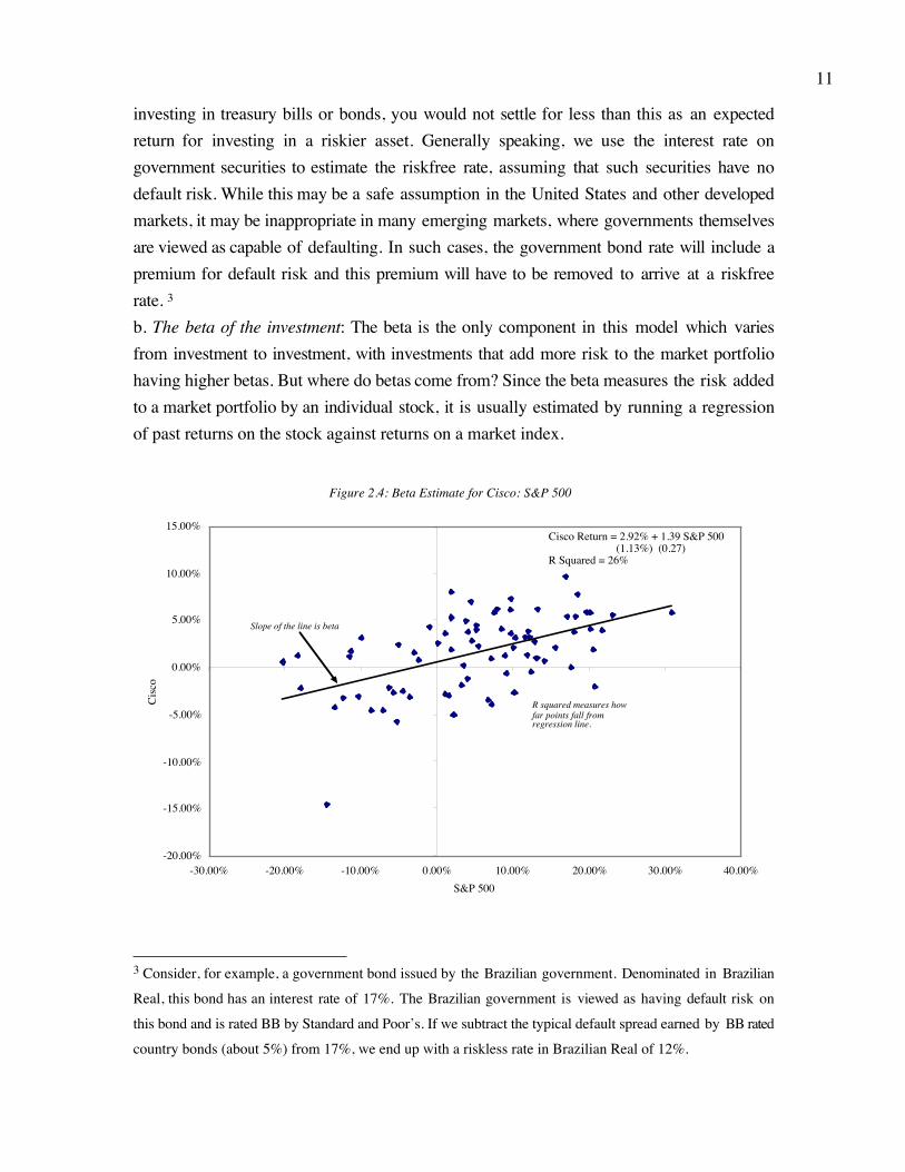
b. The beta of the investment: The beta is the only component in this model which variesfrom investment to investment, with investments that add more risk to the market portfoliohaving higher betas. But where do betas come from? Since the beta measures the risk addedto a market portfolio by an individual stock, it is usually estimated by running a regressionof past returns on the stock against returns on a market index.

Figure 2.4: Beta Estimate for Cisco: S&P 500

-20.00%

-15.00%

-10.00%

-5.00%

0.00%

5.00%

10.00%

15.00%

-30.00% -20.00% -10.00% 0.00% 10.00% 20.00% 30.00% 40.00%S&P 500

Cisc

o

Cisco Return = 2.92% + 1.39 S&P 500 (1.13%) (0.27)R Squared = 26%

Slope of the line is beta

R squared measures how far points fall from regression line.

3 Consider, for example, a government bond issued by the Brazilian government. Denominated in Brazilian

Real, this bond has an interest rate of 17%. The Brazilian government is viewed as having default risk on

this bond and is rated BB by Standard and Poor’s. If we subtract the typical default spread earned by BB rated

country bonds (about 5%) from 17%, we end up with a riskless rate in Brazilian Real of 12%.

12

Risk Premium for theUnited States: Take a look atthe equity risk premiumimplied in the U.S. stockmarket from 1960 throughthe most recent year.

The slope of the regression captures how sensitive a stock is to market movements and isthe beta of the stock. In the regression above, for instance, the beta of Cisco would be 1.39.There are, however, two problems with regression betas. One is that the beta comes withestimation error – the standard error in the estimate is 0.27. Thus, the true beta for Ciscocould be anywhere from .85 to 1.93 – this range is estimated by adding and subtracting twostandard errors to the beta estimate. The other is thatfirms change over time and we are looking backwardsrather than looking forwards. A better way to estimatebetas is to look at the average beta for publicly tradedfirms in the business or businesses Cisco operates in.While these betas come from regressions as well, theaverage beta is always more precise than any one firm’sbeta estimate.c. The risk premium for buying the average riskinvestment: You can view this as the premium you would demand for investing in equities asa class as opposed to the riskless investment. Thus, if you require a return of 9% forinvesting in equities and the treasury bond rate is 5%, your risk premium is 4%. There areagain two ways in which you can estimate this risk premium. One is to look at the past andlook at the typical premium you would have earned investing in stocks as opposed to ariskless investment. This number is called a historical premium and yields about 5-7% forthe United States. The other is to look at how stocks are priced today and to estimate thepremium that investors must be demanding. This is called an implied premium and yields avalue of about 4% for U.S. stocks in early 2002.

Bringing it all together, you could use the capital asset pricing model to estimate theexpected return on a stock for Cisco for the future (assuming a treasury bond rate of 5%,the regression beta of 1.39 and a risk premium of 4%):Expected return on Cisco = T. Bond Rate + Beta * Risk Premium

= 5% + 1.39 (4%) = 10.56%What does this number imply? It does not mean that you will earn 10.56% every year fromrisk, but it does provide a benchmark that you will have to meet and beat if you areconsidering Cisco as an investment. For Cisco to be a good investment, you would have toexpect it to make more than 10.56% as an annual return in the future.In summary, in the capital asset pricing model, all the market risk is captured in the beta,measured relative to a market portfolio, which at least in theory should include all tradedassets in the market place held in proportion to their market value.

13

Betas for Other InvestmentsMost services report betas for publicly traded stocks, but there is no reason why the

concept cannot be extended to other investments. You could compute the beta of real estate,gold or even fine art as an investment, just as you computed the beta for Cisco. Whileanalysts have done this and concluded that both real estate and gold are low betainvestments (though not necessarily low variance investments), we would add a fewcautionary notes. The first is that it is difficult to get traded prices on some alternativeinvestments on a continuous basis. 4 The second is that many analysts continue to use thestock index as their measure of the market portfolio. Since the market portfolio in the capitalasset pricing model is supposed to include all traded assets, this likely to give you betas thatare biased downwards for non-equity investments.

If you modify the market portfolio to include other traded asset classes and computebetas for alternative investments, you may even find some that have negative betas. While,on the face of it, this may seem absurd, you can get negative betas for investments thatreduce the risk (rather than add on to risk) of the market portfolio. Essentially, theseinvestments act as insurance against some large component of market risk, going up asother investments in the portfolio go down. This is the reason why some analysts claim thatgold as an investment should have a negative beta, because it tends to do well when inflationincreases whereas financial investments are hurt.

B. Alternatives to the Capital Asset Pricing ModelThe restrictive assumptions on transactions costs and private information in the

capital asset pricing model and the model’s dependence on the market portfolio have longbeen viewed with skepticism by both academics and practitioners. There are threealternatives to the CAPM that have been developed over time:1. Arbitrage Pricing Model: To understand the arbitrage pricing model, we need to beginwith a definition of arbitrage. The basic idea is a simple one. Two portfolios or assets withthe same exposure to market risk should be priced to earn exactly the same expectedreturns. If they are not, you could buy the less expensive portfolio, sell the more expensiveportfolio, have no risk exposure and earn a return that exceeds the riskless rate. This isarbitrage. If you assume that arbitrage is not possible and that investors are diversified, youcan show that the expected return on an investment should be a function of its exposure tomarket risk. While this statement mirrors what was stated in the capital asset pricing model,

4 Analysts have tried to get around this problem by using the prices of real estate investment trusts which

are traded, but they represent a small fraction of all real estate investments.

14

the arbitrage pricing model does not make the restrictive assumptions about transactionscosts and private information that lead to the conclusion that one beta can capture aninvestment’s entire exposure to market risk. Instead, in the arbitrage pricing model, you canhave multiples sources of market risk and different exposures to each (betas) and yourexpected return on an investment can be written as:

Expected return = Riskfree rate + Beta for factor 1 (Risk premium for factor 1) +Beta for factor 2 (Risk premium for factor 2)….+ Beta for factor n (Risk premiumfor factor n)

The practical questions then become knowing how many factors there are that determineexpected returns and what the betas for each investment are against these factors. Thearbitrage model estimates both by examining historical data on stock returns for commonpatterns (since market risk affects most stocks) and estimating each stock’s exposure tothese patterns in a process called factor analysis. A factor analysis provides two outputmeasures:

1. It specifies the number of common factors that affected the historical return data2. It measures the beta of each investment relative to each of the common factors andprovides an estimate of the actual risk premium earned by each factor.

The factor analysis does not, however, identify the factors in economic terms – the factorsremain factor 1, factor etc. In summary, in the arbitrage pricing model, the market risk ismeasured relative to multiple unspecified macroeconomic variables, with the sensitivity ofthe investment relative to each factor being measured by a beta. The number of factors, thefactor betas and factor risk premiums can all be estimated using the factor analysis.2. Multi-factor Models for risk and return: The arbitrage pricing model's failure toidentify the factors specifically in the model may be a statistical strength, but it is an intuitiveweakness. The solution seems simple: Replace the unidentified statistical factors withspecific economic factors and the resultant model should have an economic basis while stillretaining much of the strength of the arbitrage pricing model. That is precisely what multi-factor models try to do. Multi-factor models generally are determined by historical data,rather than economic modeling. Once the number of factors has been identified in thearbitrage pricing model, their behavior over time can be extracted from the data. Thebehavior of the unnamed factors over time can then be compared to the behavior ofmacroeconomic variables over that same period to see whether any of the variables iscorrelated, over time, with the identified factors.

For instance, Chen, Roll, and Ross (1986) suggest that the followingmacroeconomic variables are highly correlated with the factors that come out of factoranalysis: industrial production, changes in default premium, shifts in the term structure,

15

unanticipated inflation, and changes in the real rate of return. These variables can then becorrelated with returns to come up with a model of expected returns, with firm-specific betascalculated relative to each variable.

( ) ( )[ ] ( )[ ] ( )[ ]ffIIfGNPGNPf RRERRERRERRE !++!+!+= ""### ...

where

#GNP = Beta relative to changes in industrial production

E(RGNP) = Expected return on a portfolio with a beta of one on the industrial

production factor and zero on all other factors

#I = Beta relative to changes in inflation

E(RI) = Expected return on a portfolio with a beta of one on the inflation factor

and zero on all other factorsThe costs of going from the arbitrage pricing model to a macroeconomic multi-

factor model can be traced directly to the errors that can be made in identifying the factors.The economic factors in the model can change over time, as will the risk premia associatedwith each one. For instance, oil price changes were a significant economic factor drivingexpected returns in the 1970s but are not as significant in other time periods. Using thewrong factor or missing a significant factor in a multi-factor model can lead to inferiorestimates of expected return.

In summary, multi-factor models, like the arbitrage pricing model, assume thatmarket risk can be captured best using multiple macro economic factors and betas relative toeach. Unlike the arbitrage pricing model, multi factor models do attempt to identify themacro economic factors that drive market risk.

3. Regression or Proxy Models: All the models described so far begin by defining marketrisk in broad terms and then developing models that might best measure this market risk.All of them, however, extract their measures of market risk (betas) by looking at historicaldata. There is a final class of risk and return models that start with the returns and try toexplain differences in returns across stocks over long time periods using characteristics

such as a firm’s market value or price multiples5. Proponents of these models argue that ifsome investments earn consistently higher returns than other investments, they must beriskier. Consequently, we could look at the characteristics that these high-return investments

5 A price multiple is obtained by dividing the market price by its earnings or its book value. Studiesindicate that stocks that have low price to earnings multiples or low price to book value multiples earnhigher returns than other stocks.

16

have in common and consider these characteristics to be indirect measures or proxies formarket risk.

Fama and French, in a highly influential study of the capital asset pricing model inthe early 1990s, noted that actual returns between 1963 and 1990 have been highly

correlated with book to price ratios6 and size. High return investments, over this period,tended to be investments in companies with low market capitalization and high book to priceratios. Fama and French suggested that these measures be used as proxies for risk andreport the following regression for monthly returns on stocks on the NYSE:

R MV 0.35ln BVMVt = ! ( ) +$

%&

'

()1 77 0 11. % . ln

whereMV = Market Value of EquityBV/MV = Book Value of Equity / Market Value of Equity

The values for market value of equity and book-price ratios for individual firms, whenplugged into this regression, should yield expected monthly returns.

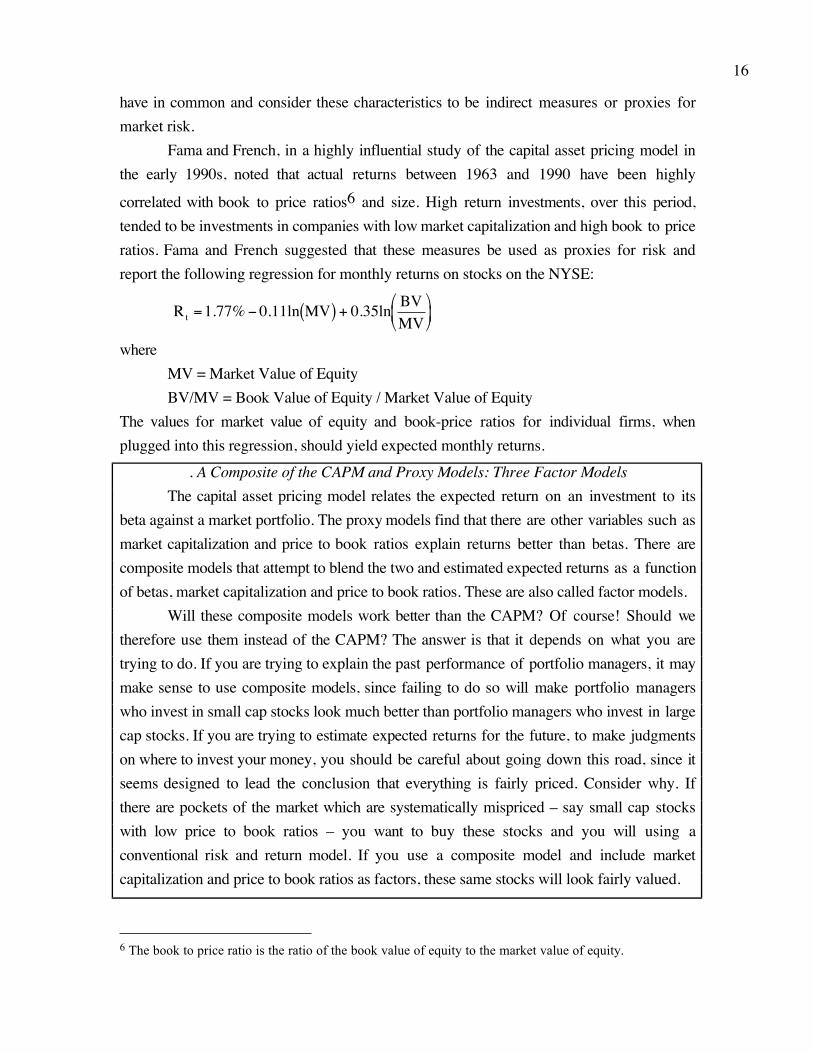
. A Composite of the CAPM and Proxy Models: Three Factor ModelsThe capital asset pricing model relates the expected return on an investment to its

beta against a market portfolio. The proxy models find that there are other variables such asmarket capitalization and price to book ratios explain returns better than betas. There arecomposite models that attempt to blend the two and estimated expected returns as a functionof betas, market capitalization and price to book ratios. These are also called factor models.

Will these composite models work better than the CAPM? Of course! Should wetherefore use them instead of the CAPM? The answer is that it depends on what you aretrying to do. If you are trying to explain the past performance of portfolio managers, it maymake sense to use composite models, since failing to do so will make portfolio managerswho invest in small cap stocks look much better than portfolio managers who invest in largecap stocks. If you are trying to estimate expected returns for the future, to make judgmentson where to invest your money, you should be careful about going down this road, since itseems designed to lead the conclusion that everything is fairly priced. Consider why. Ifthere are pockets of the market which are systematically mispriced – say small cap stockswith low price to book ratios – you want to buy these stocks and you will using aconventional risk and return model. If you use a composite model and include marketcapitalization and price to book ratios as factors, these same stocks will look fairly valued.

6 The book to price ratio is the ratio of the book value of equity to the market value of equity.

17

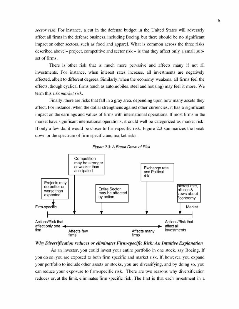
A Comparative Analysis of Risk and Return ModelsFigure 2.5 summarizes all the risk and return models in finance, noting their

similarities in the first two steps and the differences in the way they define market risk.

Figure 2.5: Risk and Return Models in Finance

The risk in an investment can be measured by the variance in actual returns around an expected return

E(R)

Riskless Investment Low Risk Investment High Risk Investment

E(R) E(R)

Risk that is specific to investment (Firm Specific) Risk that affects all investments (Market Risk)Can be diversified away in a diversified portfolio Cannot be diversified away since most assets1. each investment is a small proportion of portfolio are affected by it.2. risk averages out across investments in portfolioThe marginal investor is assumed to hold a “diversified” portfolio. Thus, only market risk will be rewarded and priced.

The CAPM The APM Multi-Factor Models Proxy ModelsIf there is 1. no private information2. no transactions costthe optimal diversified portfolio includes everytraded asset. Everyonewill hold this market portfolioMarket Risk = Risk added by any investment to the market portfolio:

If there are no arbitrage opportunities then the market risk ofany asset must be captured by betas relative to factors that affect all investments.Market Risk = Risk exposures of any asset to market factors

Beta of asset relative toMarket portfolio (froma regression)

Betas of asset relativeto unspecified marketfactors (from a factoranalysis)

Since market risk affectsmost or all investments,it must come from macro economic factors.Market Risk = Risk exposures of any asset to macro economic factors.

Betas of assets relativeto specified macroeconomic factors (froma regression)

In an efficient market,differences in returnsacross long periods mustbe due to market riskdifferences. Looking forvariables correlated withreturns should then give us proxies for this risk.Market Risk = Captured by the Proxy Variable(s)

Equation relating returns to proxy variables (from aregression)

Step 1: Defining Risk

Step 2: Differentiating between Rewarded and Unrewarded Risk

Step 3: Measuring Market Risk

As noted in Figure 2.5, all the risk and return models developed in this chapter makesome assumptions in common. They all assume that only market risk is rewarded and theyderive the expected return as a function of measures of this risk. The capital asset pricingmodel makes the most restrictive assumptions about how markets work but arrives at thesimplest model, with only one factor driving risk and requiring estimation. The arbitragepricing model makes fewer assumptions but arrives at a more complicated model, at least interms of the parameters that require estimation. The capital asset pricing model can beconsidered a specialized case of the arbitrage pricing model, where there is only oneunderlying factor and it is completely measured by the market index. In general, the CAPMhas the advantage of being a simpler model to estimate and to use, but it will underperformthe richer multi-factor models when an investment is sensitive to economic factors not wellrepresented in the market index. For instance, oil company stocks, which derive most of

18

their risk from oil price movements, tend to have low CAPM betas and low expectedreturns. An arbitrage pricing model, where one of the factors may measure oil and othercommodity price movements, will yield a better estimate of risk and higher expected return

for these firms7.Which of these models works the best? Is beta a good proxy for risk and is it

correlated with expected returns? The answers to these questions have been debated widelyin the last two decades. The first tests of the CAPM suggested that betas and returns werepositively related, though other measures of risk (such as variance) continued to explaindifferences in actual returns. This discrepancy was attributed to limitations in the testingtechniques. In 1977, Roll, in a seminal critique of the model's tests, suggested that since themarket portfolio could never be observed, the CAPM could never be tested, and all tests ofthe CAPM were therefore joint tests of both the model and the market portfolio used in thetests. In other words, all that any test of the CAPM could show was that the model worked(or did not) given the proxy used for the market portfolio. It could therefore be argued thatin any empirical test that claimed to reject the CAPM, the rejection could be of the proxyused for the market portfolio rather than of the model itself. Roll noted that there was noway to ever prove that the CAPM worked and thus no empirical basis for using the model.

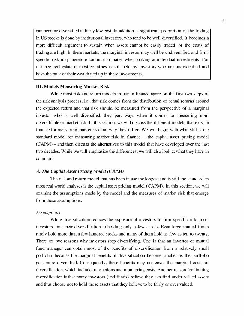
Fama and French (1992) examined the relationship between betas and returnsbetween 1963 and 1990 and concluded that there is no relationship. These results have beencontested on three fronts. First, Amihud, Christensen, and Mendelson (1992), used the samedata, performed different statistical tests and showed that differences in betas did, in fact,explain differences in returns during the time period. Second, Kothari and Shanken (1995)estimated betas using annual data, instead of the shorter intervals used in many tests, andconcluded that betas do explain a significant proportion of the differences in returns acrossinvestments. Third, Chan and Lakonishok (1993) looked at a much longer time series ofreturns from 1926 to 1991 and found that the positive relationship between betas andreturns broke down only in the period after 1982. They also find that betas are a usefulguide to risk in extreme market conditions, with the riskiest firms (the 10% with highestbetas) performing far worse than the market as a whole, in the ten worst months for themarket between 1926 and 1991 (See Figure 2.6).

7 Weston and Copeland used both approaches to estimate the cost of equity for oil companies in 1989 andcame up with 14.4% with the CAPM and 19.1% using the arbitrage pricing model.

19

FIGURE 2.6: Returns and Betas: Ten Worst Months between 1926 and 1991

Mar

198

8

Oct

198

7

May

194

0

May

193

2

Apr

193

2

Sep

193

7

Feb

193

3

Oct

193

2

Mar

198

0

Nov

197

3

High-beta stocks Whole Market Low-beta stocks

While the initial tests of the APM suggested that they might provide more promisein terms of explaining differences in returns, a distinction has to be drawn between the useof these models to explain differences in past returns and their use to predict expectedreturns in the future. The competitors to the CAPM clearly do a much better job atexplaining past returns since they do not constrain themselves to one factor, as the CAPMdoes. This extension to multiple factors does become more of a problem when we try toproject expected returns into the future, since the betas and premiums of each of thesefactors now have to be estimated. Because the factor premiums and betas are themselvesvolatile, the estimation error may eliminate the benefits that could be gained by moving fromthe CAPM to more complex models. The regression models that were offered as analternative also have an estimation problem, since the variables that work best as proxies formarket risk in one period (such as market capitalization) may not be the ones that work inthe next period.

Ultimately, the survival of the capital asset pricing model as the default model forrisk in real world applications is a testament to both its intuitive appeal and the failure ofmore complex models to deliver significant improvement in terms of estimating expectedreturns. We would argue that a judicious use of the capital asset pricing model, without anover reliance on historical data, is still the most effective way of dealing with risk in moderncorporate finance.

20

Models of Default RiskThe risk that we have discussed hitherto in this chapter relates to cash flows on

investments being different from expected cash flows. There are some investments, however,in which the cash flows are promised when the investment is made. This is the case, forinstance, when you lend to a business or buy a corporate bond. However, the borrower maydefault on interest and principal payments on the borrowing. Generally speaking, borrowerswith higher default risk should pay higher interest rates on their borrowing than those withlower default risk. This section examines the measurement of default risk and therelationship of default risk to interest rates on borrowing.

In contrast to the general risk and return models for equity, which evaluate theeffects of market risk on expected returns, models of default risk measure the consequencesof firm-specific default risk on promised returns. While diversification can be used toexplain why firm-specific risk will not be priced into expected returns for equities, the samerationale cannot be applied to securities that have limited upside potential and much greaterdownside potential from firm-specific events. To see what we mean by limited upsidepotential, consider investing in the bond issued by a company. The coupons are fixed at thetime of the issue and these coupons represent the promised cash flow on the bond. The bestcase scenario for you as an investor is that you receive the promised cash flows; you are notentitled to more than these cash flows even if the company is wildly successful. All otherscenarios contain only bad news, though in varying degrees, with the delivered cash flowsbeing less than the promised cash flows. Consequently, the expected return on a corporatebond is likely to reflect the firm-specific default risk of the firm issuing the bond.

The Determinants of Default RiskThe default risk of a firm is a function of two variables. The first is the firm’s

capacity to generate cash flows from operations and the second is its financial obligations –

including interest and principal payments8. Firms that generate high cash flows relative totheir financial obligations should have lower default risk than firms that generate low cashflows relative to their financial obligations. Thus, firms with significant existing investments,which generate relatively high cash flows, will have lower default risk than firms that do not.

In addition to the magnitude of a firm’s cash flows, the default risk is also affected bythe volatility in these cash flows. The more stability there is in cash flows the lower the

8 Financial obligation refers to any payment that the firm has legally obligated itself to make, such asinterest and principal payments. It does not include discretionary cash flows, such as dividend payments ornew capital expenditures, which can be deferred or delayed, without legal consequences, though there maybe economic consequences.

21

default risk in the firm. Firms that operate in predictable and stable businesses will havelower default risk than will other similar firms that operate in cyclical or volatile businesses.

Most models of default risk use financial ratios to measure the cash flow coverage (i.e.,the magnitude of cash flows relative to obligations) and control for industry effects toevaluate the variability in cash flows.

Bond Ratings and Interest ratesThe most widely used measure of a firm's default risk is its bond rating, which is

generally assigned by an independent ratings agency. The two best known are Standard andPoor’s and Moody’s. Thousands of companies are rated by these two agencies and theirviews carry significant weight with financial markets.

The Ratings ProcessThe process of rating a bond usually starts when the issuing company requests a

rating from a bond ratings agency. The ratings agency then collects information from bothpublicly available sources, such as financial statements, and the company itself and makes adecision on the rating. If the company disagrees with the rating, it is given the opportunity topresent additional information. This process is presented schematically for one ratingsagency, Standard and Poors (S&P), in Figure 2.7.

22

Figure 2.7: The Ratings Process

Issuer or authorized representative request rating

Requestor completes S&P rating request form and issue is entered into S&P's administrative and control systems.

S&P assigns analytical team to issue

Analysts research S&P library, internal files and data bases

Issuer meeting: presentation to S&P personnel orS&P personnel tour issuer facilities

Final Analyticalreview and preparationof rating committeepresentation

Presentation of the analysis to the S&P rating commiteeDiscussion and vote to determine rating

Notification of rating decision to issuer or its authorized representative

Does issuer wish to appeal by furnishing additional information?

Presentation of additional information to S&P rating committee: Discussion and vote to confirm or modify rating.

Format notification to issuer or its authorized representative: Rating is releasedYes

No

THE RATINGS PROCESS

23

The ratings assigned by these agencies are letter ratings. A rating of AAA from Standardand Poor’s and Aaa from Moody’s represents the highest rating granted to firms that areviewed as having the lowest default risk. As the default risk increases, the ratings decreasetoward D for firms in default (Standard and Poor’s). A rating at or above BBB by Standardand Poor’s is categorized as investment grade, reflecting the view of the ratings agency thatthere is relatively little default risk in investing in bonds issued by these firms.

Determinants of Bond RatingsThe bond ratings assigned by ratings agencies are primarily based upon publicly

available information, though private information conveyed by the firm to the rating agencydoes play a role. The rating assigned to a company's bonds will depend in large part onfinancial ratios that measure the capacity of the company to meet debt payments andgenerate stable and predictable cash flows. While a multitude of financial ratios exist, table2.1 summarizes some of the key ratios used to measure default risk.

Table 2.1: Financial Ratios used to measure Default Risk

Ratio Description

Pretax Interest

CoveragePretax Income from Continuing Operations Interest Expense

Gross Interest+

EBITDA Interest

Coverage Interest GrossEBITDA

Funds from

Operations / Total

Debt

Net Income from Continuing Operations DepreciationTotal Debt

+

Free Operating

Cashflow/ Total DebtFunds from Operations - Capital Expenditures-Change in Working Capital

Total Debt

$

%&

'

()

Pretax Return on

Permanent CapitalPretax Income from Continuing Operations Interest Expense

Average of Beginning of the year and End of the year of long andshort term debt, minority interest and Shareholders Equity

+$

%&

'

()

Operating

Income/SalesSales - COGS(before depreciation) -Selling Expenses -Administrative Expenses - R & D Expenses

Sales

$

%&

'

()

24

Companies with AAAratings: Take a look at thecompanies that commandedtriple AAA ratings fromStandard and Poor’s in themost recent period.

Long Term Debt/

CapitalLong Term Debt

Long Term Debt Equity

+

Total

Debt/CapitalizationTotal Debt

Total Debt Equity+

Source: Standard and PoorsThere is a strong relationship between the bond rating a company receives and its

performance on these financial ratios. Table 2.2 provides a summary of the median ratios9

from 1998 to 2000 for different S&P ratings classes for manufacturing firms.Table 2.2: Financial Ratios by Bond Rating: 1998-2000

AAA AA A BBB BB B CCC

EBIT interest cov. (x) 17.5 10.8 6.8 3.9 2.3 1.0 0.2

EBITDA interest cov. 21.8 14.6 9.6 6.1 3.8 2.0 1.4

Funds flow/total debt 105.8 55.8 46.1 30.5 19.2 9.4 5.8

Free oper. cash

flow/total debt (%)

55.4 24.6 15.6 6.6 1.9 –4.5 -14.0

Return on capital (%) 28.2 22.9 19.9 14.0 11.7 7.2 0.5

Oper.income/sales

(%)

29.2 21.3 18.3 15.3 15.4 11.2 13.6

Long-term

debt/capital (%)

15.2 26.4 32.5 41.0 55.8 70.7 80.3

Total Debt/ Capital

(%)

26.9 35.6 40.1 47.4 61.3 74.6 89.4

Number of firms 10 34 150 234 276 240 23

Source: Standard and Poors

Note that the pre-tax interest coverage ratio (EBIT) and the EBITDA interest coverage ratioare stated in terms of times interest earned, whereas the rest of the ratios are stated inpercentage terms.

Not surprisingly, firms that generate income andcash flows significantly higher than debt payments, thatare profitable and that have low debt ratios are more likely

9 See the Standard and Poor’s online site: http://www.standardandpoors.com/ratings/criteria/index.htm

25

to be highly rated than are firms that do not have these characteristics. There will beindividual firms whose ratings are not consistent with their financial ratios, however, becausethe ratings agency does add subjective judgments into the final mix. Thus, a firm thatperforms poorly on financial ratios but is expected to improve its performance dramaticallyover the next period may receive a higher rating than is justified by its current financials.For most firms, however, the financial ratios should provide a reasonable basis for guessingat the bond rating.

Synthetic Ratings and Default RiskNot all firms that borrow money have bond ratings available on them. How do you

go about estimating the cost of debt for these firms? There are two choices.• One is to look at recent borrowing history. Many firms that are not rated still borrow

money from banks and other financial institutions. By looking at the most recentborrowings made by a firm, you can get a sense of the types of default spreads beingcharged the firm and use these spreads to come up with a cost of debt.

• The other is to estimate a synthetic rating for the firm, i.e, use the financial ratios usedby the bond ratings agencies to estimate a rating for the firm. To do this you would needto begin with the rated firms and examine the financial characteristics shared by firmswithin each ratings class. As an example, assume that you have an unrated firm withoperating earnings of $ 100 million and interest expenses of $ 20 million. You coulduse the interest coverage ratio of 5.00 (100/20) to estimate a bond rating of A- for this

firm.10.

Bond Ratings and Interest RatesThe interest rate on a corporate bond should be a function of its default risk, which

is measured by its rating. If the rating is a good measure of the default risk, higher ratedbonds should be priced to yield lower interest rates than would lower rated bonds. Thedifference between the interest rate on a bond with default risk and a default-freegovernment bond is defined to be the default spread. Table 2.3 summarizes default spreadsfor 10-year bonds in S&P’s different rating classes as of December 31, 2001:

Table 2.3: Default Spreads and Bond RatingsRating Spread

10 This rating was based upon a table that was developed in 1999 and 2000, by listing out all rated firms,with market capitalization lower than $ 2 billion, and their interest coverage ratios, and then sorting firmsbased upon their bond ratings. The ranges were adjusted to eliminate outliers and to prevent overlappingranges.

26

AAA 0.75%AA 1.00%A+ 1.50%A 1.80%A- 2.00%

BBB 2.25%BB 3.50%B+ 4.75%B 6.50%B- 8.00%

CCC 10.00%CC 11.50%C 12.70%D 14.00%

Source: www.bondsonline.com

These default spreads, when added to the riskless rate, yield the interest rates forbonds with the specified ratings. For instance, a D rated bond has an interest rate about 14%higher than the riskless rate. This default spread will vary by maturity of the bond and canalso change from period to period, depending on economic conditions, widening duringeconomic slowdowns and narrowing when the economy is strong.

SummaryRisk, as we define it in finance, is measured based upon deviations of actual returns

on an investment from its' expected returns. There are two types of risk. The first, which wecall equity risk, arises in investments where there are no promised cash flows, but there areexpected cash flows. The second, default risk, arises on investments with promised cashflows.

On investments with equity risk, the risk is best measured by looking at the varianceof actual returns around the expected returns, with greater variance indicating greater risk.This risk can be broken down into risk that affects one or a few investments, which we callfirm specific risk, and risk that affects many investments, which we refer to as market risk.When investors diversify, they can reduce their exposure to firm specific risk. By assumingthat the investors who trade at the margin are well diversified, we conclude that the risk weshould be looking at with equity investments is the market risk. The different models ofequity risk introduced in this chapter share this objective of measuring market risk, but they

27

differ in the way they do it. In the capital asset pricing model, exposure to market risk ismeasured by a market beta, which estimates how much risk an individual investment willadd to a portfolio that includes all traded assets. The arbitrage pricing model and the multi-factor model allow for multiple sources of market risk and estimate betas for an investmentrelative to each source. Regression or proxy models for risk look for firm characteristics,such as size, that have been correlated with high returns in the past and use these to measuremarket risk. In all these models, the risk measures are used to estimate the expected returnon an equity investment. This expected return can be considered the cost of equity for acompany.

On investments with default risk, risk is measured by the likelihood that thepromised cash flows might not be delivered. Investments with higher default risk shouldhave higher interest rates and the premium that we demand over a riskless rate is the defaultpremium. For most US companies, default risk is measured by rating agencies in the formof a company rating; these ratings determine, in large part, the interest rates at which thesefirms can borrow. Even in the absence of ratings, interest rates will include a defaultpremium that reflects the lenders’ assessments of default risk. These default-risk adjustedinterest rates represent the cost of borrowing or debt for a business.

28

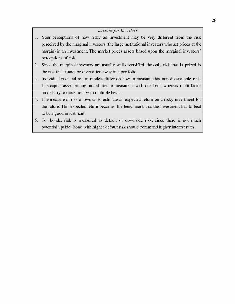
Lessons for Investors1. Your perceptions of how risky an investment may be very different from the risk

perceived by the marginal investors (the large institutional investors who set prices at themargin) in an investment. The market prices assets based upon the marginal investors’perceptions of risk.

2. Since the marginal investors are usually well diversified, the only risk that is priced isthe risk that cannot be diversified away in a portfolio.

3. Individual risk and return models differ on how to measure this non-diversifable risk.The capital asset pricing model tries to measure it with one beta, whereas multi-factormodels try to measure it with multiple betas.

4. The measure of risk allows us to estimate an expected return on a risky investment forthe future. This expected return becomes the benchmark that the investment has to beatto be a good investment.

5. For bonds, risk is measured as default or downside risk, since there is not muchpotential upside. Bond with higher default risk should command higher interest rates.