4

CHAPTER 2 - THE PLUS-MINUS TIME ANALYSIS METHOD

2.1 INTRODUCTION

2.1.1 Purpose of the method

The Plus-Minus time analysis method has two objectives: to establish a near-surface

model of the Earth in terms of subweathering layer thicknesses and seismic wave velocities;

and to compute static corrections to be applied to seismic data. The surface layers of the

Earth are often made of unconsolidated deposits or soil which have low seismic velocities.

For example, in Western Canada the near-surface layers are generally composed of

Quaternary glacial deposits (Clague, 1991), while in South America or Africa the surface

layers are made of weathered soil materials. These low velocity layers will induce

recording delays of seismic reflection data. The impact of these delays on reflector

structure can be quite significant. The use of seismic refracted arrivals to establish the

thicknesses of these layers and their seismic wave velocities represents one of the best

ways to correct for these delays.

2.1.2 Theory

The refraction analysis method used is the “plus-minus” method of Hagedoorn (1959),

which includes the Plus time analysis for depth analysis and the Minus time analysis for

velocity determination (van Overmeeran, 1987). The basis of the Plus-Minus time analysis

method lies in the traveltime reciprocity, i.e. the traveltime of a seismic wave from source

to receiver is equal to the traveltime in the opposite direction if source and receiver are

interchanged. The Plus time analysis uses the concept of the Delay time analysis

introduced by Gardner (1939, 1967) and further developed by Hawkins (1961) and Barry

(1967) (see Delay time analysis in Appendix A). The basic geometry of the Plus-Minus

time analysis method is illustrated in Figure 2.1.

To be able to use the Plus time analysis, reciprocal spread data are essential so that the

forward arrival spread extends at least to the position of the reverse source (Sr) and the

reverse arrival spread to the position of the forward source (Sf) (Figure 2.1). The Plus-

Minus time analysis window is defined by the two crossover points (forward spread (Xf)

and reverse spread (Xr)), which determine the offset limit between the first layer arrivals

and the second layer arrivals.

5

A

B

v1

v2

C

D

E F G

H

θCθC

Dep

th

Z1D

TAH

THDTAD

THA

Tra

vel

tim

e

Coordinate

Plus-Minus Time analysis window

Sf S rXf XrD

θCθCθC

Figure 2.1. Plus time analysis according to the “plus-minus” method of Hagedoorn(1959).

The Plus time value (T+) can be evaluated for each of the receivers inside that window.

The Plus time value at a receiver (T+D) is defined (Hagedoorn, 1959) as the sum of the

traveltime at the receiver from a forward source (TAD) and the traveltime at the receiver

from the reverse source (THD), minus the traveltime between the two sources (TAH).

T+D = TAD + THD - TAH (2.1)

6After some substitution in Equation (2.1) and knowing that the Delay time at receiver D

(δD) is equal to half the Plus time (T+D) at the same receiver, a relation with the thickness

(Z1D) of the first layer below the receiver can be found.

Z1D = [(T+D)*(V

1)]/2(cos(θc)) (2.2)

where θc =sin-1(V

1/V

2), V

1 and V

2 are respectively the first and second layer velocities.

The velocity of the first layer can be found using the inverse slope of the first layer

arrivals (Sf to Xf and Sr to Xr). From the second layer arrivals (after Xf for the forward

spread and after Xr for the reverse spread), the second layer velocity can be derived using

the Minus time analysis (Figure 2.2).

A

B

v1

v2

C

D

F G

H

Dep

th

D'

C' F'

X

Figure 2.2. Minus time analysis according to the “plus-minus” method of Hagedoorn(1959).

The definition of the Minus time (T-D) at a receiver is the subtraction of the traveltime at

the receiver from the reverse source (THD) of the traveltime at the receiver from the

forward source (TAD), minus the traveltime between the two sources (TAH).

T-D = TAD - THD - TAH (2.3)

A velocity analysis of the second layer can be undertaken using the Minus time values at

two receivers (D and D') with a specified separation distance (∆X).

7

T-D' -T-D = ∆T-D = 2(∆X)/V2

(2.4)

The velocity of the second layer (V2) is equal to twice the inverse slope of a best fit line

through the Minus time variations (∆T-D) calculated for receivers inside the Plus-Minus

time analysis window.

V2= 2(∆X)/∆T-D (2.5)

Summary

Knowing the Plus time values, the first and second layer velocities at each receiver, the

thickness of the first layer below each receiver can be found according to the Delay time

analysis. For more details about the Plus time and Minus time analyses, see Appendix B.

The Delay time represents the time to travel from the receiver to the refractor minus the time

necessary to travel the normal projection of the raypath on the refractor (Figure 2.1). From

Snell's law, a relation between the Delay times and the thickness of the first layer at the

receiver can be established. Finally, the link between the Delay times and the Plus times

allows us to determine the thickness of the first layer below each receivers inside the Plus-

Minus time analysis window (Equation 2.2). This will allow the determination of the first

layer thickness all along a seismic survey line. Therefore, this analysis is restricted to a

two layer case in two dimensions. The first layer velocity can be evaluated using a

polynomial fit of the direct arrival or a rough estimate of the subweathering layer (first

layer). The knowledge of the first layer thickness and velocity allows the determination of

surface-consistent weathering static corrections, where the replacement velocity is the

average refractor velocity.

2.1.3 Hardware/software requirement

The Plus-Minus time analysis software is written in the Matlab language. Matlab is a

commercial package which provides a technical computing and visualization environment.

A Matlab license is required to run the Plus-Minus time analysis software. Currently,

arrival times and geometry are input from ProMax exported database files. The refracted

arrival times are previously picked in the processing software (currently ProMax) and then

input to the Plus-Minus time analysis software. The geometry files include the receiver

coordinates and elevations, and the shot coordinates and elevations, as well as the uphole

time (see data files section in Appendix C). The software can be run on any platform for

8which Matlab is available, including UNIX, MS-Windows, and Macintosh (see PMT

method implementation in Appendix C).

2.2 PROCESS

2.2.1 General flow chart

The Plus-Minus time analysis method developed for this thesis consists of seven major

steps and four optional steps (Figure 2.3). As explained in the data file section (Appendix

C), the refracted arrivals and the geometry files are required to properly initiate the

processing. There are three final results of processing; a velocity model, a depth model,

and the static corrections.

After the data are loaded, the inflection points on the refracted arrivals are identified.

These are called crossover points (CVPs). The crossover points represent a change in the

first arrival times between the first layer arrivals and the second layer arrivals. Once the

locations of the crossover points are known for each source arrival spread, the velocities of

the first layer can be calculated using a polynomial fit of the direct arrivals. The second

layer velocities are calculated using the Minus time analysis with the refracted arrivals.

Simultaneously, the time delays caused by the downgoing and upgoing refracted wave

raypath through the first layer can be determined using Plus time and Delay time analyses

of the refracted arrivals. Once the Plus times and the two layer velocities are known, the

first layer thicknesses are computed in the depth calculation processing step. Finally, from

the first layer thicknesses and velocities, the static corrections which determine the effect of

that layer, can be found using the static computation processing step.

9

VELOCITY MODEL

STATIC CORRECTIONS

DEPTH MODEL

STATIC COMPUTATION

DEPTH CALCULATION

PLUS TIME REJECTION

PLUS TIME & DELAY TIMEANALYSES

VELOCITY CALCULATION

REFRACTED ARRIVALS & GEOMETRY FILES

LOAD DATA

RECIPROCAL TIME CHECK

CROSSOVER POINT AUTOPICKING

CROSSOVER POINT REJECTION

CROSSOVER POINT AVERAGING

POLYFIT & CROSSOVER POINT REPICKING

Figure 2.3. Processing flow chart

102.2.2 Reciprocal time check

As mentioned in the theory section, the basis of the Plus-Minus time analysis method

lies in the traveltime reciprocity, i.e. the traveltime of a seismic wave between two locations

in one direction is equal to the traveltime in the opposite direction. For example, if seismic

energy is sent from a shot and recorded at a certain distance by a receiver, the shot and

receiver position may be switched, but the traveltime recorded in both cases should be

equal.

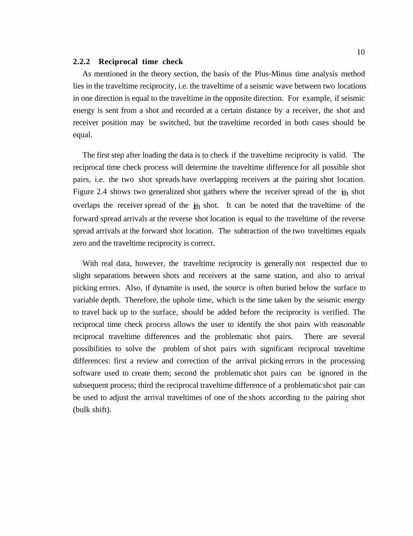
The first step after loading the data is to check if the traveltime reciprocity is valid. The

reciprocal time check process will determine the traveltime difference for all possible shot

pairs, i.e. the two shot spreads have overlapping receivers at the pairing shot location.

Figure 2.4 shows two generalized shot gathers where the receiver spread of the ith shot

overlaps the receiver spread of the jth shot. It can be noted that the traveltime of the

forward spread arrivals at the reverse shot location is equal to the traveltime of the reverse

spread arrivals at the forward shot location. The subtraction of the two traveltimes equals

zero and the traveltime reciprocity is correct.

With real data, however, the traveltime reciprocity is generally not respected due to

slight separations between shots and receivers at the same station, and also to arrival

picking errors. Also, if dynamite is used, the source is often buried below the surface to

variable depth. Therefore, the uphole time, which is the time taken by the seismic energy

to travel back up to the surface, should be added before the reciprocity is verified. The

reciprocal time check process allows the user to identify the shot pairs with reasonable

reciprocal traveltime differences and the problematic shot pairs. There are several

possibilities to solve the problem of shot pairs with significant reciprocal traveltime

differences: first a review and correction of the arrival picking errors in the processing

software used to create them; second the problematic shot pairs can be ignored in the

subsequent process; third the reciprocal traveltime difference of a problematic shot pair can

be used to adjust the arrival traveltimes of one of the shots according to the pairing shot

(bulk shift).

11

i j

Figure 2.4. Reciprocal time check with shot gathers i and j.

2.2.3 Crossover point autopicking

Crossover point picking represents the most important step of this program. The

crossover points indicate a change in the arrivals between the first and second layer. At the

crossover point, the traveltime of the second layer arrivals is equal to the traveltime of the

first layer arrivals. Beyond the crossover point, the refracted arrivals from the second layer

are recorded before the first layer arrivals. The first layer arrivals (also called direct

arrivals) are the traveltimes of a seismic wave from the source to the receivers along the

surface of the first layer. The second layer arrivals (also called refracted arrivals) are the

traveltimes of a seismic wave from the source to the bottom of the first layer then along the

first and second layer interface and back up through the first layer to the receivers (Figure

2.5).

The position of the crossover points on each shot spread is found using the traveltime

difference analysis developed by Lawton (1989) and the branch point analysis of Wang and

Cheadle (1995). The traveltime difference analysis consists of subtracting two adjacent

shot arrival traveltimes at common receiver locations (Figure 2.6). The traveltime

differences (δt) remain constant when the arrivals from the two shots involve the same

layer. The crossover point is located at the limit between a constant traveltime difference

12and an increasing or decreasing traveltime difference. For example, if we subtract the

traveltime of two overlapping shot gathers (Figure 2.6), it can be noticed that the traveltime

difference on the left of shot i location is constant until it reaches the left crossover point of

the shot gather i and then the traveltime difference increases. On the other side (right of

shot j location), the traveltime difference decreases until it reaches the right crossover point

of shot gather j and then remains constant. Then, if we calculate the first and second

derivatives of the traveltime differences, the crossover point locations correspond to the

maximum value of the second derivative. This result is due to a maximum change of slope

on the traveltime differences at the first and second layer inflection point and allows

automatic crossover point location picking for each overlapping shot pair spread. The use

of all possible overlapping shot pairs allows not only the identification of the crossover

point (left and/or right) on each shot gather but also a statistically redundant crossover point

location on the same shot spread (left or right).

Another important feature of the traveltime difference analysis is the cancellation of

traveltime irregularities due to topographic features. However, in the real data case,

traveltime irregularities can also be due to errors in the arrival picking and other

instrumental factors, so that filtering is essential. A median filter is first applied to the

traveltime difference to remove high-frequency variation and keep the general trend of the

traveltime difference, especially the step trend at the crossover point. After the first

derivative is calculated, a mean filter can be applied to smooth the short wavelength

variations due to small steps in the median filtered traveltime difference curve, and keep the

long wavelength variation due to major steps associated with the crossover point locations.

The mean filter should be used with care and only if the first derivative curve appears

noisy. The window length of these filters is determined by the user and should be tested

on each dataset. Also, the first and second derivatives use a parameter called differentiation

separation length, which can be defined by the user. This parameter determines the number

of samples in between each subtraction for the derivation. For example if one is used the

differentiation of the traveltime difference curve corresponds to its simple derivative, i.e.

the sample interval is one.

∆t/∆x = [t(x + n∆s) - t(x)]/n∆s (2.6)

where x and ∆x are respectively the coordinate of the arrival and the coordinate variation; t

and ∆t are respectively the time of the arrival and the time variation; and ∆s is the distance

of a sample interval, while n is the differentiation separation length factor.

13

The window filter length and the differentiation separation length need to be tested on

each different dataset to optimize the crossover point autopicking consistency. This will

reduce the amount of manual editing of the crossover points.

Finally, the user can specify an offset range in which the crossover points can be

picked. This feature should be used only if the user has sufficient knowledge of the data

(near-surface geology, previous identification of some crossover points throughout the

entire survey) and can confine the crossover points within a certain offset range from the

shot locations. It can also be used if third layer arrivals are suspected at a larger offsets, so

that the crossover points might be divided between the first and second layer inflections and

the second and third layer inflections. In both cases, the offset range limitation will enable

consistent crossover point picking and will save a lot of manual editing.

Surface

Layer 1

Layer 2

V1

V2

Shot (i)Receivers +

Refractedraypath

Directraypath

+

++

+ + +

++

++

+++ +

+

Coordinate

Ele

vatio

n

Interface

Figure 2.5. Direct and refracted raypath for shot gather i.

14

i j

δt

Figure 2.6. Crossover point autopicking of the left crossover point for shot gathers i (o)and of the right crossover point for shot gather j (*), according to the traveltime differenceanalysis by Lawton (1989) and the branch point analysis of Wang and Cheadle (1995).

2.2.3 Crossover point rejection

This optional process is based on the statistics of the crossover points previously

picked. As mentioned in the above section, the use of all possible overlapping shot pairs

brings an over determination of the crossover point on a shot spread. The next step is to

average all the crossover points that belong to the same shot spread (forward or reverse)

and use that value in the subsequent process. The subtraction of each possible overlapping

shot spread with a common shot spread should result in consistent traveltime differences

and same crossover point surface location. However, if the arrivals are inconsistent and

15noisy due picking problem, the traveltime difference of each overlapping shot spreads

might result in different crossover point locations. The utility of the crossover point

rejection is to identify and remove the crossover point picks for a given shot spread that

have a high deviation from the average crossover point value.

The rejection can be based on a fraction of the standard deviation of the crossover point

picks for each shot spread or on a constant deviation limit. The difference between the two

rejection limits is that the fraction of the standard deviation limit changes for each crossover

point shot spread (right or left) and the constant deviation limit remains constant for all

crossover point shot spreads. In both cases, the use of the crossover point statistics, which

includes the standard deviation, the fold and the value of the crossover point averages, is

recommended to determine the rejection limit. The user should look not only at the average

crossover point values, but at the standard deviation and at the fold of each crossover point

average. The combination of a high standard deviation with a low fold indicates a

crossover point autopicking problem and manual editing might be required, while a low

standard deviation with either a high or low fold generally indicates a successful crossover

point autopick. In the case of a high standard deviation and a high fold, the crossover point

autopicking was noisy, and the crossover point rejection might help remove some bad

crossover picks. One thing to keep in mind is that each time crossover point rejection is

used, the redundancy (fold) of the crossover point averages is reduced.

2.2.4 Crossover point averaging

The next major step after the crossover point autopicking is the averaging of all the

crossover points for a shot spread (left and/or right). For a shot with a leading (right) and a

trailing (left) spread, two individual averaging processes are required; one for the left

crossover points and one for the right crossover points. In Figure 2.7, the left crossover

points of shot gather j comes from the traveltime difference analysis of its left (trailing)

spread with all overlapping left shot spreads to its right, whereas in Figure 2.8, the right

crossover points of shot gather j come from the traveltime analysis of its right (leading)

spread with all the overlapping right shot spreads to its left. The proper crossover point

positioning is important for the velocity calculation and the Plus time analysis. The

crossover points can be edited individually before the crossover point averages are

computed. The crossover point averages can also be edited (see PMT method

implementation in Appendix C).

16

left cross overpoint (shot j)

j srqponmlk

Figure 2.7. Left crossover point determination for shot gather j, established from theoverlapping shot spread to the right .

right cross overpoint (shot j)

jihgfedcba

Figure 2.8. Right crossover point determination for shot gather j, established from theoverlapping shot spread to the left.

172.2.5 Polyfit and crossover point repicking

This optional process has the objective of obtaining a better crossover point consistency

between shot spreads. In fact, the offset distance of the crossover point average of a shot

spread from the shot location should not be too different than the offset distance of the

crossover point average on the next shot spread from its location. The offset distances

between the crossover point averages and their shot locations reveal the general shape of

the first layer thickness. Generally, the offset varies proportionally with the variation of the

first layer thickness and illustrates its long wavelength shape. If there is an abrupt

crossover point average offset change from adjacent shot spreads, it might indicate a

crossover point picking problem depending on the distance between their shot locations.

The user can solve the problem by editing each crossover point that enters into the

crossover point average location or edit directly the crossover point average location (see

PMT method implementation in Appendix C). Another way to resolve this problem is to fit

a polynomial curve through the crossover point average offset values and repick all the

crossover points entering in the average that lie outside a certain deviation from the

polynomial curve. Two parameters are defined by the user: the first one is the polynomial

degree for the polynomial curve (polyfit curve) and the second one is the deviation limit

from the polyfit curve. The polynomial degree determines the amount of complexity in the

polyfit curve, i.e. the higher the polynomial degree, the more complex the polyfit curve can

be. This parameter should be tested first until the polyfit curve follows the general trend of

the crossover point average offsets.

The deviation limit parameter is specified according to the tolerated distance between the

crossover point average offsets and the polyfit curve. The deviation limit is determined

according to the user interpretation. However, the user should know that the crossover

point repicking process will be constrained within an offset range, which is the polyfit

curve plus the deviation limit, and the polyfit curve minus the deviation limit. For a small

deviation limit, the constraint on crossover point repicking is important, so that the

crossover point average offset curve will closely follow the polyfit curve. The user should

be concerned about influencing the crossover point repicking process too much, unless he

or she has a sufficient knowledge of the data.

182.2.6 Velocity calculation

Once the crossover point average locations are known, then the velocities of the first and

second layer can be calculated. A polynomial fit of the direct arrivals will enable the

determination of the first layer velocity, while the Minus time analysis of the refracted

arrivals will establish the second layer velocity. For a given shot gather, with a leading and

a trailing spread, the velocity of the first layer at the shot location is given by the inverse

slope of the two direct arrival segments (leading and trailing). The direct arrivals segments

are limited by the shot location and the crossover point locations (Figure 2.9). The slope of

the direct arrivals is found using a best fit straight line (one degree polynomial fit) . Then,

the first layer velocity at the shot location corresponds to the average inverse slope of the

two direct arrival segments. Finally, the first layer velocity values at each surface station

between shotpoints are interpolated.

The second layer velocity is found using Minus time analysis on the refracted arrivals

within the Plus-Minus time analysis window (Figure 2.9 and equation 2.5). The Minus

time values are calculated for each receiver location inside the Plus-Minus time analysis

window. Then, the Minus time variations (∆T-D) are displayed as a function of twice the

receiver separation (2∆x) (Figure 2.10).

Finally, a straight line is fit through the Minus time variation values, with the inverse

slope of it corresponding to the second layer velocity. The second layer velocity value

belongs at the half-way location in the Plus-Minus time analysis window, which is defined

by the right crossover point of the shot gather i and the left crossoverpoint of the shot

gather j. After all the possible Plus-Minus time analysis windows (different shot pairs)

have been used, an average of all the second layer velocity values at the same location is

calculated, followed by interpolation to the receiver locations. Both first and second layer

velocities can then be edited manually and median filtered to remove the high frequency

variation and any bad velocity values (see PMT method implementation in Appendix C).

19

Plus-Minus time analysis window

direct arrivalsdirect arrivals

refracted arriv

alsrefracted arrivals

i j

x

x

x

x

TAD'

THD

TAD

THD'

A HD'D

Coordinate

(Receiver)

∆X

Tra

velti

me

Figure 2.9. Shot gathers i and j with their left and right crossover points, and the Plus-Minus time analysis window .

Twice receiver separation (2∆X)

Minus Time variation (∆T-D) o

Curve of best fit __

Min

us T

ime

varia

tion

(∆T

- D)

ref ractor velocity = 1/s lope

Figure 2.10. Minus time variation displayed in function of twice the receiver separation(2∆x) and best-fit straight line.

202.2.7 Plus time and Delay time analyses

The Plus time analysis process, like the velocity calculation, requires the determination

of the crossover point average locations. As explained in the theory section, the Plus time

analysis uses the Delay time analysis concept to calculate the thickness of the first layer

below each receiver. This process calculates the Plus time values that are going to be used

for the first layer thickness computation in the depth calculation process. The Plus time

analysis computes the Plus time values for each receiver within all the possible Plus-Minus

time analysis windows (use of different shot pairs). All the Plus time values are stored

under the associated receiver locations. The use of all the possible overlapping shot

spreads allows a redundant determination of the Plus time values at each receiver location.

This is important to reduce the effect of noisy data and bad picks. Some of the Plus time

values can be rejected according to their deviation from the average Plus time value at a

receiver location (see Plus time rejection section). As mentioned previously, the Plus time

analysis process needs the crossover point average locations. Some of the crossover point

averages may be missing, because they have been deleted or not computed. In this case,

they need to be interpolated from the other crossover point average values or the shot

spread without a crossover point average value will not be used in the Plus time analysis

process. Also, if the presence of third layer arrivals is known, these arrivals can be

excluded from the Plus time analysis computation by simply limiting the offset range.

The Plus time analysis cannot be used to determine the Plus time values for the receivers

outside the Plus-Minus time analysis window limit (Figure 2.11). Therefore, the Delay

time analysis is computed for these receivers (Figure 2.12) (Lawton, 1989). The Delay

time value at a receiver can be expressed as:

δr = Tr - δs - X/V2

(2.7)

where Tr is the refracted traveltime at the receiver, δs is the shot Delay time, X is the

distance between the shot and the receiver, and V2 is the second layer velocity.

The shot Delay time (δs) is equivalent to half the Plus time value at that surface location

and the receiver delay time can be multiplied by two to obtain the Plus time value at this

surface location. So, the Plus time analysis has to be computed prior to the use of the

Delay time analysis. Also, the second layer velocity has to be already calculated or known.

The use of the Delay time analysis in conjunction of the Plus time analysis allows the

determination of the Plus time values at each surface location.

21

first shot last shot

Plus-Minus time analysis window limit

Figure 2.11. Plus time analysis limitation.

first shot last shot

Plus-Minus time analysis window limit

Tr x

δs

Xr

Figure 2.12. Delay time analysis for receiver locations outside the Plus-Minus timeanalysis window limit.

222.2.8 Plus time rejection

The Plus time rejection process is similar to the crossover point rejection in terms of the

statistical rejection concepts. The rejection can be done according to a constant deviation

limit or according to a fraction of the standard deviation limit. The constant deviation limit

remains unchanged for all the receiver locations, while the standard deviation changes for

each receiver location. At each receiver locations, the Plus time average value, the standard

deviation and the fold are known and can be evaluated. The Plus time average curve

should have a reasonable long wavelength trend combined with short wavelength

variations. If a Plus time average value is completely out of the range of the other Plus time

average values and the standard deviation for this Plus time average value is high, it reveals

that there are some bad Plus time values entering into the Plus time averaging at this

receiver location. In general, high standard deviation indicates the presence of bad Plus

time values, which can be rejected using the Plus time rejection process. Again, like the

crossover point rejection, the Plus time rejection process will reduce the redundancy (fold)

of the Plus Time averages. The Plus time rejection process should be used before the

Delay time analysis computation.

2.2.9 Depth calculation

After the Plus time analysis is completed, the Plus Time average values at each receiver

are calculated. At this stage, the first and second layer velocity at each receiver, as well as

the Plus time average, should be known. The calculation of the first layer thickness below

each receiver is based on the delay time analysis concept (Equation 2.2). Before the depths

are calculated, the user has to make sure that the Plus time average values are consistent and

that the two layer velocities are reasonable, i.e. no noisy short wavelength variations and

the first layer velocity is not greater than the second layer velocity. The Plus time average

values, and the first and second layer velocities are needed to evaluate the thickness of the

first layer below each receiver (Figure 2.13 and Equation 2.8). The first layer thickness

can be manually edited or median filtered before the static corrections are computed to

reduce the high frequency noise (see PMT method implementation in Appendix C).

Z1 = [(T+)*(V

1)]/2(cos(θc)) (2.8)

where θc =sin-1(V

1/V

2)

232.2.10 Static computation

The final process computes the static corrections to be applied to the seismic data. The

corrections are for the weathering layer (first layer) and for the surface elevation variation

(topography). The weathering correction will cancel the time delays produced by the first

low velocity layer. The elevation correction will bring the shots and the receivers to a

common flat datum. The static computation process is based on the depth and velocity

model and will calculate the receiver static corrections and shot static corrections based on

surface-consistent static corrections.

Surface

Layer 1

Layer 2

V1

V2

Surfacestation

Weatheringcorrection

Elevationcorrection

Coordinate

Ele

vatio

n

Interface

Datum

Wea

ther

ing

corr

ectio

n

Ele

vatio

nco

rrec

tion

Thi

ckne

ss (

Z 1)

Figure 2.13. Surface-consistent static corrections including elevation and weathering staticcorrections for a 2 layer model.

Weathering correction

The weathering correction corresponds to a time correction which essentially replaces

the weathering layer velocity with the second layer velocity (Figure 2.13). If the shot is

buried below the surface, the uphole time is used to bring the shot back to the surface

(before the weathering correction is applied). Then, the shot or the receiver is brought back

to the surface using the replacement velocity. The replacement velocity is normally chosen

to be the second layer velocity, either the local or average value.

24

The weathering static correction (∆tw), for a shot or a receiver can be expressed as

follows:

∆tw = -Z1/V

1 + Z

1/V

rep + Tuh (2.9)

where Z1 is the first layer thickness, V

1 is the first layer velocity, Vrep is the replacement

velocity used, and Tuh is the uphole time.

Elevation correction

The elevation correction (∆te) corresponds to the time needed to bring back the receiver

or the shot from the surface to a flat datum using the replacement velocity (both flat datum

and replacement velocity are user defined).

∆te = (Hd - Hs)/Vrep (2.10)

where Hd is the datum elevation, and Hs is the surface elevation.

Total correction

Finally, the total correction (∆t) is a summation of the weathering and elevation static

corrections. The total static correction for a shot or a receiver can be expressed as follow:

∆t = ∆tw + ∆te (2.11)

∆t = -Z1/V

1 + Z

1/V

rep + (Hd - Hs)/Vrep(2.12)