chapter 2 · rosemary t. berger abstract in this chapter we outline the importance of facility...

Chapter 2

FACILITY LOCATION IN SUPPLY CHAINDESIGN

Mark S. DaskinLawrence V. SnyderRosemary T. Berger

Abstract In this chapter we outline the importance of facility location decisions

in supply chain design. We begin with a review of classical models in-

cluding the traditional fixed charge facility location problem. We then

summarize more recent research aimed at expanding the context of fa-

cility location decisions to incorporate additional features of a supply

chain including LTL vehicle routing, inventory management, robustness,

and reliability.

1. Introduction

The efficient and effective movement of goods from raw material sitesto processing facilities, component fabrication plants, finished goods as-sembly plants, distribution centers, retailers and customers is criticalin today’s competitive environment. Approximately 10% of the grossdomestic product is devoted to supply-related activities (Simchi-Levi,Kaminsky, and Simchi-Levi (2003) p. 5). Within individual industries,the percentage of the cost of a finished delivered item to the final con-sumer can easily exceed this value. Supply chain management entailsnot only the movement of goods but also decisions about (1) where toproduce, what to produce, and how much to produce at each site, (2)what quantity of goods to hold in inventory at each stage of the process,(3) how to share information among parties in the process and finally,(4) where to locate plants and distribution centers.

Location decisions may be the most critical and most difficult ofthe decisions needed to realize an efficient supply chain. Transporta-tion and inventory decisions can often be changed on relatively short

16 LOGISTICS SYSTEMS: DESIGN AND OPTIMIZATION

notice in response to changes in the availability of raw materials, laborcosts, component prices, transportation costs, inventory holding costs,exchange rates and tax codes. Information sharing decisions are alsorelatively flexible and can be altered in response to changes in corporatestrategies and alliances. Thus, transportation, inventory, and informa-tion sharing decisions can be readily re-optimized in response to changesin the underlying conditions of the supply chain. Decisions about pro-duction quantities and locations are, perhaps, less flexible, as many ofthe costs of production may be fixed in the short term. Labor costs,for example, are often dictated by relatively long-term contracts. Also,plant capacities must often be taken as fixed in the short-term. Never-theless, production quantities can often be altered in the intermediateterm in response to changes in material costs and market demands.

Facility location decisions, on the other hand, are often fixed anddifficult to change even in the intermediate term. The location of amultibillion-dollar automobile assembly plant cannot be changed as aresult of changes in customer demands, transportation costs, or com-ponent prices. Modern distribution centers with millions of dollars ofmaterial handling equipment are also difficult, if not impossible, to re-locate except in the long term. Inefficient locations for production andassembly plants as well as distribution centers will result in excess costsbeing incurred throughout the lifetime of the facilities, no matter howwell the production plans, transportation options, inventory manage-ment, and information sharing decisions are optimized in response tochanging conditions.

However, the long-term conditions under which production plants anddistribution centers will operate is subject to considerable uncertainty atthe time these decisions must be made. Transportation costs, inventorycarrying costs (which are affected by interest rates and insurance costs),and production costs, for example, are all difficult to predict. Thus, it iscritical that planners recognize the inherent uncertainty associated withfuture conditions when making facility location decisions.

Vehicle routing and inventory decisions are generally secondary to fa-cility location in the sense that facilities are expensive to construct anddifficult to modify, while routing and inventory decisions can be modifiedperiodically without difficulty. Nevertheless, it has been shown empiri-cally for both location/routing and location/inventory problems that thefacility location decisions that would be made in isolation are differentfrom those that would be made taking into account routing or inventory.Similarly, planners are often reluctant to consider robustness and relia-bility at design time since disruptions may be only occasional; however,

2. Facility Location in Supply Chain Design 17

large improvements in reliability and robustness can often be attainedwith only small increases in the cost of the supply chain network.

In this chapter we review several traditional facility location models,beginning with the classical fixed charge location model. We then showhow the model can be extended to incorporate additional facets of thesupply chain design problem, including more accurate representations ofthe delivery process, inventory management decisions, and robustnessand reliability considerations.

2. The fixed charge facility location problem

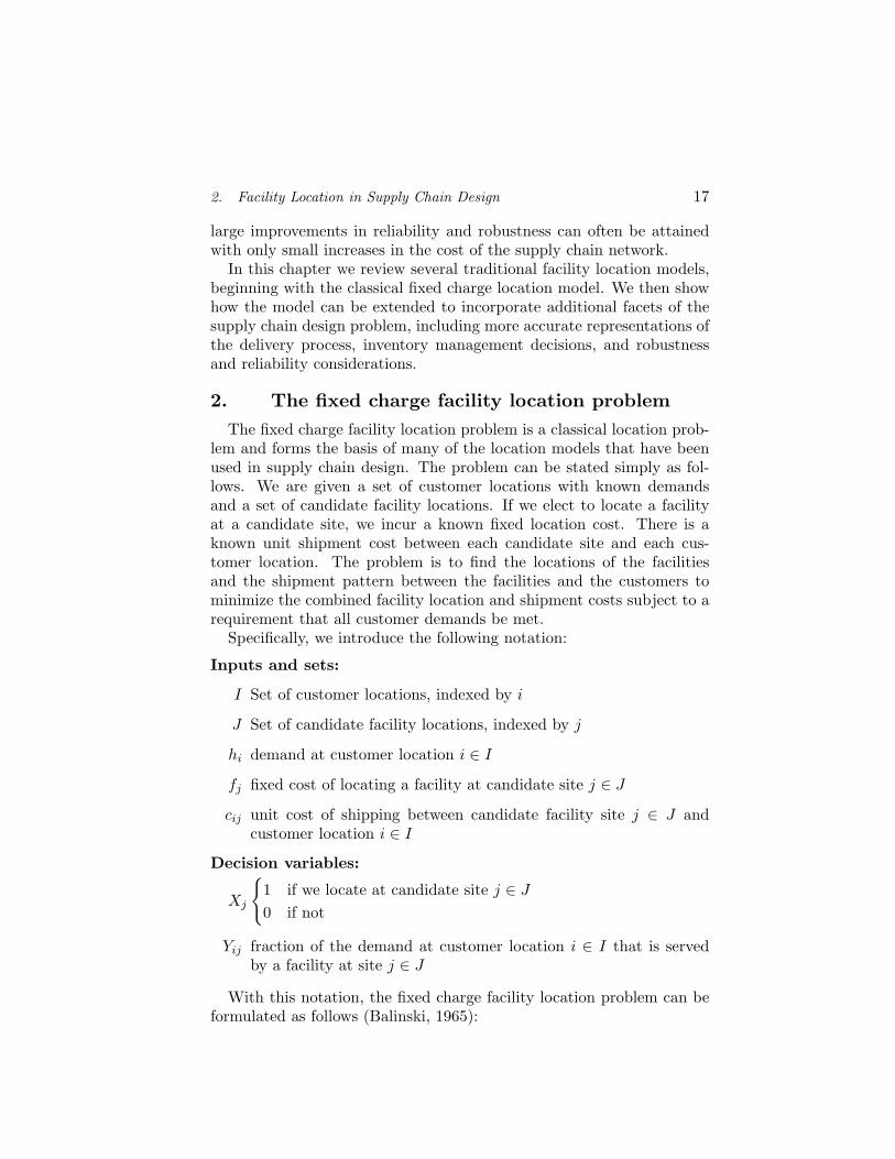
The fixed charge facility location problem is a classical location prob-lem and forms the basis of many of the location models that have beenused in supply chain design. The problem can be stated simply as fol-lows. We are given a set of customer locations with known demandsand a set of candidate facility locations. If we elect to locate a facilityat a candidate site, we incur a known fixed location cost. There is aknown unit shipment cost between each candidate site and each cus-tomer location. The problem is to find the locations of the facilitiesand the shipment pattern between the facilities and the customers tominimize the combined facility location and shipment costs subject to arequirement that all customer demands be met.

Specifically, we introduce the following notation:

Inputs and sets:

I Set of customer locations, indexed by i

J Set of candidate facility locations, indexed by j

hi demand at customer location i ∈ I

fj fixed cost of locating a facility at candidate site j ∈ J

cij unit cost of shipping between candidate facility site j ∈ J andcustomer location i ∈ I

Decision variables:

Xj

{

1 if we locate at candidate site j ∈ J

0 if not

Yij fraction of the demand at customer location i ∈ I that is servedby a facility at site j ∈ J

With this notation, the fixed charge facility location problem can beformulated as follows (Balinski, 1965):


Minimize∑

j∈J

fjXj +∑

j∈J

∑

i∈I

hicijY sij (2.1)

Subject to∑

j∈J

Yij = 1 ∀ i ∈ I (2.2)

Yij − Xj ≤ 0 ∀ i ∈ I; ∀ j ∈ J (2.3)

Xj ∈ {0, 1} ∀ j ∈ J (2.4)

Yij ≥ 0 ∀ i ∈ I; ∀ j ∈ J (2.5)

The objective function (2.1) minimizes the sum of the fixed facility lo-cation costs and the transportation or shipment costs. Constraint (2.2)stipulates that each demand node is fully assigned. Constraint (2.3)states that a demand node cannot be assigned to a facility unless weopen that facility. Constraint (2.4) is a standard integrality constraintand constraint (2.5) is a simple non-negativity constraint.

The formulation given above assumes that facilities have unlimitedcapacity; the problem is sometimes referred to as the uncapacitatedfixed charge location problem. It is well known that at least one optimalsolution to this problem involves assigning all of the demand at eachcustomer location i ∈ I fully to the nearest open facility site j ∈ J . Inother words, the assignment variables, Yij , will naturally take on integervalues in the solution to this problem. Many firms insist on or stronglyprefer such single sourcing solutions as they make the management ofthe supply chain considerably simpler. Capacitated versions of the fixedcharge location problem do not exhibit this property; enforcing singlesourcing is significantly more difficult in this case (as discussed below).

A number of solution approaches have been proposed for the uncapac-itated fixed charge location problem. Simple heuristics typically beginby constructing a feasible solution by greedily adding or dropping facil-ities from the solution until no further improvements can be obtained.Maranzana (1964) proposed a neighborhood search improvement algo-rithm for the closely related P -median problem (Hakimi (1964,1965))that exploits the ease in finding optimal solutions to 1-median problem:it partitions the customers by facility and then finds the optimal locationwithin each partition. If any facility changes, the algorithm repartitionsthe customers and continues until no improvement in the solution canbe found. Teitz and Bart (1968) proposed an exchange or “swap” al-gorithm for the P -median problem that can also be extended to thefixed charge facility location problem. Hansen and Mladenovic (1997)proposed a variable neighborhood search algorithm for the P -medianproblem that can also be used for the fixed charge location problem.Clearly, improvement heuristics designed for the P -median problem will


not perform well for the fixed charge location problem if the startingnumber of facilities is sub-optimal. One way of resolving this limitationis to apply more sophisticated heuristics to the problem. Al-Sultan andAl-Fawzan (1999) applied tabu search (Glover (1989,1990); Glover andLaguna (1997)) to the uncapacitated fixed charge location problem. Thealgorithm was tested successfully on small- to moderate-sized problems.

Erlenkotter (1978) proposed the well-known DUALOC procedure tofind optimal solutions to the problem. Galvao (1993) and Daskin (1995)review the use of Lagrangian relaxation algorithms in solving the un-capacitated fixed charge location problem. When embedded in branchand bound, Lagrangian relaxation can be used to solve the fixed chargelocation problem optimally (Geoffrion (1974)). The reader interested ina more comprehensive review of the uncapacitated fixed charge locationproblem is referred to either Krarup and Pruzan (1983) or Cornuejols,Nemhauser and Wolsey (1990).

One natural extension of the problem is to consider capacitated facil-ities. If we let bj be the maximum demand that can be assigned to afacility at candidate site j ∈ J , formulation (2.1)–(2.5) can be extendedto incorporate facility capacities by including the following additionalconstraint:

∑

i∈I

hiYij − bjXj ≤ 0 ∀ j ∈ J (2.6)

Constraint (2.6) limits the total assigned demand at facility j ∈ J toa maximum of bj . From the perspective of the integer programmingproblem, this constraint obviates the need for constraint (2.3) since anysolution that satisfies (2.5) and (2.6) will also satisfy (2.3). However,the linear programming relaxation of (2.1)–(2.6) is often tighter if con-straint (2.3) is included in the problem.

For fixed values of the facility location variables, Xj , the optimalvalues of the assignment variables can be found by solving a traditionaltransportation problem. The embedded transportation problem is mosteasily recognized if we replace hiYij by Zij , the quantity shipped fromdistribution center j to customer i. The transportation problem for fixedfacility locations is then

Minimize∑

j∈J

∑

i∈I

cijZij (2.7)

subject to∑

j∈J

Zij = hi ∀ i ∈ I (2.8)

∑

i∈I

Zij ≤ bjXj ∀ j ∈ J (2.9)


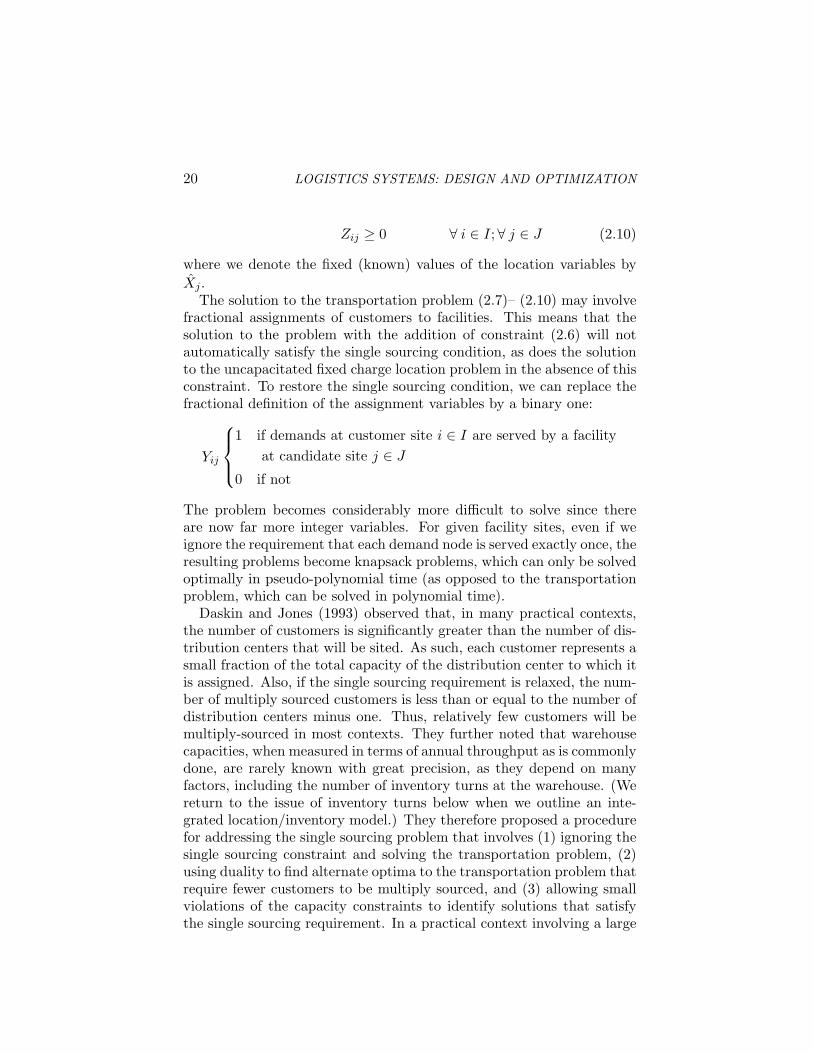
Zij ≥ 0 ∀ i ∈ I;∀ j ∈ J (2.10)

where we denote the fixed (known) values of the location variables by

Xj .The solution to the transportation problem (2.7)– (2.10) may involve

fractional assignments of customers to facilities. This means that thesolution to the problem with the addition of constraint (2.6) will notautomatically satisfy the single sourcing condition, as does the solutionto the uncapacitated fixed charge location problem in the absence of thisconstraint. To restore the single sourcing condition, we can replace thefractional definition of the assignment variables by a binary one:

Yij

1 if demands at customer site i ∈ I are served by a facility

at candidate site j ∈ J

0 if not

The problem becomes considerably more difficult to solve since thereare now far more integer variables. For given facility sites, even if weignore the requirement that each demand node is served exactly once, theresulting problems become knapsack problems, which can only be solvedoptimally in pseudo-polynomial time (as opposed to the transportationproblem, which can be solved in polynomial time).

Daskin and Jones (1993) observed that, in many practical contexts,the number of customers is significantly greater than the number of dis-tribution centers that will be sited. As such, each customer represents asmall fraction of the total capacity of the distribution center to which itis assigned. Also, if the single sourcing requirement is relaxed, the num-ber of multiply sourced customers is less than or equal to the number ofdistribution centers minus one. Thus, relatively few customers will bemultiply-sourced in most contexts. They further noted that warehousecapacities, when measured in terms of annual throughput as is commonlydone, are rarely known with great precision, as they depend on manyfactors, including the number of inventory turns at the warehouse. (Wereturn to the issue of inventory turns below when we outline an inte-grated location/inventory model.) They therefore proposed a procedurefor addressing the single sourcing problem that involves (1) ignoring thesingle sourcing constraint and solving the transportation problem, (2)using duality to find alternate optima to the transportation problem thatrequire fewer customers to be multiply sourced, and (3) allowing smallviolations of the capacity constraints to identify solutions that satisfythe single sourcing requirement. In a practical context involving a large


national retailer with over 300 stores and about a dozen distributioncenters, they found that this approach was perfectly satisfactory from amanagerial perspective.

In a classic paper, Geoffrion and Graves (1974) extend the traditionalfixed charge facility location problem to include shipments from plantsto distribution centers and multiple commodities. They introduce thefollowing additional notation:

Inputs and sets:

K Set of plant locations, indexed by k

L Set of commodities, indexed by l

Dli demand for commodity l ∈ L at customer i ∈ I

Slk supply of commodity l ∈ L at plant k ∈ K

V j ,V j minimum and maximum annual throughput allowed at distri-bution center j ∈ J

vj variable unit cost of throughput at candidate site j ∈ J

clkji unit cost of producing and shipping commodity l ∈ L betweenplant k ∈ K, candidate facility site j ∈ J and customer locationi ∈ I

Decision variables:

Yij

1 if demands at customer site i ∈ I are served by a facility

at candidate site j ∈ J

0 if not

Zlkji quantity of commodity l ∈ L shipped between plant k ∈ K, can-didate facility site j ∈ J and customer location i ∈ I

With this notation, Geoffrion and Graves formulate the following ex-tension of the fixed charge facility location problem.

Minimize∑

j∈J

fjXj +∑

j∈J

vj

(

∑

l∈L

∑

i∈I

DliYij

)

+∑

l∈L

∑

k∈K

∑

j∈J

∑

i∈I

clkjiZlkji

(2.11)

subject to∑

i∈I

∑

j∈J

Zlkji ≤ Slk ∀ k ∈ K;∀ l ∈ L (2.12)

∑

k∈K

Zlkji = DliYij ∀ l ∈ L;∀ j ∈ J ;∀ i ∈ I

(2.13)


∑

j∈J

Yij = 1 ∀ i ∈ I (2.14)

V jXj ≤∑

i∈I

∑

l∈L

DliYij ≤ V jXj ∀ j ∈ J (2.15)

Xj ∈ {0, 1} ∀ j ∈ J (2.16)

Yij ∈ {0, 1} ∀ i ∈ I;∀ j ∈ J (2.17)

Zlkji ≥ 0 ∀ i ∈ I;∀ j ∈ J

∀ k ∈ K;∀ l ∈ L (2.18)

The objective function (2.11) minimizes the sum of the fixed distributioncenter (DC) location costs, the variable DC costs and the transporta-tion costs from the plants through the DCs to the customers. Con-straint (2.12) states that the total amount of commodity l ∈ L shippedfrom plant k ∈ K cannot exceed the capacity of the plant to producethat commodity. Constraint (2.13) says that the amount of commodityl ∈ L shipped to customer i ∈ I via DC j ∈ J must equal the amountof that commodity produced at all plants that is destined for that cus-tomer and shipped via that DC. This constraint stipulates that demandmust be satisfied at each customer node for each commodity and alsoserves as a linking constraint between the flow variables (Zlkji) and theassignment variables (Yij). Constraint (2.14) is the now-familiar single-sourcing constraint. Constraint (2.15) imposes lower and upper boundson the throughput processed at each distribution center that is used.This also serves as a linking constraint (e.g., it replaces constraint (2.3))between the location variables (Xj) and the customer assignment vari-ables (Yij). Alternatively, it can be thought of as an extension of thecapacity constraint (2.6) above.

In addition to the constraints above, Geoffrion and Graves allow forlinear constraints on the location and assignment variables. These caninclude constraints on the minimum and maximum number of distribu-tion centers to be opened, relationships between the feasible open DCs,more detailed capacity constraints if different commodities use differentamounts of a DC’s resources, and certain customer service constraints.The authors apply Benders decomposition (Benders (1962)) to the prob-lem after noting that, if the location and assignment variables are fixed,the remaining problem breaks down into |L| transportation problems,one for each commodity.

Geoffrion and Graves highlight eight different forms of analysis thatwere performed for a large food company using the model arguing, asdo Geoffrion and Powers (1980), that the value of a model such as


(2.11)–(2.18) extends far beyond the mere solution of a single instanceof the problem to include a range of sensitivity and what-if analyses.

3. Integrated location/routing models

An important limitation of the fixed charge location model, and eventhe multi-echelon, multi-commodity extension of Geoffrion and Graves,is the assumption that full truckload quantities are shipped from a dis-tribution center to a customer. In many contexts, shipments are made inless-than-truckload (LTL) quantities from a facility to customers alonga multiple-stop route. In the case of full truckload quantities, the costof delivery is independent of the other deliveries made, whereas in thecase of LTL quantities, the cost of delivery depends on the other cus-tomers on the route and the sequence in which customers are visited.Eilon, Watson-Gandy and Christofides (1971) were among the first tohighlight the error introduced by approximating LTL shipments by fulltruckloads. During the past three decades, a sizeable body of literaturehas developed on integrated location/routing models.

Integrated location/routing problems combine three components ofsupply chain design: facility location, customer allocation to facilitiesand vehicle routing. Many different location/routing problems have beendescribed in the literature, and they tend to be very difficult to solvesince they merge two NP-hard problems: facility location and vehiclerouting. Laporte (1988) reviews early work on location/routing prob-lems; he summarizes the different types of formulations, solution algo-rithms and computational results of work published prior to 1988. Morerecently, Min, Jayaraman, and Srivastava (1998) develop a hierarchicaltaxonomy and classification scheme that they use to review the existinglocation/routing literature. They categorize papers in terms of problemcharacteristics and solution methodology. One means of classification isthe number of layers of facilities. Typically, three-layer problems includeflows from plants to distribution centers to customers, while two-layerproblems focus on flows from distribution centers to customers.

An example of a three-layer location/routing problem is the formula-tion of Perl (1983) and Perl and Daskin (1985); their model extends themodel of Geoffrion and Graves to include multiple stop tours serving thecustomer nodes but it is limited to a single commodity. Perl defines thefollowing additional notation:

Inputs and sets:

P set of points = I ∪ J

dij distance between node i ∈ P and node j ∈ P


vj variable cost per unit processed by a facility at candidate facilitysite j ∈ J

tj maximum throughput for a facility at candidate facility site j ∈ J

S set of supply points (analogous to plants in the Geoffrion andGraves model), indexed by s

csj unit cost of shipping from supply point s ∈ S to candidate facilitysite j ∈ J

K set of candidate vehicles, indexed by k

σk capacity of vehicle k ∈ K

τk maximum allowable length of a route served by vehicle k ∈ K

αk cost per unit distance for delivery on route k ∈ K

Decision variables:

Zijk

{

1 if vehicle k ∈ K goes directly from point i ∈ P to point j ∈ P

0 if not

Wsj quantity shipped from supply source s ∈ S to facility site j ∈ J

With this notation (and the notation defined previously), Perl (1983)formulates the following integrated location/routing problem:

Minimize∑

j∈J

fjXj +∑

s∈S

{

∑

j∈J

csjWsj

}

+∑

j∈J

vj

{

∑

i∈I

hiYij

}

+∑

k∈K

αk

{

∑

j∈P

∑

i∈P

dijZijk

}

(2.19)

Subject to:∑

k∈K

∑

j∈P

Zijk = 1 ∀ i ∈ I (2.20)

∑

i∈I

hi

{

∑

j∈P

Zijk

}

≤ σk ∀ k ∈ K (2.21)

∑

j∈P

∑

i∈P

dijZijk ≤ τk ∀ k ∈ K (2.22)

∑

i∈V

∑

j∈V

∑

k∈K

Zijk ≥ 1 ∀ subsets V ⊂ P

such that J ⊂ V (2.23)


∑

j∈P

Zijk −∑

j∈P

Zjik = 0 ∀ i ∈ P ;∀ k ∈ K (2.24)

∑

j∈J

∑

i∈I

Zijk ≤ 1 ∀ k ∈ K (2.25)

∑

s∈S

Wsj −∑

i∈I

hiYij = 0 ∀ j ∈ J (2.26)

∑

s∈S

Wsj − tjXj ≤ 0 ∀ j ∈ J (2.27)

∑

m∈P

Zimk +∑

h∈P

Zjhk − Yij ≤ 1 ∀ j ∈ J ; ∀ i ∈ I; ∀ k ∈ K

(2.28)

Xj ∈ {0, 1} ∀ j ∈ J (2.29)

Yij ∈ {0, 1t} ∀ i ∈ I; ∀ j ∈ J (2.30)

Zijk ∈ {0, 1} ∀ i ∈ P ;∀ j ∈ P ;∀ k ∈ K

(2.31)

Wsj ≥ 0 ∀ s ∈ S; ∀ j ∈ J (2.32)

The objective function (2.19) minimizes the sum of the fixed facility lo-cation costs, the shipment costs from the supply points (plants) to the fa-cilities, the variable facility throughput costs and the routing costs to thecustomers. Constraint (2.20) requires each customer to be on exactly oneroute. Constraint (2.21) imposes a capacity restriction for each vehicle,while constraint (2.22) limits the length of each route. Constraint (2.23)requires each route to be connected to a facility. The constraint requiresthat there be at least one route that goes from any set V (a proper sub-set of the points P that contains the set of candidate facility sites) to itscomplement, thereby precluding routes that only visit customer nodes.Constraint (2.24) states that any route entering node i ∈ P also mustexit that same node. Constraint (2.25) states that a route can operateout of only one facility. Constraint (2.26) defines the flow into a facilityfrom the supply points in terms of the total demand that is served by thefacility. Constraint (2.27) restricts the throughput at each facility to themaximum allowed at that site and links the flow variables and the facilitylocation variables. Thus, if a facility is not opened, there can be no flowthrough the facility, which in turn (by constraint (2.26)) precludes anycustomers from being assigned to the facility. Constraint (2.28) statesthat if route k ∈ K leaves customer node i ∈ I and also leaves facilityj ∈ J , then customer i ∈ I must be assigned to facility j ∈ J . Thisconstraint links the vehicle routing variables (Zijk) and the assignment


variables (Yij). Constraints (2.29)–(2.32) are standard integrality andnon-negativity constraints.

Even for small problem instances, the formulation above is a difficultmixed integer linear programming problem. Perl solves the problem us-ing a three-phased heuristic. The first phase finds minimum cost routes.The second phase determines which facilities to open and how to al-locate the routes from phase one to the selected facilities. The thirdphase attempts to improve the solution by moving customers betweenfacilities and re-solving the routing problem with the set of open facili-ties fixed. The algorithm iterates between the second and third phasesuntil the improvement at any iteration is less than some specified value.Wu, Low, and Bai (2002) propose a similar two-phase heuristic for theproblem and test it on problems with up to 150 nodes.

Like the three-layer formulation of Perl, two-layer location/routingformulations (e.g., Laporte, Nobert and Pelletier (1983), Laporte, Nobertand Arpin (1986) and Laporte, Nobert and Taillefer (1988)) usually arebased on integer linear programming formulations for the vehicle rout-ing problem (VRP). Flow formulations of the VRP often are classifiedaccording to the number of indices of the flow variable: Xij = 1 ifa vehicle uses arc (i, j) or Xijk = 1 if vehicle k uses arc (i, j). Thesize and structure of these formulations make them difficult to solve us-ing standard integer programming or network optimization techniques.Motivated by the successful implementation of exact algorithms for set-partitioning-based routing models, Berger (1997) formulates a two-layerlocation/routing problem that closely resembles the classical fixed chargefacility location problem. Unlike other location/routing problems, sheformulates the routes in terms of paths, where a delivery vehicle may notbe required to return to the distribution center after the final deliveryis made. The model is appropriate in situations where the deliveries aremade by a contract carrier or where the commodities to be delivered areperishable. In the latter case, the time to return from the last customerto the distribution center is much less important than the time from thefacility to the last customer. Berger defines the following notation:

Inputs and sets:

Pj set of feasible paths from candidate distribution center j ∈ J

cjk cost of serving the path k ∈ Pj

ajik 1 if delivery path k ∈ Pj visits customer i ∈ I; 0 if not


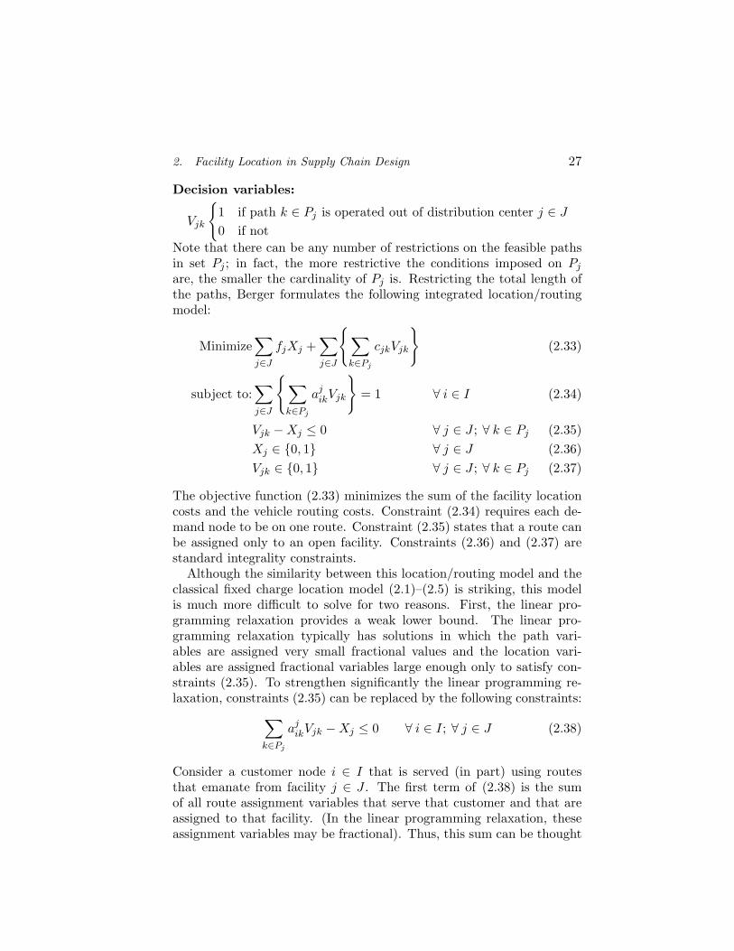
Decision variables:

Vjk

{

1 if path k ∈ Pj is operated out of distribution center j ∈ J

0 if not

Note that there can be any number of restrictions on the feasible pathsin set Pj ; in fact, the more restrictive the conditions imposed on Pj

are, the smaller the cardinality of Pj is. Restricting the total length ofthe paths, Berger formulates the following integrated location/routingmodel:

Minimize∑

j∈J

fjXj +∑

j∈J

{

∑

k∈Pj

cjkVjk

}

(2.33)

subject to:∑

j∈J

{

∑

k∈Pj

ajikVjk

}

= 1 ∀ i ∈ I (2.34)

Vjk − Xj ≤ 0 ∀ j ∈ J ; ∀ k ∈ Pj (2.35)

Xj ∈ {0, 1} ∀ j ∈ J (2.36)

Vjk ∈ {0, 1} ∀ j ∈ J ; ∀ k ∈ Pj (2.37)

The objective function (2.33) minimizes the sum of the facility locationcosts and the vehicle routing costs. Constraint (2.34) requires each de-mand node to be on one route. Constraint (2.35) states that a route canbe assigned only to an open facility. Constraints (2.36) and (2.37) arestandard integrality constraints.

Although the similarity between this location/routing model and theclassical fixed charge location model (2.1)–(2.5) is striking, this modelis much more difficult to solve for two reasons. First, the linear pro-gramming relaxation provides a weak lower bound. The linear pro-gramming relaxation typically has solutions in which the path vari-ables are assigned very small fractional values and the location vari-ables are assigned fractional variables large enough only to satisfy con-straints (2.35). To strengthen significantly the linear programming re-laxation, constraints (2.35) can be replaced by the following constraints:

∑

k∈Pj

ajikVjk − Xj ≤ 0 ∀ i ∈ I; ∀ j ∈ J (2.38)

Consider a customer node i ∈ I that is served (in part) using routesthat emanate from facility j ∈ J . The first term of (2.38) is the sumof all route assignment variables that serve that customer and that areassigned to that facility. (In the linear programming relaxation, theseassignment variables may be fractional). Thus, this sum can be thought


of as the fraction of demand node i ∈ I that is served out of facilityj ∈ J . The constraint requires the location variable to be no smallerthan the largest of these sums for customers assigned (in part) to routesemanating from the facility.

Second, there is an exponential number of feasible paths associatedwith any candidate facility, so complete enumeration of all possiblecolumns of the problem is prohibitive. Instead, Berger develops a branch-and-price algorithm, which uses column generation to solve the lin-ear programs at each node of the branch-and-bound tree. The pricingproblem for the model decomposes into a set of independent resource-constrained shortest path problems.

The development and the use of location/routing models have beenmore limited than both facility location and vehicle routing models. Inour view, the reason is that it is difficult to combine, in a meaningful way,facility location decisions, which typically are strategic and long-term,and vehicle routing decisions, which typically are tactical and short-term.The literature includes several papers that attempt to accommodate thefact that the set of customers to be served on a route may change daily,while the location of a distribution center may remain fixed for years.One approach is to define a large number of customers and to intro-duce a probability that each customer will require service on any day.Jaillet (1985, 1988) introduces this concept in the context of the proba-bilistic traveling salesman problem. Jaillet and Odoni (1988) provide anoverview of this work and related probabilistic vehicle routing problems.The idea is extended to location/routing problems in Berman, Jailletand Simchi-Levi (1995). Including different customer scenarios, how-ever, increases the difficulty of the problem, so this literature tends tolocate a single distribution center. In our view, the problem of approxi-mating LTL vehicle tours in facility location problems without incurringthe cost of solving an embedded vehicle routing or traveling salesmanproblem remains an open challenge worthy of additional research.

4. Integrated location/inventory models

The fixed charge location problem ignores the inventory impacts offacility location decisions; it deals only with the tradeoff between facil-ity costs, which increase with the number of facilities, and the averagetravel cost, which decreases approximately as the square root of thenumber of facilities located (call it N). Inventory costs increase ap-proximately as the square root of N . As such, they introduce anotherforce that tends to drive down the optimal number of facilities to locate.Baumol and Wolfe (1958) recognized the contribution of inventory to


distribution costs over forty years ago when they stated, “standard in-ventory analysis suggests that, optimally, important inventory compo-nents will vary approximately as the square root of the number of ship-ments going through the warehouse”. (p. 255) If the total number ofshipments is fixed, the number through any warehouse is approximatelyequal to the total divided by N . According to Baumol and Wolfe, thecost at each warehouse is then proportional to the square root of thisquantity. When the cost per warehouse is multiplied by N , we see thatthe total distribution cost varies approximately with the square root ofN . This argument treats the cost of holding working or cycle stock;Eppen (1979) argued that safety stock costs also increase as the squareroot of N (assuming equal variance of demand at each customer andindependence of customer demands).

While the contribution of inventory to distribution costs has beenrecognized for many years, only recently have we been able to solve thenon-linear models that result from incorporating inventory decisions infacility location models. Shen (2000) and Shen, Coullard, and Daskin(2003) introduced a location model with risk pooling (LMRP). Themodel minimizes the sum of fixed facility location costs, direct trans-portation costs to the customers (which are assumed to be linear inthe quantity shipped), working and safety stock inventory costs at thedistribution centers and shipment costs from a plant to the distributioncenter (which may include a fixed cost per shipment). The last two quan-tities — the inventory costs at the distribution centers and the shipmentcosts of goods to the distribution centers — depend on the allocationof customers to the distribution centers. Shen introduces the followingadditional notation:

Inputs and sets:

µi, σ2

i mean and variance of the demand per unit time at customer i ∈ I

cij a term that captures the annualized unit cost of supplying cus-tomer i ∈ I from facility j ∈ J as well as the variable shippingcost from the supplier to facility j ∈ J

ρj a term that captures the fixed order costs at facility j ∈ J aswell as the fixed transport costs per shipment from the supplier tofacility j ∈ J and the working inventory carrying cost at facilityj ∈ J

ωj a term that captures the lead time of shipments from the supplierto facility j ∈ J as well as the safety stock holding cost

With this notation, Shen formulates the LMRP as follows:


Minimize∑

j∈J

fjXj +∑

j∈J

∑

i∈I

cijµiYij +∑

j∈J

ρj

√

∑

i∈I

µiYij

+∑

j∈J

ωj

√

∑

i∈I

σ2

i Yij (2.39)

subject to:∑

j∈J

Yij = 1 ∀ i ∈ I (2.2)

Yij − Xj ≤ 0 ∀ i ∈ I; ∀ j ∈ J (2.3)

Xj ∈ {0, 1} ∀ j ∈ J (2.4)

Yij ≥ 0 ∀ i ∈ I; ∀ j ∈ J (2.5)

The first term of the objective function (2.39) represents the fixed facil-ity location costs. The second term captures the cost of shipping fromthe facilities to the customers as well as the variable shipment costs fromthe supplier to the facilities. The third term represents the working in-ventory carrying costs which include any fixed (per shipment) costs ofshipping from the supplier to the facilities. The final term representsthe safety stock costs at the facilities. Note that the objective functionis identical to that of the fixed charge location problem (2.1) with theaddition of two non-linear terms, the first of which captures economiesof scale regarding fixed ordering and shipping costs and the second ofwhich captures the risk pooling associated with safety stocks. Also notethat the constraints of the LMRP are identical to those of the fixedcharge location problem.

Shen (2000) and Shen, Coullard, and Daskin (2003) recast this modelas a set covering problem where the sets contain customers to be servedby facility j ∈ J . As in Berger’s location/routing model, the numberof possible sets is exponentially large. Thus, they propose solving theproblem using column generation. The pricing problems are non-linearinteger programs, but their structure allows for a low-order polynomialsolution algorithm. Shen assumes that the variance of demand is pro-portional to the mean. If demands are Poisson, this assumption is exactand not an approximation. With this assumption, he is able to collapsethe final two terms in the objective function into one term. The resultingpricing problems can then be solved in O(|I| log |I|t) time for each can-didate facility and in O(|J ||I| log |I|t) time for all candidate facilities ateach iteration of the column generation algorithm. Shu, Teo, and Shen(2001) showed that the pricing problem with two square root terms (i.e.,without assuming that the variance-to-mean ratio is constant for all cus-tomers) can be solved in O(|I|2 log |I|) time. Daskin, Coullard, and Shen


(2003) developed a Lagrangian relaxation algorithm for this model andfound it to be slightly faster than the column generation method.

One of the important qualitative findings from Shen’s model is that, asinventory costs increase as a percentage of the total cost, the number offacilities located by the LMRP is significantly smaller than the numberthat would have been sited by the uncapacitated fixed charge locationmodel, which ignores the risk pooling effects of inventory management.Shen and Daskin (2003) have extended the model above to account forcustomer service considerations. As customer service increases in im-portance, the number of facilities used in the optimal solution grows,eventually approaching and even exceeding the number used in the un-capacitated fixed charge model.

Several joint location/inventory models appeared in the literatureprior to Shen’s work. Barahona and Jensen (1998) solve a locationproblem with a fixed cost for stocking a given product at a DC. Er-lebacher and Meller (2000) use various heuristic techniques to solve ajoint location-inventory problem with a highly non-linear objective func-tion. Teo, Ou, and Goh (2001) present a

√2-approximation algorithm for

the problem of choosing DCs to minimize location and inventory costs,ignoring transportation costs. Nozick and Turnquist (2001a, 2001b)present models that, like Shen’s model, incorporate inventory consid-erations into the fixed charge location problem; however, they assumethat inventory costs are linear, rather than concave, and DC-customerallocations are made based only on distance, not inventory.

Ozsen, Daskin, and Coullard (2003) have extended the LMRP to in-corporate capacities at the facilities. Capacities are modeled in terms ofthe maximum (plausible) inventory accumulation during a cycle betweenorder receipts. This model is considerably harder to solve than is its un-capacitated cousin. However, it highlights an important new dimensionin supply chain operations that is not captured by the traditional capac-itated fixed charge location model. In the traditional model, capacityis typically measured in terms of throughput per unit time. However,this value can change as the number of inventory turns per unit timechanges. Thus, the measure of capacity in the traditional model is oftensuspect. Also, using the traditional model, there are only two ways todeal with capacity constraints as demand increases: build more facilitiesor reallocate customers to more remote facilities that have excess capac-ity. In the capacitated version of the LMRP, a third option is available,namely ordering more frequently in smaller quantities. By incorporat-ing this extra dimension of choice, the capacitated LMRP is more likelyto reflect actual managerial options than is the traditional fixed chargelocation model.


To some extent, merging inventory management with facility locationdecisions suffers from the same conceptual problems as merging vehi-cle routing with location. Inventory decisions, as argued above, can berevised much more frequently than can facility location decisions. Nev-ertheless, there are three important reasons for research to continue inthe area of integrated inventory-location modeling. First, early resultssuggest that the location decisions that are made when inventory is con-sidered can be radically different from those that would be made by aprocedure that fails to account for inventory. Second, as indicated above,the capacitated LMRP better models actual facility capacities than doesthe traditional fixed charge location model, as it introduces the optionof ordering more often to accommodate increases in demand. Third,we can solve fairly large instances of the integrated location-inventorymodel outlined above. In particular, the Lagrangian approach can oftensolve problems with 600 customers and 600 candidate facility sites in amatter of minutes on today’s desktop computers.

5. Planning under uncertainty

Long-term strategic decisions like those involving facility locations arealways made in an uncertain environment. During the time when de-sign decisions are in effect, costs and demands may change drastically.However, classical facility location models like the fixed charge locationproblem treat data as though they were known and deterministic, eventhough ignoring data uncertainty can result in highly sub-optimal solu-tions. In this section, we discuss approaches to facility location underuncertainty that have appeared in the literature.

Most approaches to decision making under uncertainty fall into oneof two categories: stochastic programming or robust optimization. Instochastic programming, the uncertain parameters are described by dis-crete scenarios, each with a given probability of occurrence; the objec-tive is to minimize the expected cost. In robust optimization, parametersmay be described either by discrete scenarios or by continuous ranges; noprobability information is known, however, and the objective is typicallyto minimize the worst-case cost or regret. (The regret of a solution undera given scenario is the difference between the objective function value ofthe solution under the scenario and the optimal objective function valuefor that scenario.) Both approaches seek solutions that perform well,though not necessarily optimally, under any realization of the data. Weprovide a brief overview of the literature on facility location under un-certainty here. For a more comprehensive review, the reader is referredto Owen and Daskin (1998) or Berman and Krass (2001).


Sheppard (1974) was one of the first authors to propose a stochasticapproach to facility location. He suggests selecting facility locations tominimize the expected cost, though he does not discuss the issue atlength. Weaver and Church (1983) and Mirchandani, Oudjit, and Wong(1985) present a multi-scenario version of the P -median problem. Theirmodel can be translated into the context of the fixed-charge locationproblem as follows. Let S be a set of scenarios. Each scenario s ∈ S has aprobability qs of occurring and specifies a realization of random demands(his) and travel costs (cijs). Location decisions must be made now,before it is known which scenario will occur. However, customers maybe assigned to facilities after the scenario is known, so the Y variablesare now indexed by a third subscript, s. The objective is to minimizethe total expected cost. The stochastic fixed charge location problem isformulated as follows:

Minimize∑

j∈J

fjXj +∑

s∈S

∑

j∈J

∑

i∈I

qshiscijsYijs (2.40)

subject to:∑

j∈J

Yijs = 1 ∀ i ∈ I; ∀ s ∈ S (2.41)

Yijs − Xj ≤ 0 ∀ i ∈ I; ∀ j ∈ J ; ∀ s ∈ S (2.42)

Xj ∈ {0, 1} ∀ j ∈ J (2.43)

Yijs ≥ 0 ∀ i ∈ I; ∀ j ∈ J ; ∀ s ∈ S (2.44)

The objective function (2.40) computes the total fixed cost plus theexpected transportation cost. Constraint (2.41) requires each customerto be assigned to a facility in each scenario. Constraint (2.42) requiresthat facility to be open. Constraints (2.43) and (2.44) are integralityand non-negativity constraints. The key to solving this model and theP -median-based models formulated by Weaver and Church (1983) andMirchandani, Oudjit, and Wong (1985) is recognizing that the problemcan be treated as a deterministic problem with |I||S| customers insteadof |I|.

Snyder, Daskin, and Teo (2003) consider a stochastic version of theLMRP. Other stochastic facility location models include those of Lou-veaux (1986), Franca and Luna (1982), Berman and LeBlanc (1984),Carson and Batta (1990), and Jornsten and Bjorndal (1994).

Robust facility location problems tend to be more difficult computa-tionally than stochastic problems because of their minimax structure.As a result, the literature on robust facility location generally fallsinto one of two categories: analytical results and polynomial-time al-gorithms for restricted problems like 1-median problems or P -medianson tree networks (see Chen and Lin (1998), Burkhard and Dollani (2001),


Vairaktarakis and Kouvelis (1999), and Averbakh and Berman (2000))and heuristics for more general problems (Serra, Ratick, and ReVelle(1996), Serra and Marianov (1998), and Current, Ratick, and ReVelle(1997)).

Solutions to the stochastic fixed charge problem formulated abovemay perform well in the long run but poorly in certain scenarios. Toaddress this problem, Snyder and Daskin (2003b) combine the stochasticand robust approaches by finding the minimum-expected-cost solutionto facility location problems subject to an additional constraint thatthe relative regret in each scenario is no more than a specified limit.They show empirically that by reducing this limit, one obtains solutionswith substantially reduced maximum regret without large increases inexpected cost. In other words, there are a number of near-optimal solu-tions to the fixed charge problem, many of which are much more robustthan the true optimal solution.

6. Location models with facility failures

Once a set of facilities has been built, one or more of them mayfrom time to time become unavailable — for example, due to inclementweather, labor actions, natural disasters, or changes in ownership. Thesefacility “failures” may result in excessive transportation costs as cus-tomers previously served by these facilities must now be served by moredistant ones. In this section, we discuss models for choosing facility lo-cations to minimize fixed and transportation costs while also hedgingagainst failures within the system. We call the ability of a system toperform well even when parts of the system have failed the “reliability”of the system. The goal, then, is to choose facility locations that areboth inexpensive and reliable.

The robust facility location models discussed in the previous sectionhedge against uncertainty in the problem data. By contrast, reliabilitymodels hedge against uncertainty in the solution itself. Another wayto view the distinction in the context of supply chain design is thatrobustness is concerned with “demand-side” uncertainty (uncertainty indemands, costs, or other parameters), while reliability is concerned with“supply-side” uncertainty (uncertainty in the availability of plants ordistribution centers).

The models discussed in this section are based on the fixed chargelocation problem; they address the tradeoff between operating cost (fixedlocation costs and day-to-day transportation cost—the classical fixedcharge problem objective) and failure cost (the transportation cost thatresults after a facility has failed). The first model considers the maximum


failure cost that can occur when a single facility fails, while the secondmodel considers the expected failure cost given a fixed probability offailure. The strategy behind both formulations is to assign each customerto a primary facility (which serves it under normal conditions) and oneor more backup facilities (which serve it when the primary facility hasfailed). Note that although we refer to primary and backup facilities,“primariness” is a characteristic of assignments, not facilities; that is, agiven facility may be a primary facility for one customer and a backupfacility for another.

In addition to the notation defined earlier, let

Yijk =

1 if facility j ∈ J serves as the primary facility and facility

k ∈ J serves as the secondary facility for customer i ∈ I

0 if not

and let V be a desired upper bound on the failure cost that may resultif a facility fails. Snyder (2003) formulates the maximum-failure-costreliability problem as follows:

Minimize∑

j∈J

fjXj +∑

i∈I

∑

j∈J

∑

k∈J

hicijYijk (2.45)

Subject to∑

j∈J

∑

k∈J

Yijk = 1 ∀ i ∈ I (2.46)

∑

k∈J

Yijk ≤ Xj ∀ i ∈ I;∀ j ∈ J (2.47)

Yijk ≤ Xk ∀ i ∈ I;∀ j ∈ J ;∀ k ∈ J (2.48)∑

i∈I

∑

k 6=J

k 6=j

∑

l∈J

hicikYikl+∑

i∈I

∑

k∈J

hicikYijk ≤ V ∀ j ∈ J

(2.49)

Yijj = 0 ∀ i ∈ I;∀ j ∈ J (2.50)

Xj ∈ {0, 1} ∀ j ∈ J (2.51)

Yijk ≥ 0 ∀ i ∈ I;∀ j ∈ J ;∀ k ∈ J (2.52)

The objective function (2.45) sums the fixed cost and transportationcost to customers from their primary facilities. (The summation overk is necessary to determine the assignments, but the objective functiondoes not depend on the backup assignments.) Constraint (2.46) requireseach customer to be assigned to one primary and one backup facility.Constraints (2.47) and (2.48) prevent a customer from being assigned toa primary or a backup facility, respectively, that has not been opened.


(The summation on the left-hand side of (2.47) can be replaced by Yijk

without affecting the IP solution, but doing so considerably weakens theLP bound.) Constraint (2.49) is the reliability constraint and requiresthe failure cost for facility j to be no greater than V . The first summationcomputes the cost of serving each customer from its primary facility ifits primary facility is not j, while the second summation computes thecost of serving customers assigned to j as their primary facility fromtheir backup facilities. Constraint (2.50) requires a customer’s primaryfacility to be different from its backup facility, and constraints (2.51)and (2.52) are standard integrality and non-negativity constraints. Thismodel can be solved for small instances using an off-the-shelf IP solver,but larger instances must be solved heuristically.

The expected-failure-cost reliability model (Snyder and Daskin, 2003a)assumes that multiple facilities may fail simultaneously, each with agiven probability q of failing. In this case, a single backup facility isinsufficient, since a customer’s primary and backup facilities may bothfail. Therefore, we define

Yijr =

1 if facility j ∈ J serves as the level-r facility for

customer i ∈ I

0 if not

A “level-r” assignment is one for which there are r closer facilities thatare open. If r = 0, this is a primary assignment; otherwise it is abackup assignment. The objective is to minimize a weighted sum ofthe operating cost (the fixed charge location problem objective) and theexpected failure cost, given by

∑

i∈I

∑

j∈J

|J |−1∑

r=0

hicijqr(1 − q)Yijr.

Each customer i is served by its level-r facility (call it j) if the r closerfacilities have failed (this occurs with probability qr) and if j itself hasnot failed (this occurs with probability 1− q). The full model is omittedhere. This problem can be solved efficiently using Lagrangian relaxation.

Few firms would be willing to choose a facility location solution thatis, say, twice as expensive as the optimal solution to the fixed chargeproblem just to hedge against occasional disruptions to the supply chain.However, Snyder and Daskin (2003a) show empirically that it often costsvery little to “buy” reliability: like robustness, reliability can be im-proved substantially with only small increases in cost.


7. Conclusions and directions for future work

Facility locations decisions are critical to the efficient and effectiveoperation of a supply chain. Poorly placed plants and warehouses canresult in excessive costs and degraded service no matter how well inven-tory policies, transportation plans, and information sharing policies arerevised, updated, and optimized. At the heart of many supply chainfacility location models is the fixed charge location problem. As morefacilities are located, the facilities tend to be closer to customers result-ing in lower transport costs, but higher facility costs. The fixed chargefacility location problem finds the optimal balance between fixed facilitycosts and transportation costs. Three important extensions of the basicmodel consider (1) facility capacities and single sourcing requirements,(2) multiple echelons in the supply chain, and (3) multiple products.

The fixed charge location problem, as well as these extensions, as-sume that shipments from the warehouses or distribution centers to thecustomers or retailers are made in truckload quantities. In reality, distri-bution to customers is often performed using less-than-truckload routesthat visit multiple customers. This chapter reviewed two different ap-proaches to formulating integrated location/routing models. However, asindicated above, these approaches suffer from the fundamental problemthat facility locations are typically determined at a strategic level whilevehicle routes are optimized at the operational level. In other words,the set of customers and their demands may change daily resulting indaily route changes, while the facilities are likely to be fixed for years.We believe that additional research is needed to find improved ways ofapproximating the impact of less-than-truckload deliveries on facility lo-cation costs without embedding a vehicle routing problem (designed toserve one realization of customer demands) in the facility location model.

Incorporating inventory decisions in facility location models appearsto be critical for supply chain modeling. As early as 1958, researchersrecognized that inventory costs would tend to increase with the squareroot of the number of facilities used. Only recently, however, have non-linear models that approximate this relationship between inventory costsand location decisions been formulated and solved optimally. While webelieve that these models represent an important step forward in locationmodeling for supply chain problems, considerable additional research isneeded. In particular, researchers should attempt to incorporate moresophisticated inventory models, including multi-item inventory modelsand models that account for inventory accumulation at all echelons ofthe supply chain. Heuristic approaches to the multi-item problem haverecently been proposed by Balcik (2003) and an optimal approach has


been suggested by Snyder (2003). The latter model, however, assumesthat items are ordered separately, resulting in individual fixed order costsfor each commodity purchased.

Finally, since facility location decisions are inherently strategic andlong-term in nature, supply chain location models must account for theinherent uncertainty surrounding future conditions. We have reviewed anumber of scenario-based location models as well as models that accountfor unreliability in the facilities themselves. This too is an area worthyof considerable additional research. For example, generating scenariosthat capture future uncertainty and the relationships between uncertainparameters is one critical area of research. Reliability-based locationmodels for supply chain management are still in their infancy. In fact, itis not immediately clear how to marry reliability modeling approachesand the integrated location/inventory models we reviewed, since the non-linearities introduced by the inventory terms complicate the computationof failure costs. In this regard, the more general techniques of stochasticprogramming (Birge and Louveaux, 1997) may ultimately prove fruitful.

References

Al-Sultan, K.S. and Al-Fawzan, M.A. (1999). A tabu search approachto the uncapacitated facility location problem. Annals of OperationsResearch, 86:91–103.

Averbakh, I. and Berman, O. (2000). Minmax regret median locationon a network under uncertainty. INFORMS Journal on Computing,12(2):104–110.

Balcik, B. (2003). Multi-Item Integrated Location/Inventory Problem.M.S. Thesis, Department of Industrial Engineering, Middle East Tech-nical University.

Balinski, M.L. (1965). Integer programming: Methods, uses, computa-tion. Management Science, 12:253–313.

Barahona, F. and Jensen, D. (1998). Plant Location with Minimum In-ventory. Mathematical Programming, 83:101–111.

Baumol, W.J. and Wolfe, P. (1958). A warehouse-location problem. Op-erations Research, 6:252–263.

Benders, J.F. (1962). Partitioning procedures for solving mixed-variablesprogramming problems. Numerische Mathematik, 4:238–252.

Berger, R. (1997), Location-Routing Models for Distribution System De-sign. Ph.D. Dissertation, Department of Industrial Engineering andManagement Sciences, Northwestern University, Evanston, IL.

Berman, O. and LeBlanc, B. (1984) Location-relocation of mobile facil-ities on a stochastic network. Transportation Science, 18(4):315–330.


Berman, O., Jaillet, P., and Simchi-Levi, D. (1995). Location-routingproblems with uncertainty. In: Z. Drezner (ed.), Facility Location: ASurvey of Applications and Methods, Springer, New York.

Berman, O. and Krass, D. (2002). Facility location problems withstochastic demands and congestion. In: Z. Drezner and H.W. Hamacher(eds), Facility Location: Applications and Theory, pp. 331–373 Springer,New York.

Birge, J.R. and Louveaux, F. (1997). Introduction to Stochastic Pro-gramming. Springer, New York.

Burkhard, R.E. and Dollani, H. (2001). Robust location problems withpos/neg weights on a tree. Networks, 38(2):102–113.

Carson, Y.M. and Batta, Y. (1990). Locating an ambulance on theAmherst Campus of the State University of New York at Buffalo.Interfaces, 20(5):43–49.

Chen, B.T. and Lin, C.S. (1998). Minimax-regret robust 1-median loca-tion on a tree. Networks, 31:93–103.

Cornuejols, G., Nemhauser, G.L., and Wolsey, L.A. (1990). The Unca-pacitated Facility Location Problem. In: P.B. Mirchandani and R.L.Francis (eds), Discrete Location Theory, pp. 119–171, Wiley, NewYork.

Current, J., Ratick, S., and ReVelle, C. (1997) Dynamic facility locationwhen the total number of facilities is uncertain: A decision analysisapproach. European Journal of Operational Research, 110(3):597–609.

Daskin, M.S. (1995), Network and Discrete Location: Models, Algorithmsand Applications. John Wiley and Sons, Inc., New York.

Daskin, M.S., Coullard, C., and Shen, Z.-J.M. (2002). An inventory-location model: Formulation, solution algorithm and computationalresults. Annals of Operations Research, 110:83–106.

Daskin, M.S. and Jones, P.C. (1993). A new approach to solving appliedlocation/allocation problems. Microcomputers in Civil Engineering,8:409–421.

Eilon, S., Watson-Gandy, C.D.T., and Christofides, N. (1971). Distri-bution Management: Mathematical Modeling and Practical Analysis.Hafner Publishing Co., NY.

Eppen, G. (1979). Effects of centralization on expected costs in a multi-location newsboy problem. Management Science, 25(5):498–501.

Erlebacher, S.J. and Meller, R.D. (2000). The interaction of location andinventory in designing distribution systems. IIE Transactions, 32:155–166.

Erlenkotter, D. (1978). A dual-based procedure for uncapacitated facilitylocation. Operations Research, 26:992–1009.


Franca, P.M. and Luna, H.P.L. (1982). Solving stochastic transportation-location problems by generalized Benders decomposition. Transporta-tion Science, 16:113–126.

Galvao, R.D. (1993). The use of Lagrangean relaxation in the solutionof uncapacitated facility location problems. Location Science, 1(1):57–79.

Geoffrion, A.M. (1974). Lagrangian relaxation for integer programming.Mathematical Programming Study, 2:82–114.

Geoffrion, A.M. and Graves, G.W. (1974). Multicommodity distribu-tion system design by Benders decomposition. Management Science,20(5):822–844.

Geoffrion, A.M. and Powers, R.F. (1980). Facility location analysis isjust the beginning (if you do it right). Interfaces, 10(2):22–30.

Glover, F. (1989). Tabu search — Part I. ORSA Journal on Computing,1(3):190–206.

Glover, F. (1990). Tabu search — Part II. ORSA Journal on Computing,2(1):4–32.

Glover, F. and Laguna, M. (1997). Tabu Search. Kluwer Academic Pub-lishers, Boston, MA.

Hansen, P. and Mladenovi, N. (1997). Variable neighborhood search forthe p-median. Location Science, 5(4):207–226.

Hakimi, S.L. (1964). Optimum location of switching centers and theabsolute centers and medians of a graph. Operations Research, 12:450–459.

Hakimi, S.L. (1965). Optimum distribution of switching centers in acommunication network and some related graph theoretic problems.Operations Research, 13:462–475.

Jaillet, P. (1985). The probabilistic traveling salesman problem. Tech-nical Report 185, Operations Research Center, M.I.T., Cambridge,MA.

Jaillet, P. (1988). A priori solution of a traveling salesman problem inwhich a random subset of the customers are visited. Operations Re-search, 36:929–936.

Jaillet, P. and Odoni, A. (1988). Probabilistic Vehicle Routing Problems.In: B.L. Golden and A.A. Assad (eds), Vehicle Routing: Methods andStudies, pp. 293–318, North-Holland, Amsterdam.

Jornsten, K. and Bjorndal, M. (1994) Dynamic location under uncer-tainty. Studies in Regional and Urban Planning, 3:163–184.

Krarup, J. and Pruzan, P.M. (1983). The simple plant location prob-lem: Survey and synthesis. European Journal of Operational Research,12:36–81.


Laporte, G. (1988). Location Routing Problems. In: B.L. Golden andA.A. Assad (eds), Vehicle Routing: Methods and Studies, pp. 163–197,North-Holland, Amsterdam.

Laporte, G., Nobert, Y., and Arpin, D. (1986). An exact algorithm forsolving a capacitated location-routing problem. Annals of OperationsResearch, 6:293–310.

Laporte, G., Nobert, Y., and Pelletier, J. (1983). Hamiltonian locationproblems. European Journal of Operational Research, 12:82–89.

Laporte G., Nobert, Y., and Taillefer, S. (1988). Solving a family ofmulti-depot vehicle routing and location-routing problems. Trans-portation Science, 22:161–172.

Louveaux, F.V. (1986). Discrete Stochastic Location Models. Annals ofOperations Research, 6:23–34.

Maranzana, F.E. (1964). On the location of supply points to minimizetransport costs. Operational Research Quarterly, 15:261–270.

Min, H., Jayaraman, V., and Srivastava, R. (1998). Combined location-routing problems: A synthesis and future research directions. Euro-pean Journal of Operational Research, 108:1–15.

Mirchandani, P.B., Oudjit, A., and Wong, R.T. (1985). Multidimensionalextensions and a nested dual approach for the m-median problem.European Journal of Operational Research, 21:121–137.

Nozick, L.K. and Turnquist, M.A. (2001a). Inventory, transportation,service quality and the location of distribution centers. European Jour-nal of Operational Research, 129:362–371.

Nozick, L.K. and Turnquist, M.A. (2001b). A two-echelon inventory al-location and distribution center location analysis. Transportation Re-search Part E, 37:421–441.

Owen, S.H. and Daskin, M.S. (1998). Strategic facility location: A re-view. European Journal of Operational Research, 111:423–447.

Ozsen, L., Daskin, M.S., and Coullard, C.R. (2003). Capacitated facilitylocation model with risk pooling. Submitted for publication.

Perl, J. (1983). A Unified Warehouse Location-Routing Analysis. Ph.D.Dissertation, Department of Civil Engineering, Northwestern Univer-sity, Evanston, IL.

Perl, J. and Daskin, M.S. (1985). A warehouse location-routing problem.Transportation Research, 19B(5):381–396.

Serra, D. and Marianov, V. (1998). The p-median problem in a changingnetwork: The case of Barcelona. Location Science, 6:383–394.

Serra, D., Ratick, S., and ReVelle, C. (1996). The maximum captureproblem with uncertainty. Environment and Planning B, 23:49–59.


Shen, Z.J. (2000). Efficient Algorithms for Various Supply Chain Prob-lems. Ph.D. Dissertation, Department of Industrial Engineering andManagement Sciences, Northwestern University, Evanston, IL 60208.

Shen, Z.-J.M., Coullard, C., and Daskin, M.S. (2003). A joint location-inventory model. Transportation Science, 37(1):40–55.

Shen, Z.-J.M. and Daskin, M.S. (2003). Tradeoffs between customer ser-vice and cost in an integrated supply chain design framework. Sub-mitted to Manufacturing and Service Operations Management.

Sheppard, E.S. (1974). A Conceptual Framework for Dynamic Location-Allocation Analysis. Environment and Planning A, 6:547–564.

Shu, J., Teo, C.-P., and Shen, Z.-J.M. (2001). Stochastic transportation-inventory network design. Preprint.

Simchi-Levi, D., Kaminsky, P., and Simchi-Levi, E. (2003). Designingand Managing the Supply Chain: Concepts Strategies and Case Stud-ies. Second Edition, McGraw-Hill, Irwin, Boston, MA.

Snyder, L.V. (2003). Supply Chain Robustness and Reliability: Modelsand Algorithms. Ph.D. Dissertation, Department of Industrial Engi-neering and Management Sciences, Northwestern University, Evanston,IL 60208.

Snyder, L.V. and Daskin, M.S. (2003a). Reliability models for facilitylocation: The expected failure cost case. Submitted for publication.

Snyder, L.V. and Daskin, M.S. (2003b). Stochastic p-robust locationproblems. Working Paper.

Snyder, L.V., Daskin, M.S., and Teo, C.-P. (2003). The stochastic loca-tion model with risk pooling. Submitted for publication.

Teitz, M.B. and Bart, P. (1968). Heuristic methods for estimating thegeneralized vertex median of a weighted graph. Operations Research,16:955–961.

Teo, C.-P., Ou, J., and Goh, M. (2001). Impact on inventory costs withconsolidation of distribution centers. IIE Transactions, 33(2):99–110.

Vairaktarakis, G.L. and Kouvelis, P. (1999),. Incorporation dynamic as-pects and uncertainty in 1-median location problems. Naval ResearchLogistics, 46(2):147–168.

Weaver, J.R. and Church, R.L. (1983). Computational procedures forlocation problems on stochastic networks. Transportation Science, 17:168–180.

Wu, T.-H., Low, C., and Bai, J.-W. (2002). Heuristic solutions to multi-depot location-routing problems. Computers and Operations Research,29:1393–1415.

chapter 2 · rosemary t. berger abstract in this chapter we outline the importance of facility...

Documents