chapter 2 risk and return: part i€¦ · in theory, investors should be concerned only with...

Solutions Manual for Intermediate Financial Management 12th Edition by

Eugene F. Brigham, Phillip R. Daves

Link full download: http://testbankcollection.com/download/intermediate-financial-

management-12th-edition-by-brigham-and-daves-solutions-manual/

Answers and Solutions: 2 - 1 © 2016 Cengage Learning. All Rights Reserved. May not be scanned, copied or duplicated, or posted to a publicly accessible website, in whole or in part.

Chapter 2

Risk and Return: Part I ANSWERS TO BEGINNING-OF-CHAPTER QUESTIONS

Our students have had an introductory finance course, and many have also taken a course on

investments and/or capital markets. Therefore, they have seen the Chapter 2 material previously.

However, we use the Beginning of Chapter (BOC) questions to review the chapter because our

students need a refresher.

With students who have not had as much background, it is best to go through the chapter on a

point-by-point basis, using the PowerPoint slides. With our students, this would involve

repeating too much of the intro course. Therefore, we just discuss the questions, including the

model for Question 6. Before the class, we tell our students that the chapter is a review and that

we will call on them to discuss the BOC questions in class. We expect students to be able to give

short, incomplete answers that demonstrate that they have read the chapter, and then we provide

more complete answers as necessary to make sure the key points are covered.

Our students have mainly taken multiple-choice exams, so they are uncomfortable with essay

tests. Also, we cover the chapters they were exposed to in the intro course rather quickly, so our

assignments often cover a lot of pages. We explain that much of the material is a review, and

that if they can answer the BOC questions (after the class discussion) they will do OK on the

exams. We also tell them, partly for motivation and partly to reduce anxiety, that our exams will

consist of 5 slightly modified BOC questions, of which they must answer 3. We also tell them

that they can use a 4-page “cheat sheet,” two sheets of paper, front and back. They can put

anything they want on it—formulas, definitions, outlines of answers to the questions, or

complete answers.

The better students write out answers to the questions before class, and then extend them after

class and before the exams. This helps them focus and get better prepared. Writing out answers

is a good way to study, and outlining answers to fit them on the cheat sheet (in really small font!)

also helps them learn. We try to get students to think in an integrated manner, relating topics

covered in different chapters to one another. Studying all of the BOC questions in a fairly

compressed period before the exams helps in this regard. They tell us that they learn a great deal

when preparing their cheat sheets.

We initially expected really excellent exams, given that the students had the questions and could

use cheat sheets. Some of the exams were indeed excellent, but we were surprised and

http://testbankcollection.com/download/intermediate-financial-management-12th-edition-by-brigham-and-daves-solutions-manual/



disappointed at the poor quality of many of the midterm exams. Part of the problem is that our

students were not used to taking essay exams. Also, they would have done better if they had

taken the exam after we covered cases (in the second half of the semester), where we apply the

text material to real-world cases. While both points are true, it’s also true that some students are

just better than others.

The students who received low exam grades often asked us what they did wrong. That’s often a

hard question to answer regarding an essay exam. What we ended up doing was make copies of

the best 2 or 3 student answers to each exam question, and then when students came in to see

why they did badly, we made them read the good answers before we talked with them. 95% of

the time, they told us they understand why their grade was low, and they resolved to do better

next time. Finally, since our students are all graduating seniors, we graded rather easily.

Answers

2-1 Stand-alone risk is the risk faced by an investor who holds just one asset, versus the risk

inherent in a diversified portfolio.

Stand-alone risk is measured by the standard deviation (SD) of expected returns or

the coefficient of variation (CV) of returns = SD/expected return.

A portfolio’s risk is measured by the SD of its returns, and the risk of the individual stocks in the

portfolio is measured by their beta coefficients. Note that unless returns on all stocks in a

portfolio are perfectly positively correlated, the portfolio’s SD will be less than the average

of the SD’s of the individual stocks. Diversification reduces risk.

In theory, investors should be concerned only with portfolio risk, but in practice many investors

are not well diversified, hence are concerned with stand-alone risk. Managers or other

employees who have large stockholdings in their companies are an example. They get

stock (or options) as incentive compensation or else because they founded the company,

and they are often constrained from selling to diversify. Note too that years ago brokerage

costs and administrative hassle kept people from diversifying, but today mutual funds

enable small investors to diversify efficiently. Also, the Enron and WorldCom debacles

and their devastating effects on 401k plans heavily in those stocks illustrated the

importance of diversification.

2-2 Diversification can eliminate unsystematic risk, but market risk will remain. See Figure 26 for

a picture of what happens as stocks are added to a portfolio. The graph shows that the risk

of the portfolio as measured by its SD declines as more and more stocks are added. This

is the situation if randomly selected stocks are added, but if stocks in the same industry are

added, the benefits of diversification will be lessened.

Conventional wisdom says that 40 to 50 stocks from a number of different industries is sufficient

to eliminate most unsystematic risk, but in recent years the markets have become

increasingly volatile, so now it takes somewhat more, perhaps 60 or 70. Of course, the






more stocks, the closer the portfolio will be to having zero unsystematic risk. Again, this

assumes that stocks are randomly selected. Note, however, that the more stocks the

portfolio contains, the greater the administrative costs. Mutual funds can help here.

Different diversified portfolios can have different amounts of risk. First, if the portfolio

concentrates on a given industry or sector (as sector mutual funds do), then the portfolio

will not be well diversified even if it contains 100 stocks. Second, the betas of the

individual stocks affect the risk of the portfolio. If the stock with the highest beta in each

industry is selected, then the portfolio may not have much unsystematic risk, but it will

have a high beta and thus have a lot of market risk. (Note: The market risk of a portfolio

is measured by the beta of the portfolio, and that beta is a weighted average of the

betas of the stocks in the portfolio.)

2-3 a. Note: This question is covered in more detail in Chapter 8, but students should remember

this material from their first finance course, so it is a review.

Expected: The rate of return someone expects to earn on a stock. It’s typically measured as D1/P0

+ g for a constant growth stock.

Required: The minimum rate of return that an investor must expect on a stock to induce him or

her to buy or hold the stock. It’s typically measured as rs = rrf + b(MRP), where MRP

is the market risk premium or the risk premium required for an average stock.

Historical: The average rate of return earned on a stock during some past period. The historical

return on an average large stock varied from –3% to +37% during the 1990s, and the

average annual return was about 15%. The worm turned after 1999—the average return

was negative in 2000, 2001, and 2002, with the S&P 500 down 23.4% in 2002. The

Nasdaq average of mostly tech stock did even worse, falling 31.5% in 2002 alone. Of

course, the bottom fell out of the market with the Global Economic Crisis in 2008 and

2009! The variations for individual stocks were much greater—the best performer on

the NYSE in 2000 gained 413% and the worst performer lost 100% of its value. Stocks

improved in the mid 2000s only to crash again in 2008 with the financial crisis. In short,

stock returns are highly variable!

b. Are the 3 types of return equal? 1) Expected = required?. The answer is, “maybe.” For the

market to be in equilibrium, the expected and required rate of return as seen by “the

marginal investor” must be equal for any given stock and therefore for the entire

market. If the expected return exceeded the required return, then investors would buy,

pushing the price up and the expected return down, and thus produce an equilibrium.

Note, though, that any individual investor may believe that a given stock’s expected

and required returns differ, so individuals may think there are bargains to be bought or

dogs to be sold. Also, new information is constantly hitting the market and changing

the opinions of marginal investors, and this leads to swings in the market. New




technology is causing new information to be disseminated ever more rapidly, and that

is leading to more rapid and violent market swings.

2) Historical = expected and/or required? There is no reason whatever to think that the historical

rate of return for any given year for either one stock or for all stocks on average will be

equal to the expected and/or required rate of return. Rational people don’t expect

abnormally good or bad performance to continue. On the other hand, people do argue

that investors expect to earn returns in the future that approximate average past returns.

For example, if stocks returned 9% on average in the past (from 1926 to 2013, which

is as far back as good data exist), then they may expect to earn about 9% on stocks in

the future. Note, though, that this is a controversial issue—the period 1926-2013 covers

a lot of very different economic environments, and investors may not expect the future

to replicate the past. Certainly investors didn’t expect future returns to equal distant

past returns during the height of the 1999 bull market or to lose money as they did in

2002 and 2008.

2-4 To be risk averse means to dislike risk. Most investors are risk averse. Therefore, if Securities

A and B both have an expected return of say 10%, but Security A has less risk than B, then

most investors will prefer A. As a result, A’s price will be bid up, and B’s price bid down,

and in the resulting equilibrium A’s expected rate of return will be below that of B. Of

course, A’s required rate of return will also be less than B’s, and in equilibrium the expected

and required returns will be equal.

One issue here is the type of risk investors are averse to—unsystematic, market, or both?

According to CAPM theory, only market risk as measured by beta is relevant and thus only

market risk requires a premium. However, empirical tests indicate that investors also

require a premium for bearing unsystematic risk as measured by the stock’s SD.

2-5 CAPM = Capital Asset Pricing Model. The CAPM establishes a metric for measuring the

market risk of a stock (beta), and it specifies the relationship between risk as measured by

beta and the required rate of return on a stock. Its principal developers (Sharpe and

Markowitz) won the Nobel Prize in 1990 for their work.

The key assumptions are spelled out in Chapter 3, but they include the following: (1) all investors

focus on a single holding period, (2) investors can lend or borrow unlimited amounts at the

risk-free rate, (3) there are no brokerage costs, and (4) there are no taxes. The assumptions

are not realistic, so the CAPM may be incorrect. Empirical tests have neither confirmed

nor refuted the CAPM with any degree of confidence, so it may or may not provide a valid

formula for measuring the required rate of return.

The SML, or Security Market Line, specifies the relationship between risk as measured by beta

and the required rate of return, rs = rrf + b(MRP). MRP = Expected rate of return on the

market – Risk-free rate = rm – rfr .






The data requirements are beta, the risk-free rate, and the rate of return expected on the market.

Betas are easy to get (by calculating them or from some source such as Value Line or

Yahoo!, but a beta shows how volatile a stock was in the past, not how volatile it will be in

the future. Therefore, historical betas may not reflect investors’ perceptions about a stock’s

future risk, which is what’s relevant. The risk-free rate is based on either T-bonds or T-

bills; these rates are easy to get, but it is not clear which should be used, and there can be a

big difference between bill and bond rates, depending on the shape of the yield curve.

Finally, it is difficult to determine the rate of return investors expect on an average stock.

Some argue that investors expect to earn the same average return in the future that they

earned in the past, hence use historical MRPs, but as noted above, that may not reflect

investors’ true expectations.

The bottom line is that we cannot be sure that the CAPM-derived estimate of the required rate of

return is actually correct.

2-6 a. Given historical returns on X, Y, and the Market, we could calculate betas for X and Y.

Then, given rrf and the MRP, we could use the SML equation to calculate X and Y’s

required rates of return. We could then compare these required returns with the given

expected returns to determine if X and Y are bargains, bad deals, or in equilibrium.

We assumed a set of data and then used an Excel model to calculate betas for X and Y, and the

SML required returns for these stocks. Note that in our Excel model (ch02M) we also

show, for the market, how to calculate the total return based on stock price changes plus

dividends. bx = 0.69; by = 1.66 and rx = 10.7%; ry = 14.6%. Since Y has the higher

beta, it has the higher required return.

In our examples, the returns all fall on the trend line. Thus, the two stocks have essentially no

diversifiable, unsystematic risk—all of their risk is market risk. If these were real

companies, they might have the indicated trend lines and betas, but the points would be

scattered about the trend line. See Figure 3-8 in Chapter 3, where data for General

Electric are plotted. Although the situation for our Stocks X and Y would never occur

for individual stocks, it would occur (approximately) for index funds, if Stock X were

an index fund that held stocks with betas that averaged 0.69 and Stock Y were an index

fund with b = 1.66 stocks.

b. Here we drop Year 1 and add Year 6, then calculate new betas and r’s. For Stock X, the beta

and required return would be reasonably stable. However, Y’s beta would fall, given

its sharp decline in a year when the market rose. In our Excel model, Y’s beta falls

from 1.66 to 0.19, and its required return as calculated with the SML falls to 8.8%.

The results for Y make little sense. The stock fell sharply because investors became worried

about its future prospects, which means that it fell because it became riskier. Yet its




beta fell. As a riskier stock, its required return should rise, yet the calculated return fell

from 14.6% to 8.8%, which is only a little above the riskless rate.

The problem is that Y’s low return tilted the regression line down—the point for Year 6 is in the

lower right quadrant of the Excel graph. The low R2 and the large standard error as

seen in the Excel regression make it clear that the beta, and thus the calculated required

return, are not to be trusted.

Note that in April 2001, the same month that PG&E declared bankruptcy, its beta as reported by

Finance.Yahoo was only 0.05, so our hypothetical Stock Y did what the real PG&E

actually did. The moral of the story is that the CAPM, like other cost of capital

estimating techniques, can be dangerous if used without care and judgment.

One final point on all this: The utilities are regulated, and regulators estimate their cost of capital

and use it as a basis for setting electric rates. If the estimated cost of capital is low, then

the companies are only allowed to earn a low rate of return on their invested capital. At

times, utilities like PG&E become more risky, have resulting low betas, and are then in

danger of having some squirrelly finance “expert” argue that they should be allowed to

earn an improper CAPM rate of return. In the industrial sector, a badly trained financial

analyst with a dumb supervisor could make the same mistake, estimate the cost of

capital to be below the true cost, and cause the company to make investments that

should not be made.

2-7 a. If technical trading rules could generate abnormal profits for an investor, then the market

would not even be weak form efficient. Finance researchers believe that markets are at

least weak form efficient because there are tens of thousands of analysts poring over

past returns, prices, volumes and other technical characteristics of stock prices, and if

any rules were consistently profitable, many of these analysts would discover this fact

and their trading would drive out the profitability of the strategy. In addition, most

studies find that technical trading rules do not generate abnormal profits. If technical

analysis does not generate abnormal profits, then the market is weak form efficient.

b. If fundamental analysis cannot generate abnormal profits, then the market is said to be semi-

strong form efficient.

c. If insider trading cannot generate abnormal profits, then the market is said to be strong form

efficient. Strong form efficiency means that the stock market’s prices impound all information

about the stock, no matter how well kept the secret is.

d. Internet chat rooms, close friends connected with the company and close friends not connected

with the company all provide non-public information. If a trader cannot make an abnormal

profit from trading on this information, then the market is strong form efficient. If a trader can

make abnormal profits from this information, then the market is not strong form efficient; it






may or may not be semi-strong form or weak form efficient, depending on whether abnormal

profits can be made from other strategies.

ANSWERS TO END-OF-CHAPTER QUESTIONS

2-1 a. Stand-alone risk is only a part of total risk and pertains to the risk an investor takes by

holding only one asset. Risk is the chance that some unfavorable event will occur. For

instance, the risk of an asset is essentially the chance that the asset’s cash flows will be

unfavorable or less than expected. A probability distribution is a listing, chart or graph

of all possible outcomes, such as expected rates of return, with a probability assigned

to each outcome. When in graph form, the tighter the probability distribution, the less

uncertain the outcome.

b. The expected rate of return (^r ) is the expected value of a probability distribution of

expected returns.

c. A continuous probability distribution contains an infinite number of outcomes and is

graphed from - and + .

d. The standard deviation (σ) is a statistical measure of the variability of a set of

observations. The variance (σ2) of the probability distribution is the sum of the squared

deviations about the expected value adjusted for deviation.

e. A risk averse investor dislikes risk and requires a higher rate of return as an inducement

to buy riskier securities. A realized return is the actual return an investor receives on

their investment. It can be quite different than their expected return.

f. A risk premium is the difference between the rate of return on a risk-free asset and the

expected return on Stock i which has higher risk. The market risk premium is the

difference between the expected return on the market and the risk-free rate.




g. CAPM is a model based upon the proposition that any stock’s required rate of return is

equal to the risk free rate of return plus a risk premium reflecting only the risk

remaining after diversification.

h. The expected return on a portfolio. r p, is simply the weighted-average expected return

of the individual stocks in the portfolio, with the weights being the fraction of total

portfolio value invested in each stock. The market portfolio is a portfolio consisting of

all stocks.

i. Correlation is the tendency of two variables to move together. A correlation coefficient

(ρ) of +1.0 means that the two variables move up and down in perfect synchronization,

while a coefficient of -1.0 means the variables always move in opposite directions. A

correlation coefficient of zero suggests that the two variables are not related to one

another; that is, they are independent.

j. Market risk is that part of a security’s total risk that cannot be eliminated by

diversification. It is measured by the beta coefficient. Diversifiable risk is also known

as company specific risk, that part of a security’s total risk associated with random

events not affecting the market as a whole. This risk can be eliminated by proper

diversification. The relevant risk of a stock is its contribution to the riskiness of a

welldiversified portfolio.

k. The beta coefficient is a measure of a stock’s market risk, A stock with a beta greater

than 1 has stock returns that tend to be higher than the market when the market is up

but tend to be below the market when the market is down. The opposite is true for a

stock with a beta less than 1..

l. The security market line (SML) represents in a graphical form, the relationship between

the risk of an asset as measured by its beta and the required rates of return for individual

securities. The SML equation is essentially the CAPM, ri = rRF + bi(RPM). It can also

be written in terms of the required market return: ri = rRF + bi(rM - rRF).

m. The slope of the SML equation is (rM - rRF), the market risk premium. The slope of the

SML reflects the degree of risk aversion in the economy. The greater the average

investors aversion to risk, then the steeper the slope, the higher the risk premium for all

stocks, and the higher the required return.

n. Equilibrium is the condition under which the expected return on a security is just equal






to its required return, r = r, and the market price is equal to the intrinsic value. The

Efficient Markets Hypothesis (EMH) states (1) that stocks are always in equilibrium

and (2) that it is impossible for an investor to consistently “beat the market.” In

essence, the theory holds that the price of a stock will adjust almost immediately in

response to any new developments. In other words, the EMH assumes that all

important information regarding a stock is reflected in the price of that stock. Financial

theorists generally define three forms of market efficiency: weak-form, semistrong-

form, and strong-form.

Weak-form efficiency assumes that all information contained in past price movements is

fully reflected in current market prices. Thus, information about recent trends in a

stock’s price is of no use in selecting a stock. Semistrong-form efficiency states that

current market prices reflect all publicly available information. Therefore, the only

way to gain abnormal returns on a stock is to possess inside information about the

company’s stock. Strong-form efficiency assumes that all information pertaining to a

stock, whether public or inside information, is reflected in current market prices. Thus,

no investors would be able to earn abnormal returns in the stock market.

o. The Fama-French 3-factor model has one factor for the excess market return (the

market return minus the risk free rate), a second factor for size (defined as the return

on a portfolio of small firms minus the return on a portfolio of big firms), and a third

factor for the book-to-market effect (defined as the return on a portfolio of firms with

a high book-to-market ratio minus the return on a portfolio of firms with a low bookto-

market ratio).

p. Most people don’t behave rationally in all aspects of their personal lives, and behavioral

finance assumes that investors have the same types of psychological behaviors in their

financial lives as in their personal lives.

Anchoring bias is the human tendency to “anchor” too closely on recent events when

predicting future events. Herding is the tendency of investors to follow the crowd.

When combined with overconfidence, anchoring and herding can contribute to market

bubbles.

2-2 a. The probability distribution for complete certainty is a vertical line.

b. The probability distribution for total uncertainty is the X axis from - to + .




2-3 Security A is less risky if held in a diversified portfolio because of its lower beta and negative

correlation with other stocks. In a single-asset portfolio, Security A would be more risky

because σA > σB and CVA > CVB.


2-4 The risk premium on a high beta stock would increase more.

RPj = Risk Premium for Stock j = (rM - rRF)bj.

If risk aversion increases, the slope of the SML will increase, and so will the market risk

premium (rM – rRF). The product (rM – rRF)bj is the risk premium of the jth stock. If bj is

low (say, 0.5), then the product will be small; RPj will increase by only half the increase in

RPM. However, if bj is large (say, 2.0), then its risk premium will rise by twice the increase

in RPM.

2-5 According to the Security Market Line (SML) equation, an increase in beta will increase a

company’s expected return by an amount equal to the market risk premium times the

change in beta. For example, assume that the risk-free rate is 6 percent, and the market risk

premium is 5 percent. If the company’s beta doubles from 0.8 to 1.6 its expected return

increases from 10 percent to 14 percent. Therefore, in general, a company’s expected

return will not double when its beta doubles.


SOLUTIONS TO END-OF-CHAPTER PROBLEMS

2-1 Investment Beta

$20,000 0.7

35,000 1.3

Total $55,000

($20,000/$55,000)(0.7) + ($35,000/$55,000)(1.3) = 1.08.

2-2 rRF = 4%; rM = 12%; b = 0.8; rs = ?

rs = rRF + (rM - rRF)b = 4%

+ (12% - 4%)0.8 =

10.4%.

2-3 rRF = 5%; RPM = 7%; rM = ?

rM = 5% + (7%)1 = 12% = rs when b = 1.0.

rs when b = 1.7 = ?

rs = 5% + 7%(1.7) = 16.9%.

2-4 Predicted return = ¯rRF,t + ai + bi(¯rM,t ¯rRF,t) + ci(¯rSMB,t) + di(¯rHML,t)

= 5% + 0.0% + 1.2(10% - 5%) + (-0.4)(3.2%) + 1.3(4.8%)

= 15.96%

2-5 r = (0.1)(-50%) + (0.2)(-5%) + (0.4)(16%) + (0.2)(25%) + (0.1)(60%)

= 11.40%.

σ2 = (-50% - 11.40%)2(0.1) + (-5% - 11.40%)2(0.2) + (16% - 11.40%)2(0.4)


+ (25% - 11.40%)2(0.2) + (60% - 11.40%)2(0.1) σ2

= 712.44; σ= 26.69%.

2-6 a. r m= (0.3)(15%) + (0.4)(9%) + (0.3)(18%) = 13.5%.

r j= (0.3)(20%) + (0.4)(5%) + (0.3)(12%) =

11.6%.

b. σM = [(0.3)(15% - 13.5%)2 + (0.4)(9% - 13.5%)2 + (0.3)(18% -13.5%)2]1/2

= 14.85% = 3.85%.

σJ = [(0.3)(20% - 11.6%)2 + (0.4)(5% - 11.6%)2 + (0.3)(12% - 11.6%)2]1/2

= 38.64% = 6.22%.

2-7 a. rA = rRF + (rM - rRF)bA

12% = 5% + (10% - 5%)bA

12% = 5% + 5%(bA)

7% = 5%(bA) 1.4

= bA.

b. rA = 5% + 5%(bA) rA

= 5% + 5%(2) rA =

15%.

2-8 a. ri = rRF + (rM - rRF)bi = 5% + (12% - 5%)1.4 = 14.8%.

b. 1. rRF increases to 6%:

rM increases by 1 percentage point, from 12% to 13%.

ri = rRF + (rM - rRF)bi = 6% + (12% - 5%)1.4 = 15.8%.


2. rRF decreases to 4%:

rM decreases by 1%, from 12% to 11%.

ri = rRF + (rM - rRF)bi = 4% + (12% - 5%)1.4 = 13.8%.

c. 1. rM increases to 14%:

ri = rRF + (rM - rRF)bi = 5% + (14% - 5%)1.4 = 17.6%.

2. rM decreases to 11%:

ri = rRF + (rM - rRF)bi = 5% + (11% - 5%)1.4 = 13.4%.


$70,000 $5,000

2-9 Old portfolio beta = (b) + (0.8)

$75,000 $75,000

1.2 = 0.9333b + 0.0533

1.1467 = 0.9333b

1.229 = b.

New portfolio beta = 0.9333(1.229) + 0.0667(1.6) = 1.25.

Alternative Solutions:

1. Old portfolio beta = 1.2 = (0.0667)b1 + (0.0667)b2 +...+ (0.0667)b20

1.2 = ( bi)(0.0667)

bi = 1.2/0.0667 = 18.0.

New portfolio beta = (18.0 - 0.8 + 1.6)(0.0667) = 1.253 = 1.25.

2. bi excluding the stock with the beta equal to 0.8 is 18.0 - 0.8 = 17.2, so the

beta of the portfolio excluding this stock is b = 17.2/14 = 1.2286. The beta of the new

portfolio is:

1.2286(0.9333) + 1.6(0.0667) = 1.1575 = 1.253.

$400,000 $600,000

2-10 Portfolio beta = (1.50) + (-0.50)

$4,000,000 $4,000,000

$1,000,000 $2,000,000

+ (1.25) + (0.75)

$4,000,000 $4,000,000

= 0.1)(1.5) + (0.15)(-0.50) + (0.25)(1.25) + (0.5)(0.75)

= 0.15 - 0.075 + 0.3125 + 0.375 = 0.7625.

rp = rRF + (rM - rRF)(bp) = 6% + (14% - 6%)(0.7625) = 12.1%.

Alternative solution: First compute the return for each stock using the CAPM equation

[rRF + (rM - rRF)b], and then compute the weighted average of these returns.


rRF = 6% and rM - rRF = 8%.

Stock Investment Beta r = rRF + (rM - rRF)b Weight

A $ 400,000 1.50 18% 0.10

B 600,000 (0.50) 2 0.15

C 1,000,000 1.25 16 0.25

D 2,000,000 0.75 12 0.50

Total $4,000,000 1.00

rp = 18%(0.10) + 2%(0.15) + 16%(0.25) + 12%(0.50) = 12.1%.

2-11 First, calculate the beta of what remains after selling the stock:

bp = 1.1 = ($100,000/$2,000,000)0.9 + ($1,900,000/$2,000,000)bR

1.1 = 0.045 + (0.95)bR

bR = 1.1105.

bN = (0.95)1.1105 + (0.05)1.4 = 1.125.

2-12 We know that bR = 1.50, bS = 0.75, rM = 13%, rRF = 7%.

ri = rRF + (rM - rRF)bi = 7% + (13% - 7%)bi.

rR = 7% + 6%(1.50) = 16.0%

rS = 7% + 6%(0.75) = 11.5

4.5%

2-13 The answers to a, b, and c are given below:

¯rA ¯rB Portfolio

2011 (20.00%) (5.00%) (12.50%)

2012 42.00 15.00 28.50 2013

20.00 (13.00) 3.50 2014

(8.00) 50.00 21.00 2015

25.00 12.00 18.50


Mean 11.80 11.80 11.80

Std Dev 25.28 24.32 16.34

d. A risk-averse investor would choose the portfolio over either Stock A or Stock B alone,

since the portfolio offers the same expected return but with less risk. This result occurs

because returns on A and B are not perfectly positively correlated (ρAB = -0.13).

2-14 a. bX = 1.3471; bY = 0.6508. These can be calculated with a spreadsheet.

b. rX = 6% + (5%)1.3471 = 12.7355%.

rY = 6% + (5%)0.6508 = 9.2540%.

c. bp = 0.8(1.3471) + 0.2(0.6508) = 1.2078.

rp = 6% + (5%)1.2078 = 12.04%.

Alternatively, rp = 0.8(12.7355%) +

0.2(9.254%) = 12.04%.

SOLUTION TO SPREADSHEET PROBLEM

2-15 The detailed solution for the spreadsheet problem is available in the file Ch02-P15 Build a

Model Solution.xls on the textbook’s Web site.

Mini Case: 2 - 18 © 2016 Cengage Learning. All Rights Reserved. May not be scanned, copied or duplicated, or posted to a publicly accessible website, in whole

or in part.

MINI CASE

Assume that you recently graduated and landed a job as a financial planner with Cicero

Services, an investment advisory company. Your first client recently inherited some assets

and has asked you to evaluate them. The client presently owns a bond portfolio with $1

million invested in zero coupon Treasury bonds that mature in 10 years. The client also has

$2 million invested in the stock of Blandy, Inc., a company that produces meat-and-potatoes

frozen dinners. Blandy’s slogan is “Solid food for shaky times.”

Unfortunately, Congress and the President are engaged in an acrimonious dispute over

the budget and the debt ceiling. The outcome of the dispute, which will not be resolved until

the end of the year, will have a big impact on interest rates one year from now. Your first

task is to determine the risk of the client’s bond portfolio. After consulting with the

economists at your firm, you have specified five possible scenarios for the resolution of the

dispute at the end of the year. For each scenario, you have estimated the probability of the

scenario occurring and the impact on interest rates and bond prices if the scenario occurs.

Given this information, you have calculated the rate of return on 10-year zero coupon for

each scenario. The probabilities and returns are shown below:

Return on a 10-Year Zero

Probability Coupon Treasury Bond

Scenario of Scenario During the Next Year

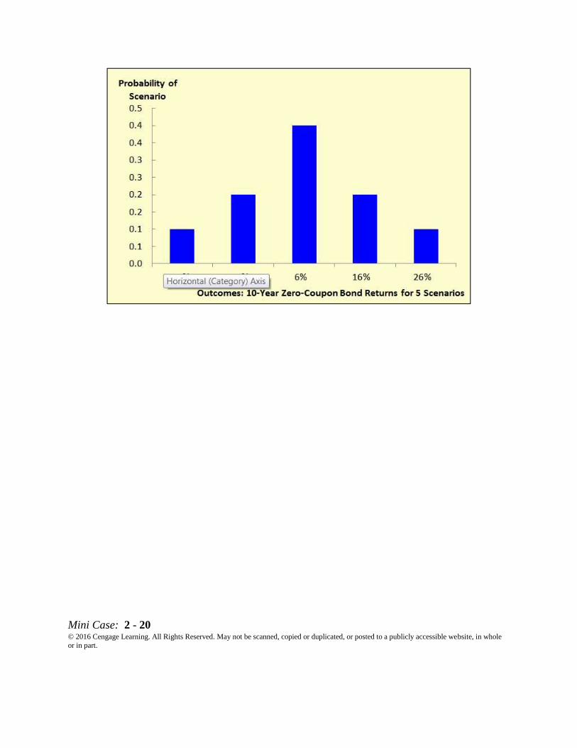
Worst Case 0.10 −14%

Poor Case 0.20 −4%

Most Likely 0.40 6%

Good Case 0.20 16%

Best Case 0.10 26%

1.00

You have also gathered historical returns for the past 10 years for Blandy, Gourmange

Corporation (a producer of gourmet specialty foods), and the stock market.

Historical Stock Returns

Year Market Blandy Gourmange

1 30% 26% 47%

2 7 15 −54

3 18 −14 15

Mini Case: 2 - 19 © 2016 Cengage Learning. All Rights Reserved. May not be scanned, copied or duplicated, or posted to a publicly accessible website, in whole or in part.

4 −22 −15 7

5 −14 2 −28

6 10 −18 40

7 26 42 17

8 −10 30 −23

9 −3 −32 −4

10 38 28 75

Average return: 8.0% ? 9.2%

Standard deviation: 20.1% ? 38.6%

Correlation with the market: 1.00 ? 0.678

Beta: 1.00 ? 1.30

The risk-free rate is 4% and the market risk premium is 5%.

a. What are investment returns? What is the return on an investment that costs

$1,000 and is sold after 1 year for $1,060?

Answer: Investment return measures the financial results of an investment. They may be

expressed in either dollar terms or percentage terms.

The dollar return is $1,60 - $1,000 = $60. The percentage return is $60/$1,000 =

0.06 = 6%.

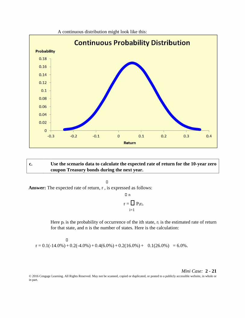
b. Graph the probability distribution for the bond returns based on the 5 scenarios.

What might the graph of the probability distribution look like if there were an

infinite number of scenarios (i.e., if it were a continuous distribution and not a

discrete distribution)?

Answer: Here is the probability distribution for the five possible outcomes:


or in part.


A continuous distribution might look like this:

c. Use the scenario data to calculate the expected rate of return for the 10-year zero

coupon Treasury bonds during the next year.

Answer: The expected rate of return, r , is expressed as follows:

n

r = Piri.

i=1

Here pi is the probability of occurrence of the ith state, ri is the estimated rate of return

for that state, and n is the number of states. Here is the calculation:

r = 0.1(-14.0%) + 0.2(-4.0%) + 0.4(6.0%) + 0.2(16.0%) + 0.1(26.0%) = 6.0%.


or in part.

d. What is stand-alone risk? Use the scenario data to calculate the standard deviation

of the bond’s return for the next year.

Answer: Stand-alone risk is the risk of an asset if it is held by itself and not as a part of a portfolio.

Standard deviation measures the dispersion of possible outcomes, and for a single asset,

the stand-alone risk is measured by standard deviation.

The variance and standard deviation are calculated as follows:

n

σ2 = pi(ri - rˆi)

2

i = 1

2

σ2 = [(0.1) (-0.14 – 0.06)2 + (0.2) (-0.04 – 0.06)2

+ (0.4) (0.06 – 0.06)2

+ (0.2) (0.16 – 0.06)2 + (0.1) (0.26 – 0.06)2]

σ2 = 0.0120

σ = 2 0.0120 = 0.1095 = 10.95%.

e. Your client has decided that the risk of the bond portfolio is acceptable and wishes

to leave it as it is. Now your client has asked you to use historical returns to

estimate the standard deviation of Blandy’s stock returns. (Note: Many analysts

use 4 to 5 years of monthly returns to estimate risk and many use 52 weeks of

weekly returns; some even use a year or less of daily returns. For the sake of

simplicity, use Blandy’s 10 annual returns.)

Answer: The formulas are shown below:

T

. ) r ˆ - r ( p = σ i i 2

i

n

1 = i

2


r t 1

t

r¯Avg = T

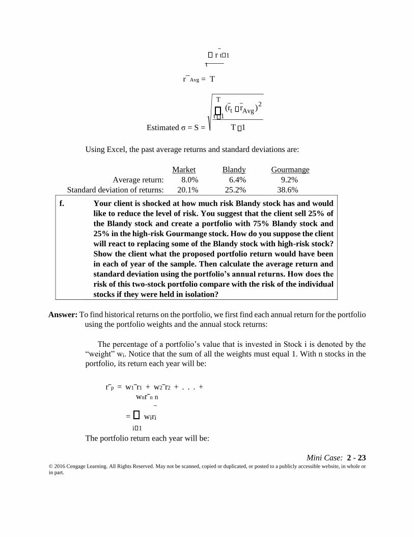
Estimated σ = S =

Using Excel, the past average returns and standard deviations are:

Market Blandy Gourmange

Average return: 8.0% 6.4% 9.2%

Standard deviation of returns: 20.1% 25.2% 38.6%

f. Your client is shocked at how much risk Blandy stock has and would

like to reduce the level of risk. You suggest that the client sell 25% of

the Blandy stock and create a portfolio with 75% Blandy stock and

25% in the high-risk Gourmange stock. How do you suppose the client

will react to replacing some of the Blandy stock with high-risk stock?

Show the client what the proposed portfolio return would have been

in each of year of the sample. Then calculate the average return and

standard deviation using the portfolio’s annual returns. How does the

risk of this two-stock portfolio compare with the risk of the individual

stocks if they were held in isolation?

Answer: To find historical returns on the portfolio, we first find each annual return for the portfolio

using the portfolio weights and the annual stock returns:

The percentage of a portfolio’s value that is invested in Stock i is denoted by the

“weight” wi. Notice that the sum of all the weights must equal 1. With n stocks in the

portfolio, its return each year will be:

r‾p = w1‾r1 + w2‾r2 + . . . +

wnr‾n n

= wiri

i 1

The portfolio return each year will be:

1 T

) r r ( T

1 t

2 Avg t


or in part.

r̅, w r̅,w.r̅.,

r̅, 0.75 r̅, 0.25 r̅.,

Following is a table showing the portfolio’s return in each year. It also shows the

average return and standard deviation during the past 10 years.

Year

Stock Returns

Blandy Gourmange Portfolio

1

26%

47%

31.3%

2 15% -54% -2.3%

3 -14% 15% -6.8%

4 -15% 7% -9.5%

5 2% -28% -5.5%

6 -18% 40% -3.5%

7 42% 17% 35.8%

8 30% -23% 16.8%

9 -32% -4% -25.0%

10 28% 75% 39.8%

Average return: 6.4% 9.2% 7.1%

Standard deviation of returns: 25.2% 38.6% 22.2%

Notice that the portfolio risk is actually less than the standard deviations of the stocks

making up the portfolio.

The average portfolio return during the past 10 years can be calculated as average

return of the 10 yearly returns. But there is another way—the average portfolio return

over a number of periods is also equal to the weighted average of the stock’s average

returns: n

r‾Avg,p = wirAvg,i i 1 This

method is used below: r‾Avg,p = 0.75(6.4%) + 0.25(9.2%) =

7.1%

Note, however, that the only way to calculate the standard deviation of

historical returns for a portfolio is to first calculate the portfolio’s annual historical


returns and then calculate its standard deviation. A portfolio’s historical standard

deviation is not the weighted average of the individual stocks’ standard deviations!

(The only exception occurs when there is zero correlation among the portfolio’s stocks,

which would be extremely rare.)

g. Explain correlation to your client. Calculate the estimated correlation between

Blandy and Gourmange. Does this explain why the portfolio standard deviation

was less than Blandy’s standard deviation?

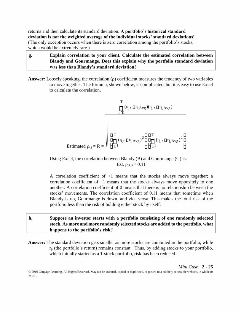
Answer: Loosely speaking, the correlation (ρ) coefficient measures the tendency of two variables

to move together. The formula, shown below, is complicated, but it is easy to use Excel

to calculate the correlation.

Estimated ρi,j = R =

Using Excel, the correlation between Blandy (B) and Gourmange (G) is:

Est. ρB,G = 0.11

A correlation coefficient of +1 means that the stocks always move together; a

correlation coefficient of −1 means that the stocks always move oppositely to one

another. A correlation coefficient of 0 means that there is no relationship between the

stocks’ movements. The correlation coefficient of 0.11 means that sometime when

Blandy is up, Gourmange is down, and vice versa. This makes the total risk of the

portfolio less than the risk of holding either stock by itself.

h. Suppose an investor starts with a portfolio consisting of one randomly selected

stock. As more and more randomly selected stocks are added to the portfolio, what

happens to the portfolio’s risk?

Answer: The standard deviation gets smaller as more stocks are combined in the portfolio, while

rp (the portfolio’s return) remains constant. Thus, by adding stocks to your portfolio,

which initially started as a 1-stock portfolio, risk has been reduced.

T

1 t

2 Avg j, t j,

T

1 t

2 Avg i, t i,

T

1 t Avg j, t j, Avg i, t i,

) r r ( ) r r (

) r r )( r r (


or in part.

In the real world, stocks are positively correlated with one another--if the economy

does well, so do stocks in general, and vice versa. Correlation coefficients between

stocks generally range from +0.5 to +0.7. The average correlation between stocks is

about 0.35. A single stock selected at random would on average have a standard

deviation of about 35 percent. As additional stocks are added to the portfolio, the

portfolio’s standard deviation decreases because the added stocks are not perfectly

positively correlated. However, as more and more stocks are added, each new stock has

less of a risk-reducing impact, and eventually adding additional stocks has virtually no

effect on the portfolio’s risk as measured by σ. In fact, σ stabilizes at about 20 percent

when 40 or more randomly selected stocks are added. Thus, by combining stocks into

well-diversified portfolios, investors can eliminate almost one-half the riskiness of

holding individual stocks. (Note: it is not completely costless to diversify, so even the

largest institutional investors hold less than all stocks. Even index funds generally hold

a smaller portfolio which is highly correlated with an index such as the S&P 500 rather

than hold all the stocks in the index.)

The implication is clear: investors should hold well-diversified portfolios of stocks

rather than individual stocks. (In fact, individuals can hold diversified portfolios

through mutual fund investments.) By doing so, they can eliminate about half of the

riskiness inherent in individual stocks.


i. 1. Should portfolio effects influence how investors think about the risk of individual

stocks?

Answer: Portfolio diversification does affect investors’ views of risk. A stock’s stand-alone risk

as measured by its σ or CV, may be important to an undiversified investor, but it is not

relevant to a well-diversified investor. A rational, risk-averse investor is more

interested in the impact that the stock has on the riskiness of his or her portfolio than

on the stock’s stand-alone risk. Stand-alone risk is composed of diversifiable risk,

which can be eliminated by holding the stock in a well-diversified portfolio, and the

risk that remains is called market risk because it is present even when the entire market

portfolio is held.

i. 2. If you decided to hold a one-stock portfolio and consequently were exposed to more

risk than diversified investors, could you expect to be compensated for all of your

risk; that is, could you earn a risk premium on that part of your risk that you

could have eliminated by diversifying?

Answer: If you hold a one-stock portfolio, you will be exposed to a high degree of risk, but you

won’t be compensated for it. If the return were high enough to compensate you for

your high risk, it would be a bargain for more rational, diversified investors. They

would start buying it, and these buy orders would drive the price up and the return

down. Thus, you simply could not find stocks in the market with returns high enough

to compensate you for the stock’s diversifiable risk.

j. According to the Capital Asset Pricing Model, what measures the amount of risk

that an individual stock contributes to a well-diversified portfolio? Define this

measurement.

Answer: Market risk, which is relevant for stocks held in well-diversified portfolios, is defined as

the contribution of a security to the overall risk of the portfolio. It is measured by a

stock’s beta coefficient. The beta of Stock i, denoted by bi, is calculated as:

bi = i iM


or in part.

M

A stock’s beta can also be estimated by running a regression with the stock’s returns

on the y axis and the market portfolio’s returns on the x axis. The slope of the regression

line gives the same result as the formula shown above.

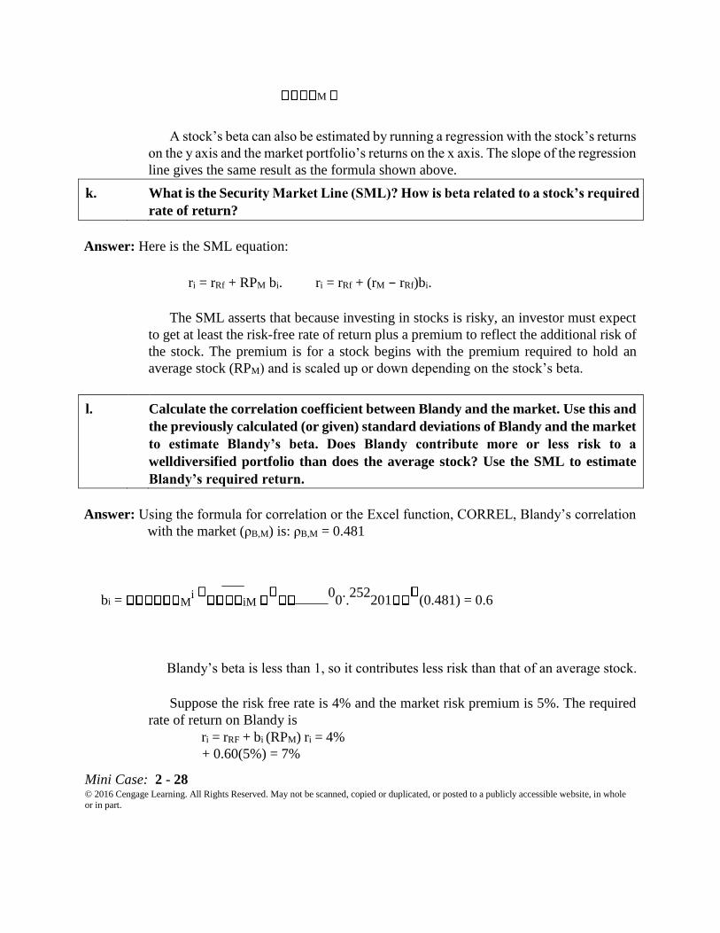
k. What is the Security Market Line (SML)? How is beta related to a stock’s required

rate of return?

Answer: Here is the SML equation:

ri = rRf + RPM bi. ri = rRf + (rM − rRf)bi.

The SML asserts that because investing in stocks is risky, an investor must expect

to get at least the risk-free rate of return plus a premium to reflect the additional risk of

the stock. The premium is for a stock begins with the premium required to hold an

average stock (RPM) and is scaled up or down depending on the stock’s beta.

l. Calculate the correlation coefficient between Blandy and the market. Use this and

the previously calculated (or given) standard deviations of Blandy and the market

to estimate Blandy’s beta. Does Blandy contribute more or less risk to a

welldiversified portfolio than does the average stock? Use the SML to estimate

Blandy’s required return.

Answer: Using the formula for correlation or the Excel function, CORREL, Blandy’s correlation

with the market (ρB,M) is: ρB,M = 0.481

bi = Mi

iM 00..252

201 (0.481) = 0.6

Blandy’s beta is less than 1, so it contributes less risk than that of an average stock.

Suppose the risk free rate is 4% and the market risk premium is 5%. The required

rate of return on Blandy is

ri = rRF + bi (RPM) ri = 4%

+ 0.60(5%) = 7%


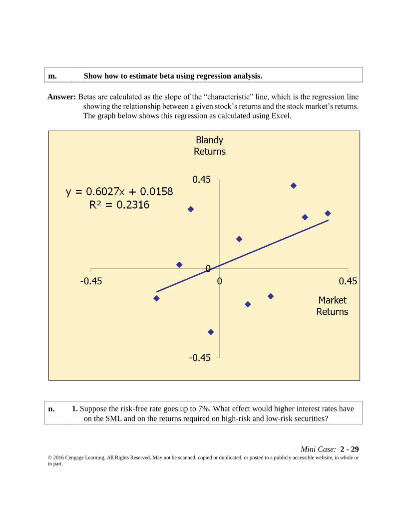
m. Show how to estimate beta using regression analysis.

Answer: Betas are calculated as the slope of the “characteristic” line, which is the regression line

showing the relationship between a given stock’s returns and the stock market’s returns.

The graph below shows this regression as calculated using Excel.

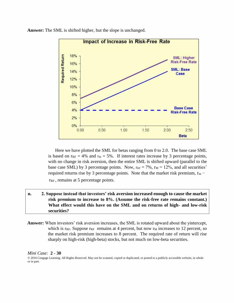
n. 1. Suppose the risk-free rate goes up to 7%. What effect would higher interest rates have

on the SML and on the returns required on high-risk and low-risk securities?


or in part.

Answer: The SML is shifted higher, but the slope is unchanged.

Here we have plotted the SML for betas ranging from 0 to 2.0. The base case SML

is based on rRF = 4% and rM = 5%. If interest rates increase by 3 percentage points,

with no change in risk aversion, then the entire SML is shifted upward (parallel to the

base case SML) by 3 percentage points. Now, rRF = 7%, rM = 12%, and all securities’

required returns rise by 3 percentage points. Note that the market risk premium, rm −

rRF , remains at 5 percentage points.

n. 2. Suppose instead that investors’ risk aversion increased enough to cause the market

risk premium to increase to 8%. (Assume the risk-free rate remains constant.)

What effect would this have on the SML and on returns of high- and low-risk

securities?

Answer: When investors’ risk aversion increases, the SML is rotated upward about the yintercept,

which is rRF. Suppose rRF remains at 4 percent, but now rM increases to 12 percent, so

the market risk premium increases to 8 percent. The required rate of return will rise

sharply on high-risk (high-beta) stocks, but not much on low-beta securities.


o. Your client decides to invest $1.4 million in Blandy stock and $0.6 million in

Gourmange stock. What are the weights for this portfolio? What is the portfolio’s

beta? What is the required return for this portfolio?

Answer: The portfolio’s beta is the weighted average of the stocks’ betas:

bp = 0.7(bBlandy) + 0.3(bGour.)

= 0.7(0.60) + 0.3(1.30)

= 0.81.

There are two ways to calculate the portfolio’s expected return. First, we can use the

portfolio’s beta and the SML:

rp = rRF + bp (RPM)

= 4.0% + 0.81%(5%) = 8.05%.

Second, we can find the weighted average of the stocks’ expected returns: n

rp = wiri

i 1


or in part.

= 0.7(7.0%) + 0.3(10.5%)

= 8.05%.

p. Jordan Jones (JJ) and Casey Carter (CC) are portfolio managers at your firm.

Each manages a well-diversified portfolio. Your boss has asked for your opinion

regarding their performance in the past year. JJ’s portfolio has a beta of 0.6 and

had a return of 8.5%; CC’s portfolio has a beta of 1.4 and had a return of 9.5%.

Which manager had better performance? Why?

Answer: To evaluate the managers, calculate the required returns on their portfolios using the

SML and compare the actual returns to the required returns, as follows:

Portfolio beta =

Portfolio Manager

JJ

CC

0.7

1.4

Risk‐free rate = 4%

4%

Market risk premium

= 5%

5%

Portfolio required

return = 7.50%

11.00%

Portfolio actual return =

8.50%

9.50%

Over (Under) Performance =

1.00%

‐1.50%

Notice that JJ’s portfolio had a higher return than investors required (given the risk

of the portfolio) and CC’s portfolio had a lower return than expected by investors.

Therefore, JJ had the better performance.

q. What does market equilibrium mean? If equilibrium does not exist, how will it be

established?


Answer: Market equilibrium means that marginal investors (the ones whose trades determine

prices) believe that all securities are fairly priced. This means that the market price of

a security must equal the security’s intrinsic value (intrinsic value reflects the size,

timing, and risk of the future cash flows):

Market price = Intrinsic value

Market equilibrium also means that the expected return a security must equal its

required return (which reflects the security’s risk).

= r

If the market is not in equilibrium, then some assets will be undervalued and/or

some will be overvalued. If this is the case, traders will attempt to make a profit by

purchasing undervalued securities and short-selling overvalued securities. The

additional demand for undervalued securities will drive up their prices and the lack of

demand for overvalued securities will drive down their prices. This will continue until

market prices equal intrinsic values, at which point the traders will not be able to earn

profits greater than justified by the assets’ risks.

r. What is the Efficient Markets Hypothesis (EMH) and what are its three forms?

What evidence supports the EMH? What evidence casts doubt on the EMH?

Answer: The EMH is the hypothesis that securities are normally in equilibrium, and are “priced

fairly,” making it impossible to “beat the market.”

Weak-form efficiency says that investors cannot profit from looking at past

movements in stock prices--the fact that stocks went down for the last few days is no

reason to think that they will go up (or down) in the future. This form has been proven

by empirical tests, even though people still employ “technical analysis.”

Semistrong-form efficiency says that all publicly available information is reflected in

stock prices, hence that it won’t do much good to pore over annual reports trying to

find undervalued stocks. This one is (I think) largely true, but superior analysts can still

obtain and process new information fast enough to gain a small advantage.

Strong-form efficiency says that all information, even inside information, is embedded

in stock prices. This form does not hold--insiders know more, and could take advantage

of that information to make abnormal profits in the markets. Trading on the basis of

insider information is illegal.

Most empirical evidence supports weak-form EMH because very few trading

strategies consistently earn in excess of the CAPM prediction, with two possible

exceptions that earn very small excess returns: (1) short-term momentum and (2)

longterm reversals.


or in part.

Most empirical evidence supports the semistrong-form EMH. For example, the vast

majority of portfolio managers do not consistently have returns in excess of CAPM

predictions. There are two possible exceptions that earn excess returns: (1) small

companies and (2) companies with high book-to-market ratios.

In addition, there are times when a market becomes overvalued. This is often called

a bubble. Bubbles are hard to burst because trading strategies expose traders to possible

big negative cash flows if the bubble is slow to burst.

© 2016 Cengage Learning. All Rights Reserved. May not be scanned, copied or duplicated, or posted to a publicly accessible website, in whole

or in part.

Web Appendix 2B Calculating Beta Coefficients With a Financial Calculator

Solutions to Problems

2B-1 a. rY(%)

rM (%)

b = Slope = 0.62. However, b will depend on students’ freehand line. Using a

calculator, we find b = 0.6171 ≈ 0.62.

b. Because b = 0.62, Stock Y is about 62% as volatile as the market; thus, its relative risk

is about 62% that of an average stock.

c. 1. Stand-alone risk as measured by would be greater, but beta and hence systematic

(relevant) risk would remain unchanged. However, in a 1-stock portfolio, Stock Y

would be riskier under the new conditions.

2. CAPM assumes that company-specific risk will be eliminated in a portfolio, so the risk

premium under the CAPM would not be affected. However, if the scatter were

wide, we would not have as much confidence in the beta, and this could increase

the stock's risk and thus its risk premium.

d. 1. The stock's variance and would not change, but the risk of the stock to an investor

holding a diversified portfolio would be greatly reduced, because it would now have a

negative correlation with rM.

40

30

20

10

-30 -20 -10 10 20 30 40


or in part.

Web Solutions: 2B - 36

2. Because of a relative scarcity of such stocks and the beneficial net effect on portfolios

that include it, its “risk premium” is likely to be very low or even negative.

Theoretically, it should be negative.

e. The following figure shows a possible set of probability distributions. We can be

reasonably sure that the 100-stock portfolio comprised of b = 0.62 stocks as described

in Condition 2 will be less risky than the “market.” Hence, the distribution for

Condition 2 will be more peaked than that of Condition 3.

We can also say on the basis of the available information that Y is smaller than

M; Stock Y’s market risk is only 62% of the “market,” but it does have company-

specific risk, while the market portfolio does not, because it has been diversified away.

However, we know from the given data that Y = 13.8%, while M = 19.6%. Thus, we

have drawn the distribution for the single stock portfolio more peaked than that of the

market. The relative rates of return are not reasonable. The return for any stock should

be ri = rRF + (rM – rRF)bi.

Stock Y has b = 0.62, while the average stock (M) has b = 1.0; therefore,

ry = rRF + (rM – rRF)0.62 < rM = rRF + (rM – rRF)1.0.

A disequilibrium exists—Stock Y should be bid up to drive its yield down. More likely,

however, the data simply reflect the fact that past returns are not an exact basis for

9.8

K r 100

K r M

K r Y


or in part.


expectations of future returns.

f. The expected return could not be predicted with the historical characteristic line

because the increased risk should change the beta used in the characteristic line.

g. The beta would decline to 0.53. A decline indicates that the stock has become less

risky; however, with the change in the debt ratio the stock has actually become more

risky. In periods of transition, when the risk of the firm is changing, the beta can yield

conclusions that are exactly opposite to the actual facts. Once the company's risk

stabilizes, the calculated beta should rise and should again approximate the true beta.

2B-2 a.

The slope of the characteristic line is the stock’s beta coefficient.

Rise ri

Slope = .

Run rM

SlopeA = BetaA = = 1.0.

SlopeB = BetaB = = 0.5.

-5

5

10

15

20

25

30

35

5 10 15 20 25 30 35

r i ( % )

r M ) ( %

Stock A

Stock B


or in part.

b. ˆrM = 0.1(-14%) + 0.2(0%) + 0.4(15%) + 0.2(25%) + 0.1(44%) = -

1.4% + 0% + 6% + 5% + 4.4% = 14%.


The graph of the SML is as follows:

The equation of the SML is thus: ri = rRF + (rM – rRF)bi = 9% + (14%

– 9%)bi = 9% + (5%)bi.

c. Required rate of return on Stock A:

rA = rRF + (rM – rRF)bA = 9% + (14% – 9%)1.0 = 14%.

Required rate of return on Stock B:

rB = 9% + (14% – 9%)0.5 = 11.50%.

d. Expected return on Stock C = ˆrC = 18%.

Return on Stock C if it is in equilibrium:

rC = rRF + (rM – rRF)bC = 9% + (14% – 9%)2 = 19% 18% = ˆrC.

A stock is in equilibrium when its required return is equal to its expected return.

Stock C’s required return is greater than its expected return; therefore, Stock C is not

SML r i

r RF = 9%

E(r M ) = 14%

b 1.0


or in part.

in equilibrium. Equilibrium will be restored when the expected return on Stock C is

driven up to 19%. With an expected return of 18% on Stock C, investors should sell it,

driving its price down and its yield up.


chapter 2 risk and return: part i€¦ · in theory, investors should be concerned only with...

Documents