2017-03-233:42pm 1

Chapter2.Newworldsversusscaling:fromvanLeeuwenhoektoMandelbrot

2.1ScaleboundthinkingandthemissingquadrillionWe just tookavoyage throughscales,noticing structures in cloudphotographsand

wiggles on graphs. Collectively these spanned ranges of scale over factors of billions inspaceandbillionsofbillions in time. Weare immediately confrontedwith thequestion:howcanweconceptualizeandmodelsuchfantasticvariation?

Twoextremeapproacheshavedeveloped,forthemomentIwillcallthedominantonethe “new worlds” view after Antoni van Leeuwenhoek (1632-1723), who developed apowerfulearlymicroscope,theother,theself-similar(scaling)viewbyBenoitMandelbrot(1924-2010)thatIdiscussinthenextsection.Myownview-scalingbutwiththenotionofscaleitselfanemergentproperty-isdiscussedinch.3.

WhenvanLeeuwenhoekpeeredthroughhismicroscopea,inhisamazementheissaidto have discovered a “new world in a drop of water”: “animalcules”, the first micro-organismsb(fig.2.1).Sincethen,theideathatzoominginwillrevealsomethingtotallynewhas become second nature: in the 21st century atom-imagingmicroscopes are developedprecisely because of the promise of such newworlds. The scale-by-scale “newness” ideawas graphically illustrated by K. Boeke’s highly influential book “Cosmic View” (1957)which starts with a photograph of a girl holding a cat, first zooming away showing thesurroundingvastreachesofouterspace,andthenzoominginuntilreachingthenucleusofan atom. The book was incredibly successful, and was included in Mortimer Adler's“Gateway to the Great Books” (1963), a 10 volume series featuring works by Aristotle,Shakespeare,Einsteinandothers.In1968,twofilmswerebasedonBoeke’sbook:“CosmicZoom”cand“PowersofTen”(1968d,re-releasedin1977e)whichencouragedtheideathatnearly every power of ten in scale hosted different phenomena. More recently (2012),there’seventheinteractiveCosmicEye,appfortheiPad,iPhone,oriPod.Ina1981paper,Mandelbrot coined the term “scalebound” for this “New Worlds” view, a convenientshorthandfthatIusefrequentlybelowg.

While“PowersofTen”wasproselytizingthenewworldsviewtoanentiregeneration,therewereotherdevelopmentsthatpushedscientificthinkinginthesamedirection.Inthe1960’s,longiceandoceancoreswererevolutionizingclimatesciencebysupplyingthefirstquantitativedataatcentennial,millennialandlongertimescales. Thiscoincidedwiththe

aTheinventorofthefirstmicroscopeisnotknown,butvanLeuwenhoek’swasmorepowerful,uptoabout300timesmagnification.bRecenthistoricalresearch indicatesthatRobertHookemayin facthaveprecededvanLeeuwenhoek,butthelatterisusuallycreditedwiththediscovery.cProducedbytheNationalFilmBoardofCanada.dByCharlesandRayEames.eThere-releasehadthesubtitle:“AFilmDealingwiththeRelativeSizeofThingsintheUniverseandtheEffectofAddingAnotherZero”andwasnarratedbyP.Morrison.Morerecently,thesimilar“CosmicVoyage”(1996),appearedinIMAXformat.fHewroteitashere,asoneword,asasingleconcept.gHewaswritinginLeonardo,toanaudienceofarchitects:“Iproposethetermscaleboundtodenoteanyobject,whether innatureoronemadebyanengineeroranartist, forwhichcharacteristicelementsofscale,suchaslengthandwidth,arefewinnumberandeachwithaclearlydistinctsize”:1 Mandelbrot,B.Scaleboundorscalingshapes:ausefuldistinctioninthevisualartsandinthenaturalsciences.Leonardo14,43-47(1981).

2017-03-233:42pm 2

development of practical techniques to decompose a signal into oscillating components:“spectral analysis”. While ithadbeenknownsince JosephFourier (1768-1830) thatanytime series may be written as a sum of sinusoids, applying this idea to real data wascomputationally challenging and in atmospheric science had been largely confined to thestudyof turbulence. Thebreakthroughwasthedevelopmentof fastcomputerscombinedwiththediscoveryofthe“FastFourierTransform”(FFT)algorithmh(1968).

ThebeautyofFourierdecompositionisthateachsinusoidhasanexact,unambiguoustimescale: itsperiod(theinverseof its frequency)isthelengthoftimeittakestomakeafull oscillation (fig. 2.2a, upper left for examples). Fourier analysis thus provides asystematicwayofquantifyingthecontributionofeachtimescaletoatimeseries.Fig.2.2aillustrates this for the Weierstrass function which in this example, is constructed bysummingsinusoidswithfrequenciesincreasingbyfactorsoftwosothatthenthfrequencyisω =2n. Fig2.2a (upper left) shows the result forH =1/3with all the termsupuntil 128cyclespersecond(upperrow); theamplitudesdecreaseby factorsof2-H (here=0.79)sothatthenthamplitudeis2-nH. Eliminatingn,wefindthepowerlawrelationA=ω-H. Moregenerallyforascalingprocess,wehave:

Spectrum=(frequency)-β

Whereβistheusualnotationforthe“spectralexponent”i.Thespectrumisthesquareoftheamplitude, so that in this (discrete) examplejwe have β =2H. The spectrum of theWeierstrassfunctionisshowninfig.2.2abottomrow(left)asadiscreteseriesofdots,onefor each of the 8 sinusoids in the upper left construction. On the bottom row (right)weshowthesamespectrumbutonalogarithmicplotonwhichpowerlawsarestraightlines.Ofcourse,intherealworld-unlikethisacademicexample-thereisnothingspecialaboutpowersof2sothatallfrequencies–acontinuum-arepresent.

TheWeierstrassfunctionwascreatedbyaddingsinusoids:Fouriercomposition.Nowtakeamessypieceofdata–forexamplethemultifractalsimulationofthedataseries(lowerleftinfig.1.3):ithassmall,mediumandlargewiggles.Toanalyzeitweneedtheinverseofcomposition,andthisiswheretheFFTishandy.Inthiscase,byconstruction,weknowthatall the wiggles are generated randomly by the process; that they are unimportant.However, ifwe hadno knowledge – or only a speculation - about of themechanism thatproduced it,wewouldwonder: do thewiggles hide signatures of important processes ofinterest,oraretheysimplyuninterestingdetailsthatshouldbeaveragingoutandignored?

hThe speed-up due to the invention of the FFT is huge: even for the relatively short series in fig. 1.3 (2048points)itisaboutafactorofonehundred.InGCM’sitacceleratescalculationsbyfactorsofmillions.iThenegativesignisusedtosothatintypicalsituations,βispositive.jInthemoreusualcaseofcontinuousspectra,wehaveβ =1+2Hpossiblywithcorrectionswhenintermittencyisimportant.

2017-03-233:42pm 3

Fig.2.1:AntonivanLeuwenhoekdiscovering“animalcules”(micro-organisms),circa1675.Fig.2.2bshowsthespectrumofthemultifractalsimulation(fig.1.3lowerleft)forall

periodslongerthan10milliseconds.Howdoweinterprettheplot?Oneseesthreestrongspikes,atfrequenciesof12,28and41cyclespersecond(correspondingtoperiodsof1/12,1/28 and 1/41 of a second, about 83, 35, 24 milliseconds). Are they signals of someimportantfundamentalprocessoraretheyjustnoise?

Naturally,thisquestioncanonlybeansweredifwehaveamentalmodelofhowtheprocessmightbegenerated,andthisiswhereitgetsinteresting. Firstofall,considerthecasewherewehaveonlyasingleseries.Ifweknewthesignalwasturbulent(asitwasforthetopdataseries),thenturbulencetheorytellsusthatwewouldexpectallthefrequenciesin awide continuumof scales tobe important, and furthermore, that at leastonaverage,that their amplitudes should decay in a power law manner (as with the Weierstrassfunction). But the theory only tells us the spectrum that wewould expect to find if weaveragedovera largenumberof identical experimentsk(eachonewithdifferent “bumps”andwiggles,butfromthesameoverallconditions).Infig.2.2b,thisaverageisthesmoothbluecurve.

Butinthefigure,weseethatthereareapparentlylargedeparturesfromthisaverage.Arethesedeparturesreallyexceptionalorarethesejust“normal”variationsexpectedfromrandomlychosenpiecesofturbulence?Beforethedevelopmentofcascademodelsandthediscovery ofmultifractals in the1970’s and80’s, turbulence theorywouldhave ledus toexpect that theupanddownvariationsaboutasmooth line throughthespectrumshouldroughlyfollowthe“bellcurve”. Ifthiswasthecase,thenthespectrumshouldnotexceedthe bottom red curvemore than 1%of the time and the top curvemore than one in tenbilliontimes. Yet,weseethateventhis1/10,000,000,000curveisexceededtwiceinthissinglebutnonexceptional simulationl. Hadweencountered this series inanexperiment,

kAn“ensemble”or“statistical”average.lIadmitthattomakemypoint,Imade500simulationsofthemultifractalprocessinfig.1.3andthensearchedthroughthefirst50tofindtheonewiththemoststrikingvariation.Butthiswasbynomeansthemostextremeofthe500andifthestatisticshadbeenfromthebellcurve,thentheextremepointinthespectruminfig.2.3wouldhavecorrespondedtoaprobabilityofonein10trillion,sothatmyslightcheatingintheselectionprocesswouldstillhavebeenextremelyunlikelytohavecausedtheresult!

2017-03-233:42pm 4

turbulencetheory itselfwouldprobablyhavebeenquestioned–as it indeed itrepeatedlywas(andstillis).Failuretofullyappreciatethehugevariabilitythatisexpectedinturbulentprocesses and continued embrace of inappropriate bell curve type paradigms hasspuriouslysheddiscreditonmanyattemptsatestablishingturbulent lawsandhasbeenamajorobstacleintheirunderstanding.

Fig. 2.2a: Upper left: The first eight contributions to the Weierstrass function (displaced in thevertical for clarity). Sinusoidswith frequenciesof1, 2, 4, 8, 16, 32,64,128 cyclesper second (thetimetisinseconds).Upperright:Sinusoidswithfrequenciesof2,4,8,16,32,64,128,cyclespersecond,stretchedbyafactor1.25intheverticalandafactoroftwointhehorizontal.Thesum(top)isthesameasthatontheleftbutismissingthehighestfrequencydetail(seethediscussionalittlelater).Lower left: The spectrumon a linear-linear scale each point indicating the contribution (squared)andthefrequency.Lowerright:Thesameaslowerleftbutonalogarithmicplot(itisnowlinear).

In conclusion, until the 1980’s even if we knew that the series came from anapparentlyroutineturbulentwindtraceontheroofofthephysicsbuilding,wewouldstillhaveconcludedthatthebumpswereindeedsignificant.

Butwhatwouldbeourinterpretationifinsteadfig.2.2bwasthespectrumofaclimateseries?Wewouldhavenogoodtheoryofthevariabilityandwewouldtypicallyonlyhaveasingletrace.

Let’staketheexampleofanicecorerecord.Theseriesitselfwaslikelytheproductofa near heroic scientific effort, possibly involving months in freezing conditions near thesouthpole. Thesamplewouldfirstbecoredandthentransportedtothelab. Thiswouldhave been followed by a painstaking sampling and analysis of the isotopic composition

��� ��� ��� ��� ������������(�)

��� ��� ��� ��� �������������(�)

�� �� �� �� ��� ��� ω����������������(ω)

��� ��� ��� ��� ���ω

-���-���-���-���-���-���-���

����(ω)

2017-03-233:42pm 5

usingamassspectrometer,thenadigitizationoftheresult.Carefulcomparisonwithothercoresorwith ice flowmodelswouldeventuallyestablisha chronology. At thispoint, theresearcherwouldbeeagerforaquantitativelookatwhatshehadfound.Iftheblackcurvein fig. 2.2b was the spectrum of such a core, how would she react to the bumps in thespectrum? Unlike the turbulence situationwhere therewas some theory, an early corewouldhavehad littlewithwhich to compare it. This is thepointwhere thenewworldsview could easily influence the researcher’s resultsm. She would be greatly tempted toconclude that the spikes were so strong, so far from the bell curve theory that theyrepresented real physical oscillations occurring over a narrow range of time scales. Shewould also remark that the twomain bumps in the spectrum involve several successivefrequencies,andaccordingtousualstatisticalassumptions,“backgroundnoise”shouldnotbecorrelatedinthisway. Thiswidebumpwouldstrengthentheinterpretationthattherewasahiddenoscillatoryprocessatworkn.Armedwiththeseriesofbumps,shemightstarttospeculateaboutpossiblephysicalmechanismstoexplainthem.

Fig.2.2b:Black:theFourierspectrumofthechangesinwindspeedinthe1secondlongsimulationshownat thebottom left of fig. 1.3, showing theamplitudesoof the first100 frequencies (ω). Theupperleftisthusforonecycleoverthelengthofthesimulation,i.e.onecyclepersecond,aperiodofonesecond.Thefarrightshowsthevariabilityat100cyclespersecondgivingtheamplitudeofthewigglesat10milliseconds (higher frequencieswerenot shown for clarity). Thebrownshows theaverageover500randomserieseachidenticaltothatinfig.1.3:asexpected,itisnearlyexactlythetheoretical(scaling)powerlaw(blue,thetwovirtuallyontopofeachother).Thethreeredcurvesshowthetheoretical1%,oneinamillionandoneintenbillionextremefluctuationlimits(bottomtotop)determinedbyassumingthatthespectrumhasbellcurve(Gaussian)probabilities.

Weshouldthusnotbesurprisedtolearnthatthe1970’switnessedarashofpapers

basedonspectraresemblingthatoffig.2.2b:oscillatorsweresuddenlyubiquitousp.Itwas

mAlternatively, theremightbe incorrect theories that couldbe spuriously supportedbyunfortunatelyplacedrandomspectralbumps,andmuchtimewouldbewastingchasingblindalleys.nAccording to standard assumptions that –if only demonstrated by this example are clearly inappropriate -successivefrequenciesshouldbestatisticallyindependentofeachother.oThespectrumisactuallytheensembleaverageofthesquaresoftheabsoluteamplitudes.Itwaswindowed”inordertoavoidspurious“spectralleakage”thatcouldartificiallysmearoutthespectrum.pI could alsomention the contribution of “Box-Jenkins” techniques (1970) to bolstering scaleboundblinkers.Thesewereoriginallyengineeringtools foranalyzingandmodelingstochasticprocessesbasedontheapriori

�� �� �� �� ���ω�

���

���

���

���

����(ω)

2017-03-233:42pm 6

inthiscontextthatMurrayMitchell5(1928-1990)famouslymadethefirstexplicitattempttoconceptualizetemporalatmosphericvariability(fig2.3a).Mitchell’sambitiouscompositespectrum ranged from hours to the age of the earth (≈4.5x109 to 10-4 years, bottom, fig.2.3a). In spite of his candid admission that this was mostly an “educated guess”, andnotwithstanding the subsequent revolution in climate and paleoclimate data, over fortyyears later it has achieved an iconic status and is still regularly cited and reproduced inclimatepapersandtextbooks6,7,8. Itscontinuing influence isdemonstratedby theslightlyupdatedversionshowninfig.2.3bthat(until2015)adornedNOAA’sNationalClimateDataCenter (NCDC) paleoclimate web siteq. The site was surprisingly forthright about thefigure’sideologicalcharacter.Whileadmittingthat“insomerespectsitovergeneralizesandover-simplifiesclimateprocesses”,itcontinues:“…thefigureisintendedasamentalmodeltoprovideageneral"powersoften"overviewofclimatevariability,andtoconveythebasiccomplexitiesofclimatedynamicsforageneralsciencesavvyaudience.”Noticetheexplicitreferencetothe“powersoften”mindsetoverfiftyyearsafterBoeke’sbookr.

Certainly the continuing influence of Mitchell’s figure has nothing to do with itsaccuracy.Withinfifteenyearsofitspublication,twoscalingcomposites(closetoseveralofthose shown in fig. 2.3 a), over the ranges 1 hr to 105 yrs, (see fig. 2.10 for the relatedfluctuations) and 103 to 108 yrs, already showed astronomical discrepancies9, 10. In thefigure, we have superposed the spectra of several of the series analysed in ch. 1; thedifferencewithMitchell’soriginalisliterallyastronomical.Whereasovertherange1hrto109yrs,Mitchell’sbackgroundvariesbyafactor≈150,thespectrafromrealdataimplythatthe true range is a factorof a quadrillions(1015),NOAA’s fig. 2.3b extends this errorby afurtherfactoroftent.

Writing a decade and a half after Mitchell, leading climatologists Shackelton andImbrie10laconicallynotedthattheirownspectrumwas“muchsteeperthanthatvisualisedbyMitchell”,aconclusionsubsequentlyreinforcedbyseveralscalingcomposites11,12.Overat leastasignificantpartof thisrange,Wunsch13 furtherunderlined itsmisleadingnatureby demonstrating that the contribution to the variability from specific frequenciesassociatedwithspecific“spikes”(presumedtooriginateinoscillatoryprocesses)wasmuchsmallerthanthecontributionduetothecontinuum.

JustasvanLeuwenhookpeeredthroughthefirstmicroscopeanddiscoveredanewworld,today,weautomaticallyanticipatefindingnewworldsbyzoominginoroutofscale.Itisascientificideologysopowerfulthatevenquadrillionsdonotshakeit.

scaleboundassumptionthatthecorrelationsdecayedinanexponentialmanner.Thisespeciallycontributedtoscaleboundthinkinginprecipitationandhydrologyseeforexampletheinfluentialpublications:2 Zawadzki,I.Statisticalpropertiesofprecipitationpatterns.JournalofAppliedMeteorology12,469-472(1973).3 Bras,R. L.&Rodriguez-Iturbe, I.Rainfall generation: anonstationary timevaryingmultidimensionalmodel.WaterResourcesResearch12,450-456(1976);4Bras,R.L.&Rodriguez-Iturbe,I.RandomFunctionsandHydrology.(Addison-WesleyPublishingCompany,1985).qThesiteexplicitlyacknowledgesMitchell’sinfluence.rIf this were not enough, the site adds a further gratuitous interpretation: assuring any sceptics that just“because a particular phenomenon is called an oscillation, it does not necessarilymean there is a particularoscillator causing the pattern. Some prefer to refer to such processes as variability.” Since any time serieswhether produced by turbulence, the stock market or a pendulum can be decomposed into sinusoids: thedecompositionhasnophysicalcontentperse,yetwearetoldthatvariabilityandoscillationsaresynonymous.sIn fig. 2.11a,we plot the same information but in real space and find thatwhereas the RMS fluctuations at5.53x108yearsare≈±10KsothatextrapolatingGaussianwhitenoiseovertherangeimpliesavalue≈10-6K,i.e.itisinerrorbyafactor≈107.tIf we attempt to extend Mitchell’s picture to the dissipation scales (at frequencies a million times higher,correspondingtomillisecondvariability),thespectralrangewouldincreasebyanadditionalfactorofabillion.

2017-03-233:42pm 7

Mitchell’s scalebound view led to a framework for atmospheric dynamics thatemphasized the importanceof numerousprocesses occurring atwell defined time scales,thequasiperiodic“foreground”processesillustratedasbumps–thesignals-onMitchell’snearly flat background that was considered to be an unimportant noiseu. Although inMitchell’soriginalfigure,theletteringisdifficulttodecipher,fig.2.3bspellsthemoutmoreclearlywithnumerousconventionalexamples.Forexample,theQBOisthe“Quasi-BiennalOscillation”, ENSO is the “El Nino Southern Oscillation”, the PDO is the “Pacific DecadalOscillation” and the NAO is the “North Atlantic Oscillation”. At longer time scales, theDansgaards-OescherandMilankovitchandtectonic“cycles”vwillbediscussedinch.4.Thepointhereisnotthattheseprocesses,mechanismsarewrongorinexistent,itisratherthattheyonlyexplainasmallfractionoftheoverallvariability.Even the nonlinear revolution was affected by scalebound thinking. This includedatmosphericapplicationsof lowdimensionaldeterministicchaos. When itwasappliedtoweather and climate, the spectral bumps were associated with specific chaos models,analysedwiththehelpofthedynamicalsystemsmachineryofbifurcations,limitcyclesandthe likew. Of course – asdiscussedbelow - from the alternative scaling, turbulence view,wide range continuum spectra are generic results of systems with large numbers ofinteracting components (“degrees of freedom”) - “stochastic chaos” 15 – and areincompatiblewith theusualsmallnumberof interactingcomponents (“lowdimensional”)deterministicchaos.Incredibly,afamouspaperpublishedinNatureevenclaimedthatfourinteractingcomponents(!)wereenoughtodescribeandmodeltheclimate16.Similarly,thespectrawill be scaling - i.e. power laws –whenever there are no dynamically importantcharacteristicscalesorscalebreaksx(ch.3).

uMitchellactuallyassumedthathisbackgroundwaseitherawhitenoiseorovershortranges,sums(integrals)ofawhitenoise.vThefigurereferstotheseas“cycles”ratherthanoscillations,perhapsbecausetheyarebroader.wMorerecentlyupdatedwiththehelpofstochastics:the“randomdynamicalsystems”approach,seee.g.:14 Chekroun,M.D., Simonnet,E.&Ghil,M. StochasticClimateDynamics:RandomAttractorsandTime-dependentInvariantMeasuresPhysicaD240,1685-1700(2010).8 Dijkstra,H.NonlinearClimateDynamics.(CambridgeUniversityPress,2013).xAlthough in themore recent randomdynamical systems approach, the driving noisemay be viewed as theexpressionofalargenumbersofdegreesoffreedom,thisinterpretationisonlyjustifiedifthereisasignificantscalebreakbetweenthescalesofthenoiseandoftheexplicitlymodelleddynamics,itisnottriviallycompatiblewithscalingspectra.

2017-03-233:42pm 8

Fig.2.3a:AcomparisonofMitchell’srelativescale,“educatedguess”ofthespectrum(grey,bottom5)with modern evidence from spectra of a selection of the series displayed in fig. 1.4 (the plot islogarithmic in both axes). There are three sets of red lines; on the far right, the spectra from the1871-2008 20CR (at daily resolution) quantifies the difference between the globally averagedtemperature(bottom)andlocalaverages(2ox2o,top).

Thespectrawereaveragedoverfrequencyintervals(10perfactorofteninfrequency),thus“smearing out” the daily and annual spectral “spikes”. These spikes have been re-introducedwithout this averaging, and are indicated by green spikes above the red daily resolution curves.Using thedaily resolutiondata, the annual cycle is a factor≈1000 above the continuum,whereasusinghourlyresolutiondata,thedailyspikeisafactor≈3000abovethebackground.Alsoshownistheotherstrikingnarrowspectralspikeat(41kyrs)-1(obliquity;≈afactor10abovethecontinuum),this is shown in dashed green since it is only apparent over the period 0.8 - 2.56MyrBP (beforepresent).

The blue lines have slopes indicating the scaling behaviours. The thin dashed green linesshowthetransitionperiodsthatseparateouttheregimesdiscussedindetailinch.3;theseareat20days,50yrs,80,000yrs,and500,000yrs. Mitchell’soriginal figurehasbeen faithfullyreproducedmanytimes(withthesameadmittedlymediocrequality).Itisnotactuallyveryimportanttobeabletoreadtheletteringnearthespikes,ifneededtheycanseeninfig.2.3bwhichwasinspiredbyit.

10-10

1

10-5

105

Log 1

0E(ω)

K2yr

1015

Macroclim

ate

β =

-0.6

β = 0.6

megaclimate macroweather weather

β = 1.8

β = 1.8

β = 1.8

β = 0.2

climate

E ω( ) ≈ ω−β

10410210-210-510-610-9 Log10ω(yr)-1

2017-03-233:42pm 9

Fig.2.3b:TheupdatedversionofMitchell’s spectrumreproduced fromNOAA’sNCDCpaleoclimateweb sitey. The “background” on this paleo site is perfectly flat; hence in comparison with theempiricalspectruminfig.2a,itisinerrorbyanoverallfactor≈1016.

***

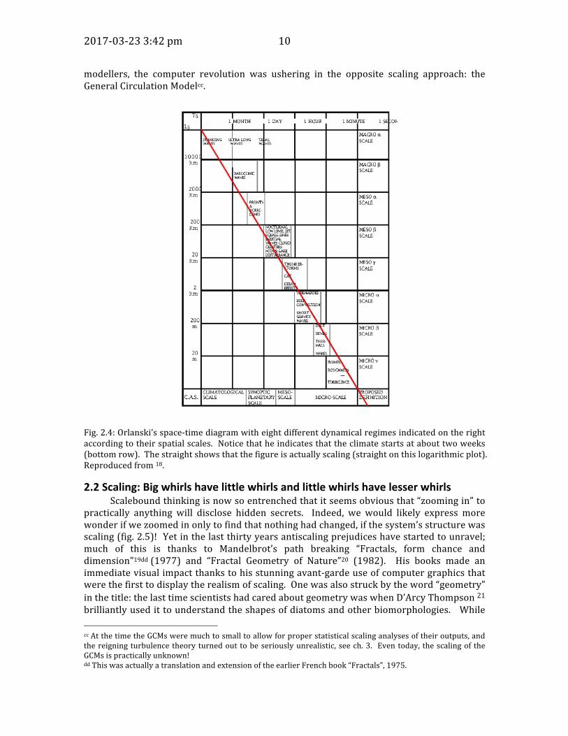
At weather scales, and at virtually the same time as Mitchell’s scaleboundframework for temporal variability, Isidoro Orlanski proposed a scalebound spatialclassification of atmospheric phenomena by powers of ten (fig. 2.4)17. The figure is areproduction of Orlanski’s phenomenological space-time diagramzwith eight differentdynamical regimes indicated on the right according to their spatial scales. The diagramdoesmorethanjustclassifyphenomenaaccordingtotheirsize,italsorelatestheirsizestotheir lifetimesaa. Along the diagonal, various pre-existing conventional phenomena areindicated including fronts, hurricanes, tornadoes and thunderstorms. The straight lineembellishmentwasaddedbycolleaguesandIin199718andshowsthatthefigureisactuallyscalingnotscalebound!Thisisbecausestraightlinesonlogarithmicplotssuchasthisarepowerlaws;moreonthisbelow.

AtthetimeofOrlanski’sclassification,meteorologywasalreadylargelyscalebound.Thiswaspartlyduetoitsneartotaldivorcefromprimarilyscalingturbulencetheorybb,andalso it was due to its heritage from the older more qualitative traditions of “synoptic”meteorologyandoflinearizedapproaches-thesebeingtheonlyonesavailableinthepre-computerera. Orlanski’s classification therefore rapidlybecamepopularasa systematicrationalizationofanalreadystronglyphenomenologicallyscaleboundapproach.ItisironicthatjustasOrlanskitriedtoperfecttheoldscaleboundapproach,andunbeknownsttothe

yThepageishassincebeentakendown.zSometimescalled“Stommeldiagrams”afterHenryStommelwhoproducedsuchdiagramsinoceanography.aaNoticethatheindicatesthattheclimatestartsatabouttwoweeks(bottomrow).bbAll the turbulence theories were scaling, the question was whether one or two ranges were required; wediscussthisindetailinch.3.

2017-03-233:42pm 10

modellers, the computer revolution was ushering in the opposite scaling approach: theGeneralCirculationModelcc.

Fig.2.4:Orlanski’sspace-timediagramwitheightdifferentdynamicalregimesindicatedontherightaccordingtotheirspatialscales.Noticethatheindicatesthattheclimatestartsatabouttwoweeks(bottomrow).Thestraightshowsthatthefigureisactuallyscaling(straightonthislogarithmicplot).Reproducedfrom18.

2.2Scaling:BigwhirlshavelittlewhirlsandlittlewhirlshavelesserwhirlsScaleboundthinkingisnowsoentrenchedthatitseemsobviousthat“zoomingin”to

practically anything will disclose hidden secrets. Indeed, we would likely express morewonderifwezoomedinonlytofindthatnothinghadchanged,ifthesystem’sstructurewasscaling(fig.2.5)!Yetinthelastthirtyyearsantiscalingprejudiceshavestartedtounravel;much of this is thanks to Mandelbrot’s path breaking “Fractals, form chance anddimension”19dd(1977) and “Fractal Geometry of Nature”20 (1982). His books made animmediatevisualimpactthankstohisstunningavant-gardeuseofcomputergraphicsthatwerethefirsttodisplaytherealismofscaling.Onewasalsostruckbytheword“geometry”inthetitle:thelasttimescientistshadcaredaboutgeometrywaswhenD’ArcyThompson21brilliantlyusedittounderstandtheshapesofdiatomsandotherbiomorphologies. WhileccAtthetimetheGCMsweremuchtosmalltoallowforproperstatisticalscalinganalysesoftheiroutputs,andthereigningturbulence theoryturnedout tobeseriouslyunrealistic, seech.3. Eventoday, thescalingof theGCMsispracticallyunknown!ddThiswasactuallyatranslationandextensionoftheearlierFrenchbook“Fractals”,1975.

2017-03-233:42pm 11

Mandelbrot’s simulations, imagery and scaling idea sparked the fractal strand of thenonlinearrevolution-andcontinuetotransformourthinking-hisinsistenceongeometryisnownearly forgotten. Thebasicreason is thatscientistshave– inmyopinionrightly -long been more interested in statistics than in geometry. There is also a less obviousreason: themost interesting thing to come from the scaling revolutionwas arguably notfractals,butmultifractals,andthesecannotbereducedtogeometryee.

In contrast with a “scalebound” object, Mandelbrot counterposed his new scaling,fractalone:

“A scaling object, by contrast, includes as its defining characteristic thepresence ofverymanydifferentelementswhosescalesareofany imaginablesize.Therearesomany different scales, and their harmonics are so interlaced and interact soconfusingly that they are not really distinct from each other, but merge into acontinuum. For practical purposes, a scaling object does not have a scale thatcharacterizesit.Itsscalesvaryalsodependingupontheviewingpointsofbeholders.Thesamescalingobjectmaybeconsideredasbeingofahuman'sdimensionorofafly'sdimension.”1

Fig.2.5:Thescalingapproach:lookingthroughthemicroscopeattheMandelbrotset(theblackintheupperleftsquare),Mandelbrotnoticesoneofaninfinitenumberofreducedscaleversions.

I had the good fortune to begin my own graduate career in 1976, just as the

scalebound weather and climate paradigms were ossifying but before the nonlinear

eeThemathematical issue is their singularsmall scalenature. Thebasicmultifractalprocess is cascades (box2.1) that do not converge to mathematical points but only converge in the neighbourhood of points. Thisprecludesthemfrombeingrepresentedasageometricsetofpoints.

2017-03-233:42pm 12

revolution really took off. I was thus totally unprepared and can vividly remember theepistemicshockwhenshortlyafter itappeared, I firstencountered“Fractals, formchanceanddimension”.Revealingly,itwasneithermyPhDsupervisorGeoffAustinnoranyotherscientificcolleaguewhointroducedmetothebook,butrathermymotherff-anartist–whowasawedbyMandelbrot’simageryandfascinatedbyitsartisticimplications.Atthetime,my thesis topicwas themeasurement of precipitation from satellitesggand I had becomefrustrated because of the enormous space-time variability of rain that was way beyondanything that conventional methods could handlehh. The problem was that there wereseveralcompetingtechniquesforestimatedrainfromsatellitesandeachonewasdifferent,yettherewasessentiallynowaytovalidateanyofthem:scientificprogressinthefieldwasessentially blocked. Fortunately, this didn’t prevent radar and satellite remote sensingtechnologyfromcontinuingtoadvance.

Not long after reading Mandelbrot’s book, I started working on developing fractalmodelsofrain,sothatwhenIfinallysubmittedmythesisinNovember1980,abouthalfofitwas on conventional remote sensing topics while the other half was an attempt tounderstand precipitation variability by using fractal analyses and fractalmodels of rainii.Given that three of themore conventional thesis chapters had already been published injournals - and had thus passed peer review - I was confident of a rubber stamp by theexternal thesisexaminer. Since Ihadalreadybeenawardedofapost-doctoral fellowshipfinancedbyCanada’sNationalScienceandEngineeringResearchCouncil(NSERC)IhappilybeganpreparingforamovetoParistotakeitupattheMétéorologieNationale(theFrenchweatherservice).

Butratherthangettinganodandawink,theunimaginablehappened:mythesiswasrejected!TheexternalexaminerDavidAtlas(1924-2015)thenatNASA,wasapioneeringradarmeteorologist,whowas involved in the - then fashionable -meso-scale scaleboundtheorizing(ch.3).Atlaswasclearlyuncomfortablewiththefractalmaterialbutratherthanattacking itdirectly,he insteadclaimedthatwhile the thesiscontentmightbeacceptable,that its structurewasnot. Tohiswayof thinking, therewere in fact two thesesnotone.Thefirstwasaconventionalonethathadalreadybeenpublished,whilethesecondwasathesison fractalprecipitationwhichaccording tohimwasunrelated to the first. The lastpoint piqued me since it seemed obvious that the fractals were there in an attempt toovercome longstandingproblemsof untamed space-timevariability: on the contrary theywereveryrelevanttoaremotesensingthesis.

At thatpoint, Ipanicked. According to theMcGill thesis regulations, Ihadonly twooptions:eitherIacceptthereferee’sstrictures,amputatetheoffendingfractalmaterialandresubmit, or I could refuse to bend. In the latter case, the thesiswould be sentwithoutchange to two external referees, both of which would have to accept it, a highly riskyproposition.AlthoughIwasreadytodefendthefractalmaterial,Iknewfullwellithadnot

ffShewas a pioneering electronic artist and had beenworkingwith early colour Xeroxmachines to developelectronicimagerybeforethedevelopmentofpersonalcomputers:22 Lovejoy,M.PostmodernCurrents:ArtandArtistsintheAgeofElectronicMedia. (PrenticeHallCollegeDivision,1989).ggMythesis(1981)wasentitled“Theremotesensingofrain”,Physics,dept.McGillUniversity.hhConventionalmethods are still in vogue, butover the last tenyearsourunderstandingofprecipitationhasbeen revolutionized by the application of the first satellite borne weather radar (the Tropical RainfallMeasurement Mission), that has unequivocally demonstrated that - like the other atmospheric variables -precipitationisaglobalscalecascadeprocessthatisdistinctiveprimarilybecauseitsintermittencyparameterismuchlargerthanfortheotherfields.Moreonthisbelow.iiMyapproachtorainfallmodelingfollowedthemethodthatMandelbrothadusedtomakecloudandmountainmodelsinhisbook,exceptthatIusedavariantthatwasfarmorevariable(basedLevydistributionsratherthanthebellcurve).

2017-03-233:42pm 13

receivedseriouscriticalattention. Theremightbeerrorsthatwouldsinkthewholething.AsecondrejectionwouldbedisastrousbecauseMcGillwouldnotpermitmetoresubmitathesisonthesametopic. However,beforemakingadecisionandwiththeencouragementofAustin,IcontactedMandelbrot,visitinghimathisYorktownheightsIBMofficeinJanuary1981.

Mandelbrotwasveryencouragingabout thematerial in thedraft thesis. Notbeingveryfamiliarwithatmosphericscience,andwantingtogivemethebestpossibleadvice,hecontactedhisfriend,theoceanographerEricMollo-Christensen(1923-2009)atMIT.Mollo-Christensenadvisedmetosimplyremovethefractalmaterial,andgetthethesisoutoftheway.Icouldthentrytopublishitintheusualscientificliterature.Beyondthat,Mandelbrotadvisedmetomakeashortpublicationoutoftheanalysispart,hintingthatwecouldlaterstartacollaborationtodevelopanimprovedfractalmodelofrain.

Withthefractalsexcised,thethesiswasacceptedwithoutahitchjj,andattheendofJune,aweekafterdefendingmythesis,IwentofftomyParispost-docattheMétéorologieNationale, toworkwith a radar specialist,MarcGiletkk. In literallymy firstweek in theFrenchcapital, Iwroteup theanalysispart - theempirical rainandcloudarea-perimeterrelation,fig.2.8andsubmittedittoScience23ll.Afewmonthslater,IstartedaseriesofthreeweekvisitstoMandelbrotinYorktownheights.ThiscollaborationeventuallyspawnedtheFractalsSumsofPulses(FSP)model24mmclosetothe“H–model”thatIdescribelater.

***An object is scaling if when blown up, a (small) part in someway resembles the

(large) whole. An unavoidable example is the icon that now bears his name – theMandelbrotset,theblacksilhouetteinfig.2.5.Itcanbeseenthatafteraseriesofblow-upswe find reduced scale copies of the original (largest version) of the setnn. While theMandelbrot set has been termed “the most complex object in mathematics”25 it issimultaneously one of the simplest, being generated by simply iterating the algorithm: “Itakeanumber,squareit,addaconstant,squareit,addaconstant…”oo.Preciselybecauseofthis algorithmic simplicity, it is now the subject of a small cottage industry of computergeekswhosuperblycombinenumerics,graphics,andmusic.TheYouTubeisrepletewithexamples; the last time I looked, the record-holder displayed a zoom by a factor of over104000(aonewithfourthousandzeroes)!

TheMandelbrotsetmaybeeasytogenerate,butitishardlyeasytounderstand.Tounderstandthescaling,fractalidea,considerinsteadthesimplest(andhistoricallythefirst)fractal,the“perfect”Cantorset(fig.2.6).Startwithasegmentoneunitlong(infinitelythin:this ismathematics!);the“base”. Thenremovethemiddle1/3,this isthe“motif”(secondfromthe top in the figure). Then iteratebyremoving themiddle thirdofeachof the two1/3longsegmentsfromtheprevious.Continueiteratingsothatateverylevel,oneremovesallthemiddlesegmentsbeforemovingtothenextlevel.Whenthisisrepeatedtoinfinitely

jjTwenty five years later, Imet upwith Atlas, by then in his 80’s but still occupying an office at NASA. Hisrejectionofmythesishadbeena fatherlyact intendingtosteermebacktowardsto intomainstreamscience.Duringourdiscussion,hewasmostlyintriguedthatIwasstillpursuingthematerialhehadrejectedsolongago!kkWithin two months of the start of my post-doc, Gilet was given a high level administrative position andessentiallywithdrewfromresearch. Asa freeagent, I soonstartedcollaboratingwithDanielSchertzer in thenewlyformedturbulencegroup.llThepapersparkedastir;sincethenithasbeencitednearlyathousandtimes.mmTheFSPmodelwasanextensionandimprovementovertheLevyfaultmodelthatIhaddevelopedduringmyPhDthesis,butwasneverthelessstillmono–notmulti–fractal.nnThesmallversionsareactuallyslightlydeformedversionsofthelargerones.ooTogetaninterestingresulttheconstantshouldbeacomplexnumber(i.e.onethatinvolvesthesquarerootofminusone).

2017-03-233:42pm 14

smallsegments,theresultistheCantorset26pp. Fromthefigure,wecanseethatifeithertheleftorrighthalfofthesetisenlargedbyafactorofthree,thenoneobtainsthesameset.

This property - that a part is in some way similar to the whole - is for obviousreasons called “self-similarity”. In this case, the left or right halves are identical to thewhole, in atmospheric applications, the relationship between a part and the whole willgenerallybestatistical,smallpartsarewillonlybethesameasthewholeonaverage. TheCantor set has many interesting properties, the main one for our purposes being itsfractality,aconsequenceofitsself-similarity.

Let’s consider it a little more closely. After n construction levels, the number ofsegments isN =2n, and the lengthof each segment isL = (1/3)n. Therefore,N andL arerelatedbyapower law:eliminatingthe leveln,wefindN=L-DwhereD= log(2)/log(3)=0.63… D is the fractal dimension. In this case, it is called the “box counting” dimensionsince - if we considered a fully formed Cantor set - the number of segments L (onedimensional “boxes”) thatwewouldneed to cover the setwouldbe the sameqqN. If thepreviousfractaldimensionseemsabitweird,considerwhatwouldhappenifweapplieditto the entire initial segment (one dimensional) line? We can check that we do indeedrecoverD =1. To see this, considerwhatwouldhappen ifwedidnot remove themiddlethird(wekepttheoriginalsegment)butanalyseditusingthesamereasoning.Inthiscasewould have still divide by 3 at every iteration so that as before,L = (1/3)n but now thenumberofsegments issimplyN=3n insteadof2n. Thiswould leadtoD= log3/log3=1,simplyconfirmingthatthesegmentdoesindeedhavetheusualdimensionofaline(=one).

WhenaquantitysuchasNchangesinapowerlawmannerwithscaleL,itiscalled“scaling”sothatN=L-Disascalinglaw. Contrarytoascaleboundprocessthatchangesitsmechanism,(its“laws”)everyfactorof10orso,auniquescalinglawmayholdoverawiderangeofscales;fortheCantorsetandothermathematicalfractals,overaninfiniterange.Ofcourse,realphysicalfractalscanonlybescalingoverfiniterangesofscale,thereisalwaysasmallestandlargestscalebeyondwhichthescalingwillnolongerbevalid.

Whydoesapowerlawimplyscaling(andvisaversa)?TheanswerissimplythatifN=L-Dandwezoominbyafactorλ(sothatL->L/ λ),thenweseethatN->N λD;sothattheformofthelawisunchanged.Forascaleboundprocess,changingscalesbyzoomingwouldgiveussomethingquitedifferent.Wheneverthereisascalinglaw,thereissomethingthatdoesn’tchangewithscale,somethingthatisscaleinvariant:inthepreviousexampleitisthefractaldimensionD.NomatterhowfarwezoomintotheCantorsetwewillalwaysrecoverthesamevalueD.Self-similarityisaspecialcaseofscaleinvarianceandoccurswhen-asitsnamesuggests-whensomeaspectofthesystemisunchangedunderausualblow-up. Inphysics, quantities such as energy that are invariant (conserved) under varioustransformationsareoffundamentalimportance,hencethesignificanceofexponentssuchasfractaldimensionsthatareinvariantunderscaletransformations.

Moregenerally,asystemcanbeinvariantundermoregeneralized“zooms”i.e.blow-ups combined with stretchings, rotations or other transformations. As an example, let’sreturn to theWeierstrass functionwhich is scale invariant butnot self-similar. To showthat it is indeed scale invariant, we must combine a blow- up with a squashing - oralternativelyblowupbydifferentfactorsineachofthecoordinatedirections.Thispropertyisshownin(fig.2.2a)bycomparingthefullWierstrassfunctionontheintervalbetween0and 1, with the upper right that shows the left half (omitting the lowest frequencyrr),ppItwasapparentlydiscoveredabitearlierbyH.J.S.Smithin1874.qqTheboxcountingdimensionis(almostalways)thesameastheHausdorffdimensionthatissometimesusedinthiscontext.rrIfwedon’tremovethelowestfrequencyintheupperleftconstruction,thentheresultisonlyapproximatelyself-affine,however,theconstructionmechanismitselfisneverthelessself-affine.

2017-03-233:42pm 15

stretchedinthehorizontaldirectionbyafactor2andstretchedintheverticaldirectionbythefactor2H=1.26.Objectsthatarescaleinvariantonlyafterbeingblownupbydifferentfactorsinperpendiculardirectionsarecalled“self-affine”;theWeierstrassfunctionisthusself-affine.Scaleinvarianceisstillmoregeneralthanthisaswediscussatlengthinthenextchapter.

Ontheotherhand,intheinfinitelysmalllimit,theCantorsetissimplyacollectionofdisconnectedpoints(Mandelbrotcallssuchsets“dusts”)ss,andamathematicalpointhasadimensionzerott.TheCantorsetisthusanexampleofsetwhosefractaldimension0.63…isbetween0and1andDthisquantifiestheextenttowhichitfillstheline.Setsofpointswithsuch in-betweendimensions (they areusually noninteger) are fractalsuu. More generally,forthepurposesofthisbook,afractalisageometricsetofpointsthatisscaleinvariantvv.

Asanothermathematicalexample,considernextfig.2.7b,theSierpinskicarpet27ww.Thefigureshowsthebase(upperleft),motif(upperright)obtainedbydividingthesquareintosquaresonethirdthesizeandthenremovingthemiddleone,thebottomrightshowstheresultafter6iterations. Usingthesameapproachasabove,afternconstructionsteps(levels),thenumberofsquaresisN=8n,andthesizeofeachisL=(1/3)n.ThusN=L-DwithD= log8/log3=1.89…Indeed,theCantorset, theSierpinskisquareandtheunitsegmentillustratethegeneralresult:

Numberofboxes≈(sizeL)-D≈(scale)-DJustastheCantorsethasafractaldimensionD=0.63…between0and1-betweena

pointandaline-thevalueofDfortheSierpinskisquareisbetween1and2i.e.betweenalineandaplaneanditquantifiestheextentthattheSierpinskisquareexceedsalinewhilepartiallyfillingtheplane.Theseexamplesshowabasicfeatureoffractalsets:duetotheirhierarchicalclusteringofpoints, theyare“sparse”, their fractaldimensionquantifies theirsparseness.

While the number of boxes gives us information about the absolute frequency ofoccurrenceofpartsofthesetofsizeL,itisoftenmoreusefultocharacterizethedensityoftheboxesofsizeLobtainedbydividingthenumberofboxesneededtocoverthesetbythetotalnumberofpossibleboxes:forexampletheCantorsetbyL1,theSierpinskisquarebyL2since they are sets on the line (d = 1) and plane (d = 2) respectively. This ratio is theirrelativefrequency,i.e.itistheprobabilitythatarandomlyplacedsegment(d=1)orsquare(d=2)willhappentolandonpartoftheset;theratioisLCwhereC=d-Disthecodimensionof the set. Whereas D measures absolute sparseness and frequencies of occurrence, Cmeasuresrelativesparsenessandprobabilities.FortheCantorset,C=1-log2/log3=0.36…and for theSierpinski square,C =2-log8/log3=0.11…so that their relative sparsenessesarenotsodifferent. IfIputacircle(orsquare)sizeLatrandomontheSierpinskisquare(iteratedtoinfinitelysmallscales),theprobabilityofitlandingonpartofthesquareisL0.11,whereasfortheCantorset,puttingarandomsegmentlengthL,wouldhavealmostthesamessAtsomepointanyconnectedsegmentwouldhavebeencutbytheremovalofamiddlethird.ttThefamiliargeometricshapesstudiedbyEuclid-points,lines,planes,volumeshave“topologicaldimensions”0,1,2,3.Forfractalsets,thefractaldimensionandthetopologicaldimensionaregenerallydifferent.uuDue to nontrivial mathematical issues, there are numerous mathematical definitions of dimension, a fulldiscussionwouldtakeustoofarafield.vvOfcourse,thelineintheaboveexampleisscaleinvariantwithD=1soaccordingtothisdefinitionitisalsoafractal.However,wegenerallyreservetheterm“fractal”forlesstrivialscaleinvariantsets.wwThis construction and the analogous construction based on removing middle triangles is credited to W.Sierpinskiin1916.MobilephoneandwifiantennaehavebeenproducedusingafewiterationsoftheSierpinskicarpet,exploitingtheirscaleinvariancetoaccommodatemultiplefrequencies.TheSierpinskitrianglegoesbacktoatleastthe13thcenturywhereithasbeenfoundinchurchesasdecorativemotifs.

2017-03-233:42pm 16

probability-L0.36-oflandingontheset.Inscience,we’reusuallyinterestedinprobabilities,sothatfractalcodimensionsaregenerallymoreusefulthanfractaldimensions.

Thisexampleillustratesthegeneralresult:probability≈(scale)C

Fig.2.6a: TheCantorset. Startingat the top(the “base”),a segmentoneunit long - the “motif” isobtainedbyremovingthemiddlethird.Theoperationofremovingmiddlethirdsistheniteratedtoinfinitelysmallscales.Theredellipsesshowthepropertyofself-similarity:thelefthandhalfofonelevelwhenblownupbyafactorofthreegivesthenextlevelup.

Fig.2.6b:TheconstructionoftheSierpinskicarpet.Thebase(upperleft),istransformedtothemotif(upper middle) by dividing the square into nine subsquares each one third the size and thenremoving themiddle square. The construction proceeds left to right top to bottom to the sixthiteration.

X3

Mo&fBase

2017-03-233:42pm 17

Anexampleof fractal sets thatare relevant toatmospheric scienceare thepointswhere meteorological measurements are taken, fig. 2.7c. In this case, the set is sparsebecausethemeasurementstationsareconcentratedoncontinentsandinrichernations.Toestimate its fractal dimension, one can place circles of radius L on each stationxx(one isshown in the figure) and determine the average number of other stations within thedistanceL. IfonerepeatsthisoperationforeachradiusL,averagingoverall thestations,one finds that on averageyythere are LD stations in a radius L, and that this behaviorcontinuesdowntoascaleof1kmzz. Forthemeasuringnetwork(fig.2.7d),wefoundD=1.75.

Eventoday,muchofourknowledgeoftheatmospherecomesfrommeteorologicalstations,forclimatepurposes-suchasestimatingtheevolutionoftheatmosphereoverthelastcentury-wemustalsoconsidershipmeasurements,placethedataonagrid,(typically5oX5oinsize)andaveragethemoveramonth(e.g.fig.2.7e).Itturnsoutthatforanygivenmonth, the set of grid points having some temperature data, is similarly sparseaaaso thatboth insituweatherandclimatedataare fractal. An immediateconsequenceofa fractalnetworkisthatitwillnotdetectsparsefractalphenomena,forexample,theviolentcentresofstormsthataresosparsethattheirfractaldimensionsarelessthanC,(inthisexample,0.25). By systematicallymissing these rare but violent events, the statistics endupbeingbiased,asubjectthatwediscussinthecaseofmacroweatherinch.3.

This analysis shows that as we use larger and larger circles, they typicallyencompass larger and larger voids so that the number of stations per square kilometersystematically decreases: themeasuring network effectively has holes at all scales. Thismeansthattheusualwayofhandlingmissingdatamustberevised.Atpresent,onethinksofthemeasuringnetworkasatwodimensionalarrayalthoughwithsomegridpointsempty.According to thiswayof thinking, since theearthhasa surfaceareaof about500millionsquare kilometers, each of the 10,000 stations represents about 50 thousand squarekilometers.Thiscorrespondstoaboxabout220kilometersonasidesothatatmosphericstructures (e.g. storms) smaller than this will typically not be detected. Although it isadmitted to be imperfectbbb, the grid is therefore supposed to have a spatial resolution of220 km. Our analysis shows that on the contrary, the problem is one of inadequatedimensionalresolutionccc.xxThis technique actually estimates the “correlation dimension” of the set. If instead one centres circles atpointschosenatrandomontheearth’ssurface(notonlyonstations),thenoneinsteadobtainsthebox-countingdimensiondiscussedabove.Itturnsoutthatingeneral,thetwoareslightlydifferent,thedensityofpointsisanexample of a multifractal measure. Indeed, one can introduce an infinite hierarchy of different exponentsassociatedwiththedensityofpoints.yyTheruleLDforthenumberofstationsinacircleisaconsequenceofthenumberofboxesdecreasingwithLasL-Dsinceonaverage,thenumberofpointsperboxisindependentofL:L-DxLD=constant.zzThegeographicallocationsofthestationswereonlyspecifiedtothenearestkilometer,soitispossiblethatthecurveextendstoslightlysmallerscales.ForlargeLitisvaliduptoseveralthousandkilometerswhichisaboutasmuchasistheoreticallypossiblegiventhatthereareonlyabout10,000stations.aaaBothinspaceand–duetodataoutagesandshipmovements,alsointime,thefractaldimensions,codimenionsarenearlythesameasforthemeteorologicalnetwork:28 Lovejoy,S.&Schertzer,D.TheWeatherandClimate:EmergentLawsandMultifractalCascades.(CambridgeUniversityPress,2013).bbbThe techniques for filling the “holes” such as “Kriging” typically also make scalebound assumptions(exponentialdecorrelationsandthelike).cccWhen estimating global temperatures over scales up to decades, the problemofmissing data does indeeddominate the other errors (although this is not the same as dimensional resolution). It dominates thoseassociatedwithinstrumentalsiting(e.g.“heatislandeffect”),changingtechnologyandotherpotentialbiasesduetohumaninfluence:29 Lovejoy, S. How accurately do we know the temperature of the surface of the earth? . Clim. Dyn.,doi:doi:10.1007/s00382-017-3561-9(2017).

2017-03-233:42pm 18

2.6c:Thegeographicaldistributionofthe9962stationsthattheWorldMeteorologicalOrganizationlistedasgivingatleastonemeteorologicalmeasurementper24hours(in1986);itcanbeseenthatitcloselyfollowsthedistributionoflandmassesandisconcentratedintherichandpopulouscountries.ThemainvisibleartificialfeatureistheTrans-SiberianRailroad.Alsoshownisanexampleofacircleusedintheanalysis.Adaptedfromref30.

Fig.2.6d:Theaveragenumberofstations(verticalaxis)withinacircleradiusLhorizontalaxis (inkilometers).ThetopstraightlineslopeisD=1.75.Adaptedfromref30.

L

n L( )� LD

2017-03-233:42pm 19

Fig.2.6e:Blackindicatesthe5ox5ogridpointsforwhichthereissomedatainthemonthofJanuary,1878 (20%of the2560gridpointswere filled). This is from theHadCRUTdata set 31. Althoughhighly deformed by this map projection, we can almost make out the south American continent(whitesurroundedbyblack,lowerleft)andEurope,thecentralupperblackmassofgridpoints.

***Theprecedingexamplesoffractalsetsweredeliberatelychosensothatonecouldget

an intuitive feel for the sparseness that the dimension quantifies. In many cases, oneinsteaddealswithsetsmadeupof“wiggly”linessuchastheKochcurve32(1904),showninfig.2.7addd;thefractaldimensioncanoftenquantifywiggliness.Theconstructionproceedsfromtoptobottombyreplacingeachstraightsegmentbysegmentstheshapeofthesecondcurvefromthetop,i.e.madeofpieces,eachoftheoriginalsize.Again,afterniterations,wehaveN=4nandL=(1/3)n,hencethe fractaldimension isD = log4/log3=1.26… In thiscurve, the“wiggles”haveadimensionbetween1and2, thewiggliness isquantifiedbyD.Note that aswe proceed tomore andmore iterations, the length of the curve increases.Indeed, after each iteration, the length increases by the factor 4/3 since each segment isreplaced four segments each 1/3 the previous length. Therefore after n iterations, thelengthis(4/3)nwhichbecomesinfiniteasngrows.IfacompletedKochcurveismeasuredwitharuleroflengthL(sucharulerwillbeinsensitivetowigglessmallerthanthiseee),thenintermsofthefractaldimension,thelengthoftheKochcurvewouldbeL1-D. Astherulergets shorter and shorter, it can measure more and more details, the length increasesaccordingly. SinceD (=1.26>1), the length grows asL-0.26 andbecomes infinite for rulerswithsmallenoughL.

How far canwe takewiggliness? In1890, Peanoproposed the fractal constructionthatbearshisname(fig.2.6d).ThePeanocurveismadefromalinethatissowigglythat-by successive iterations – it ends up literally filling part of the plane! At the time, thisstunned the mathematical community since it was believed that a square was twodimensionalbecauseitrequiredtwonumbers(coordinates)tospecifyapointinit.Peano’scurveallowsapointtobespecifiedinsteadbyasinglecoordinatespecifyingitspositiononan(infinite)linewigglingitswayaroundthesquarefff.

Wehavealreadyseenanotherexampleofwiggliness,theWeierstrassfunction,fig.1.3,2.2a), constructed by adding sinusoids with geometrically increasing frequencies and

dddIfthreeKochcurvesarejoinedintheshapeofatriangle,oneobtainstheKoch“snowflake”whichisprobablymorefamiliar.eeeThismethodissometimescalledthe“Richardsondividersmethod”afterL.F.Richardsonwhofirstusedittoestimatethelengthofcoastlinesandothergeographicfeatures,seebelow.fffNotethatintheinfinitelysmalllimit,ateachpoint,thePeanocurvetouchesitself.Thismeansthatwhileitismappingofthelineontotheplane,themappingisnotonetoone.

2017-03-233:42pm 20

geometricallydecreasingamplitudes.TheWeierstrassfunctionwasoriginallyproposedasthe first exampleof a functionwhosevalue is everywherewelldefined (it is continuous),butdoesnothaveatangentanywhere.Avisualinspection(fig.2.2a)showswhythisisso:to determine the tangent,wemust zoom in to find a smooth enough part overwhich toestimatetheslope,sincetheWeierstrass function isa fractal,we inzoomforeverwithoutfindinganythingsmooth.

Anatmosphericexampleofawigglycurveistheperimeterofacloudasdefinedforexample by a cloud photograph separating lines that are brighter or darker than a fixedbrightnessthreshold.Inordertoestimatethefractaldimensionofacloudperimeter,wecouldtrytomeasureitwithrulersofdifferent lengthsandusethefactthattheperimeterlength increases as L1-D (sinceD>1). It turns out that it ismore convenient to use fixedresolutionsatelliteorradarimagesandusemanycloudsofdifferentsizes.Ifweignoreanyholesinthecloudsgggandiftheirperimetersallhavethesamefractaldimensions,thentheirareas(A)turnouttoberelatedtotheperimeterhhhasP=AD/2. Fig.2.8showsanexamplewhenthistechniqueisappliedtorealcloudandrainareas.Althoughvarioustheorieswerelater developed to explain the empirical dimension (D = 1.35) the most importantimplicationofthisfigureisthatitgavethefirstmodernevidenceofthecompletefailureofOrlanski’s scalebound classification. Had Orlanski’s classification been based on realphysicalphenomenaeachdifferentandactingovernarrowrangesofscales,thenwewouldexpectaseriesofdifferentslopes,oneforeachofhisranges.

Theexpectation that thebehaviourwouldbe radicallydifferentoverdifferent scalerangeswasespeciallystrongasconcernsthemeso-scale,thehorizontalrangefromabout1to100kilometerswhere itwasbelieved that theatmospheric thicknesswouldplayakeyroleinchangingthebehaviour,the“meso-scalegap”,seech.3.Beforethis,theonlyotherquantitativeevidenceforwiderangeatmosphericscalingwasfromvariousempiricaltestsofRichardson’s4/3lawofturbulentdiffusion33;fig.2.8(left)showshisoriginalverificationusingnotablydatafrompilotballoonsandvolcanicashiii.Theatmospheric4/3powerlawhassincebeenrepeatedlyconfirmedjjjwiththeoristsinvariablycomplainingthatitextendsbeyondtherangefor“whichitcanbejustifiedtheoretically”kkk.

gggIfthecloudareaisitselfafractalset,theP=AD/DcwhereDcisthefractaldimensionoftheclouds.hhhThearea-perimeterrelationwasproposedbyMandelbrot.iiiTheoceanisalsoanexampleofastratifiedturbulentsystemandthe4/3lawholdsfairlyaccuratelyovertherange10mto10,000km:34 Okubo,A.&Ozmidov,R.V.Empiricaldependenceofthehorizontaleddydiffusivityintheoceanonthelengthscaleofthecloud.Izv.Akad.NaukSSSR,Fiz.Atmosf.iOkeana6(5),534-536(1970).jjjForexample,inalaterpaper,Richardsontestedhislawintheoceanusingimaginativemeansincludesbagsofparsnipsthathewatcheddiffusingfromabridge.

However, there was some controversy about it generated by a large scale balloon experiment calledEOLEin1974thatclaimedtohaveindirectlyinvalidatedit:35 Morel, P. & Larchevêque, M. Relative dispersion of constant level balloons in the 200 mb generalcirculation.J.oftheAtmos.Sci.31,2189-2196(1974).However,theoriginalinterpretationwasshowntobewrongby:36 Lacorta,G.,Aurell,E.,Legras,B.&Vulpiani,A.Evidenceforak^-5/3spectrumfrom the EOLE Lagrangian balloons in the lower stratosphere. Ibid.61, 2936-2942(2004).Andeventhisreinterpretationwasincomplete(!),seeappendix6Aof:28 Lovejoy, S. & Schertzer, D. The Weather and Climate: Emergent Laws and Multifractal Cascades.(CambridgeUniversityPress,2013).ItseemsthatRichardsonwasindeedright!37 Richardson,L.F.&Stommel,H.Noteoneddydiffusivityinthesea.J.Met.5,238-240(1948).kkkMeaning that it cannot be accounted for by the dominant three dimensional isotropic homogeneousturbulencetheory,seee.g.p.557of:

2017-03-233:42pm 21

Fig.2.7a:Left:A fractalKochcurve32(1904),reproducedfromWelander39(1955)whoused itasamodeloftheinterfacebetweentwopartsofaturbulentfluid.

Fig.2.7b:Left,thefirstthreestepsoftheoriginalPeanocurve,showinghowaline(dimension1)canliterallyfilltheplane(dimension2).Right: A variant reproduced from Steinhaus40 (1960) who used it as a model for a hydrographicnetwork,illustratinghowstreamscanfillasurface.

38 Monin,A.S.&Yaglom,A.M.StatisticalFluidMechanics.(MITpress,1975).

2017-03-233:42pm 22

Fig.2.8:TheleftshowsRichardson’sproposed4/3lawofturbulentdiffusion33lllwhichincludesafewestimateddatapoints.Right:theareaperimeterrelationforradardetectedrainareas(black)andInfraredsatellitecloudimages (open circles), the perimeter is the horizontal axis, the area, the vertical axis. The slopecorrespondstoD=1.35.Themesoscale(roughly1to100km)isshownintheredbrackets:nothingspecial.Adaptedfromref.23

***Wehavediscussedseveralofthefamous19thcenturyfractals: theCantorset(figs.

2.7a), the first setwithanonintegerdimension; thePeanocurve (figs.2.7b), the first linethat could pass through every point in the unit square (a plane); and the Weierstrassfunction (figs. 2.2a), the first continuous curve that doesn’t have a tangent anywheremmm.Butthesewereconsideredtobeessentiallymathematicalconstructions:academicodditieswithoutphysicalrelevance.Mandelbrotprovocativelycalledthem“monsters”.

Mandelbrotnotonlycoinedtheterm“fractal”butwithhisindefatigableenergyputthem squarely on the scientific map. Although he made numerous mathematicalcontributionsnnn,hismostimportantonewasasatoweringpioneerinapplyingfractalsandscalingtotherealworld.Inthisregard,hisonlyseriousscientificprecursorwasLewisFryRichardsonooo(1881-1953). DuetohisQuakerbeliefs,Richardsonwasapacifistandthis

lllThequalityofthefigureislow,butthankstoMonin,itisalreadyimproved:41 Monin,A.S.Weatherforecastingasaprobleminphysics.(MITpress,1972).mmmItisanowheredifferentiablefunction.nnnIwill let themathematicians judge his contributions tomathematics. However, there is no question thatMandelbrot’s contribution to science has been monumental and underrated. In any case (and in spite ofMandelbrot’s efforts!), it is still early to evaluate his place in the history of science. Interested readersmayconsulthisautobiography,“TheFractalist”thatwaspublishedposthumously:42 Mandebrot,B.B.TheFractalist.(FirstVintageBooks,2011).oooOthernotableprecursorswereJeanPerrin(1870-1942),whoquestionedthedifferentiabilityofthecoastofBrittany:

(1km)2

(1000km)2

(10km)2

(100km)2

1km 104km

2017-03-233:42pm 23

madehiscareerdifficult,essentiallydisqualifyinghimfromacademicpositions.HeinsteadjoinedtheMeteorologyOfficebuttemporarilyquititinordertodriveanambulanceduringthe firstworldwar. Afterwards,he rejoined theMeteorologyOfficebut in1920resignedwhenitwasmergedintotheAirMinistryandmilitarized.

Richardsonworked on a range of topics and is eponymously remembered for thenondimensional Richardson number that characterizes atmospheric stability, theRichardson 4/3 law (fig. 2.8a), the Modified Richardson Iteration and RichardsonAcceleration techniques of numerical analysis and theRichardson divider’smethod. Thelatter isavariantonbox-counting(discussedabove) thathenotablyused toestimate thelengthofthecoastlineofBritain,demonstratingthatitfollowedapowerlaw.Mandelbrot’sfamous1967paper that initiated fractals: “Howlong is thecoastlineofBritain?Statisticalself-similarityandfractionaldimension”45ppptookRichardson’sgraphsandinterpretedtheexponent in terms of a fractional dimension qqq . Fully aware of the problem ofconceptualizingwiderangatmosphericvariability,hewasthefirsttoexplicitlyproposethattheatmospheremightbefractal.Aremarkablesubheadinginhis1926paperonturbulentdiffusion is entitled “Does thewindpossess a velocity” this followedwith the statement:“thisquestion,atfirstsightfoolish,improvesuponacquaintance”.Hethensuggestedthataparticle transported by the wind might have a Weierstrass function-like trajectory thatwouldimplythatitsspeed(tangent)wouldnotbewelldefined.

Richardsonisuniqueinthathestraddledthetwomain–andsuperficiallyopposing- threads of atmospheric science: the low level deterministic approach and thehigh levelstatisticalturbulenceapproach.Remarkably,hewasafoundingfigureforboth.Hisseminalbook “Weather forecasting by numerical process46” rrr (1922) inaugurated the era ofnumericalweatherprediction.Init,Richardsonnotonlywrotedownthemodernequationsofatmosphericdynamics,buthepioneerednumericaltechniquesfortheirsolution,heevenlaboriouslyattemptedamanualintegrationsss. Yetthisworkalsocontainedtheseedofanalternative: buried in the middle of a paragraph, he slyly inserted the now iconic poemdescribing thecascade idea: “Bigwhirlshave littlewhirls that feedon theirvelocity, littlewhirls have smaller whirls and so on to viscosity (in the molecular sense)”ttt. Soonafterwards,thiswasfollowedbythefirstturbulentlaw,theRichardson4/3lawofturbulentdiffusion33, which today is celebrated as the starting point for modern theories ofturbulenceincludingthekeyideaofcascadesandscaleinvariance.Unencumberedbylaternotionsofmeso-scaleuuu,andwithremarkableprescience,heevenproposedthathisscalinglawcouldholdfromdissipationuptoplanetaryscales(fig.2.8,left),ahypothesisconfirmed35 years ago by the area perimeter analysis, and since then by a large body of results

43 Perrin,J.LesAtomes.(NRF-Gallimard,1913).andHugoSteinhaus(1887-1972)whoquestionedtheintegrabilityofthelengthoftheriverVistula:44 Steinhaus,H.Length,ShapeandArea.ColloquiumMathematicumIII,1-13(1954).Lackofdifferentiabilityandintegrabilityaretypicalscalingfeaturesandarediscussedagainin(ch.7).pppThiswasnearlyadecadebeforeMandelbrotcoinedtheword“fractal”.qqqAbovewesawthatthelengthofthecloudperimetervariesasL1-DwhereListhelengthoftherulerandDisthefractaldimension.rrrLackingsupport,hepaidforthepublicationoutofhisownpocket.sssNearthewar’send,hesomehowfoundsixweekstoattemptamanualintegrationoftheweatherequations.His estimate of the pressure tendency at a single grid point in Europe turned out to be badlywrong (as headmitted),butthesourceoftheerrorwasonlyrecentlyidentified,seethefascinatingaccountbyLynch:47 Lynch,P.Theemergenceofnumericalweatherprediction:Richardson'sDream. (CambridgeUniversityPress,2006).tttThispoemwasaparodyofanurseryrhyme,the“Siphonaptera”:“Bigfleashavelittlefleas,Upontheirbackstobite'em,Andlittlefleashavelesserfleas,andso,adinfinitum.uuuThatpredictedastrongbreakinthescaling,seech.3.

2017-03-233:42pm 24

discussedinthechaptersbelow.Today,heisbothhonouredasfatherofnumericalweatherprediction by the Royal Meteorological Society’s Richardson prize and as grandfather ofturbulencebytheEuropeanGeosciencesUnion’sRichardsonmedalvvv.

Asahumanist,Richardsonworked topreventwar,withhisbook “Theproblemofcontiguity:anappendixofstatisticsofdeadlyquarrels”48 foundingthemathematical(andnonlinear!) study of war. He was also anxious that his research be applied to directlyimprove the situation of humanity and proposed that a vast “Weather factory” be builtemploying tens of thousands of human “computers” in order tomake real timeweatherforecasts! Recognizing(frompersonalexperience) the tediumofmanualcomputation,heforesawtheneedforthefactorytoincludesocialandculturalamenities.

Letme now explain a deep consequence of Richardson’s cascade idea that didn’tfullymatureuntilthenonlinearrevolutioninthe1980’s.Wehaveseenthatthealternativetoscaleboundthinkingisscalingthinkingandthatfractalsembodythisideaforgeometricsetsofpoints.ForexampletheKochcurvewasamodelofaturbulentinterface,thesetofpoints bounding two different regions, the Peano curve as a model of a hydrographicnetwork. However, inorder toapply fractalgeometry to thesetofbounding (perimeter)points,wewerealreadyfacedwithaproblem:wehadtoreducethegreyshadestowhiteorblack(cloudornocloud).Sinceatmosphericsciencedoesnotoftendealwithblack/whitesets,butratherwithfieldssuchasthecloudbrightnessortemperaturethathavenumericalvalueseverywhereinspaceandthatvaryintime,somethingnewisnecessary.

(Re)consider fig. 1.5, the aircraft temperature transect. One could repeat thetreatmentoftheWeierstrassfunctiontotrytofitthetransectintotheframeworkoffractalsetsbysimplyconsideringthepointsonthetopgraphasthesetofinterest.Butthisturnsout to be a bad idea because aswe also saw in fig. 1.5 (bottom), the figurewas actuallyhidingsomeincrediblyvariablespiky, (intermittent)changes,andthisbehaviourrequiressomething new to handle it:multifractalswww. Indeed,multifractalswere first discoveredpreciselyasmodelsofsuchturbulentintermittencyxxx.

Focusonthebottomoffig.1.5,the“spikes”. Ratherthantreatingall thepointsonthe graph as a wiggly fractal set, instead consider the set of points that exceed a fixed

vvvThehighesthonouroftheNonlinearProcessesdivision.wwwMathematically,thenontrivialpointisthatwhereastheWeierstrassfunctioniscontinuousi.e.welldefinedateachinstantt,(amathematicalpointonthetimeaxis),amultifractalonlyconvergesintheneighborhoodoftheinstant,inordertoconverge,themultifractalmustbeaveragedoverafiniteinterval.Thisistheoriginofthe“dressed”propertiesthatarerelatedtotheextremeeventsdiscussedinch.6.xxxItwasactuallya littlemorecomplicated than that: thekeymultifractal formula independentlyappeared inthreepublicationsin1983,oneinturbulence,andtheothertwointhefieldofdeterministicchaos:49 Schertzer, D. & Lovejoy, S. in IUTAM Symp. on turbulence and chaotic phenomena in fluids. (ed T.Tasumi)141-144.50 Grassberger,P.Generalizeddimensionsofstrangeattractors.PhysicalReviewLetterA97,227(1983).51 Hentschel,H.G.E.&Procaccia,I.Theinfinitenumberofgeneralizeddimensionsoffractalsandstrangeattractors.PhysicaD8,435-444(1983).Whiletheturbulentpublicationwasadmittedlyonlyinaconferenceproceeding,thedebateaboutthepriorityofdiscoverywassoonovershadowedbyMandelbrot’sclaimtobethe“fatherofmultifractals”:52 Mandelbrot, B. B. Multifractals and Fractals. Physics Today 39, 11, doi:http://dx.doi.org/10.1063/1.2815135(1986).Soonaftertheinitialdiscoveryofmultifractals,amajorcontributionwasmadebyParisiandFrischwhowerealsothefirsttocointheterm“multifractal”:53 Parisi, G. & Frisch, U. in Turbulence and predictability in geophysical fluid dynamics and climatedynamics(edsM.Ghil,R.Benzi,&G.Parisi)84-88(NorthHolland,1985).Recognizingtheimportanceofmultifractals,Mandelbrotsubsequentlyspentahugeeffortclaimingitspaternity.Ironically, Steven Wolfram in his review of Mandelbrot’s posthumous autobiography “The Fractalist”complainedthatMandelbrothad“diluted”thefractalsconceptbyinsistingonmultifractals:54 Wolfram,S.inWallStreetjournal(2012).

2017-03-233:42pm 25

threshold,forexamplethoseabovethelevelofonestandarddeviationasindicatedbythehorizontallineinthefigureasakindofCantorset. Ifthespikesarescaleinvariant,thenthissetwillbea fractalwithacertainfractaldimension. Now,movethehorizontal linealittlehighertoconsideradifferentset. Wefindthatthefractaldimensionofthisdifferentset is lower. Indeed, in thisway,movingtohigherandhigher levelswecouldspecify thefractal dimension of all the different level sets, thus completely characterizing the set ofspikesbyaninfinitenumberoffractaldimensions.Theabsolutetemperaturechanges(thespikes)-andindeedthetemperaturetransectitself-arethusmultifractals.Itturnsoutthatmultifractalsarenaturallyproducedbycascadeprocesses thatarephysicalmodelsof theconcentration of energy and other turbulent fluxes into smaller and smaller regions.Interestedreaderscanfindmoreinformationaboutthisinbox2.1.

Mathematically,whereas fractals are scale invariant geometric sets of points theyareblackorwhite,youareeitheronoroffthesetofpoints. Incontrast,multifractalsarescale invariant fields: like the temperature, they have numerical values at each point inspace,ateachinstantintime.

2.3FluctuationsasamicroscopeWhenconfrontedwithvariabilityoverhugerangeofspaceandtimescales,wehave

argued that there are two extreme opposing ways of conceptualizing it. We can eitherassumethateverythingchangesaswemovefromonerangeofscaletoanother–everfactoroftenorso–oronthecontrary,wecanassumethat–atleastoverwiderange(factorsofhundred, thousands ormore), that blowing up gives us something that is essentially thesame. But this is science; it shouldn’t be a question of ideology. If we are given atemperatureseriesoracloudimage,howcanweanalysethedatatodistinguishthetwo,totellwhichiscorrect?Wehavealreadyintroducedtwomethods:spectralanalysiswhichisquitegeneral, and thearea-perimeter relationwhich is rather specialized. While spectralanalysis is a powerful technique, its interpretation is not so simple – indeed, had theinterpretations been obvious, we would never have missed the quadrillion and thedistinctionbetweenmacroweatherandtheclimatewouldhavebeenclarifiedlongago!

Itisthereforeimportanttouseananalysistechniquethatisbotheasytoapplyandeasy to understand, a kind of analytic microscope that allows us to zoom in and tosystematically compare a time series or a transect at different scales, to directly test thescaleboundorscalingalternative:fluctuationanalysis.

Weprobablyallhaveanintuitiveideaaboutwhatafluctuationis. Inatimeseriesit’s about the change in the value of a series over an interval in time. Consider atemperatureseries.Weareinterestedinhowmuchthetemperaturehasfluctuatedoveraninterval of time Δt. The simplest fluctuation is simply the difference between thetemperature now and at a time Δt earlier (fig. 2.9a top). This is indeed the type offluctuationthathas traditionallybeenused in turbulence theoryandthatwasused in thefirstattempttotestthescalinghypothesisonclimatedata.Inordertomakefigure2.10,Istarted with two instrumental series the Manley series from central England starting in1659(opencircles)andanearlynorthernhemisphereseriesfrom1880(blackcircles);theformerbeingessentiallylocal,thatlatterglobalinscale. Theotherserieswerefromearlypaleo isotope series as indicated in the caption, using the official calibrations intotemperaturevaluesyyy.

yyyLongbefore the internet, scannersandpubliclyaccessibledataarchives, as apost-docat theMétéorologieNationale in Paris, I recall taking the published graphs,making enlargedphotocopies, and then using tracingpapertopainstakinglydigitizethem.

2017-03-233:42pm 26

Inordertomakethegraph,foragiventimeintervalΔt,onesystematicallycalculatesall the nonoverlapping differences in each series and averaged their squares, the “typicalvalue” shown in the plot is the square root of this (i.e. the standard deviation of thedifferences). One then plots the results on logarithmic coordinates since in that case,scalingappearsasastraight lineandcaneasilybe identified. Readingthegraph,onecansee for example that at 10 year intervals, the typical northern hemisphere temperaturechangeisabout0.2oCandthatabout50,000years,thatthetypicaltemperaturedifferenceis about 6 oC (about ±3 oC), this corresponds to the typical difference of temperaturebetweenglacialsandinterglacials,hencethebox(whichallowsforsomeuncertainty)isthe“glacial-interglacialwindow”.Thefluctuationsarethereforestraightforwardtounderstand.

Onfig.2.10,areferencelinewithslopeH=0.4isshowncorrespondingtothescalingbehaviour ΔT ≈ ΔtH, linking hemispheric temperature variations at ten years to paleovariations at hundreds of thousands of years. Although this basic picture is essentiallycorrect,laterworkprovidedanumberofnuancesthathelptoexplainwhythingswerenotfullyclearedupuntilmuchlater.Noticeinparticular,thetwoessentiallyflatsetsofpointsin the figure, one from the local central England temperate up to roughly three hundredyears,andtheotherfromanoceancorethatisflatfromscales100,000yearsandlonger.Itturns out that the flatness is an artefact of the use of differences in the definition offluctuations:weneedsomethingabitbetter.

Before continuing, let us recall the scaling laws thatwe have introduced up untilnow:

Spectrum≈(frequencyω)-β≈(scale) βNumberofboxes≈(sizeL)-D≈(scale)-DProbability≈(sizeL)C≈(scale)CFluctuations≈(intervalΔt)H≈(scale)H

Whereβisthespectralexponent,Disthefractaldimensionofaset,CthecodimensionandH the fluctuation exponent zzz . A nonobvious problem with defining fluctuations asdifferencesisthatonaverage,differencescannotdecreasewithincreasingtimeintervalsaaaa.Thismeans that nomatterwhat the value ofH -whether positive or negative, that theycannotdecreasesothatwheneverHisnegative,thedifferencefluctuationswillsimplygiveaconstantresultbbbb,theflatpartsoffig.2.10.ButdoregionsofnegativeHexist?Onewayto investigate this is to try to inferH from the spectrum (which does not suffer from ananalogous restriction: its exponent β can take any value). In this case there is anapproximateformulacccc:β=1+2H.ThisformulaimpliesthatnegativeHcorrespondstoβ<1,andacheckonthespectrum(fig.2.3a)indicatesthatseveralregionsareindeedflatenoughto imply negativeH. How dowe fix the problem and estimate the correctH when it isnegative?

zzzThe symbolH is used in honour of Edwin Hurst who discovered the “Hurst effect” – long rangememoryassociatedwithscalinginhydrology.HedidthisbyexaminingancientrecordsofNileflooding:55 Hurst, H. E. Long-term storage capacity of reservoirs. Transactions of the American Society of CivilEngineers116,770-808(1951).ItturnsoutthatthefluctuationexponentisingeneralnotthesameasHurst’sexponent,thattheyareonlythesameifthedatafollowthebellcurve…whichtheyonlydorarely!Thisdistinctionhascausedmuchconfusionintheliterature.aaaaThisistrueforanyseriesthathascorrelationsthatdecreasewithΔt(asphysicallyrelevantseriesalwaysdo).bbbbDandCcannotbenegativesothatthisproblemdoesnotariseforthem.ccccValidifweignoreintermittency.

2017-03-233:42pm 27

It took a surprisingly long time to clarify this issue. To start with, the turbulencecommunity - who had been the first to use fluctuations as differences (and seventy fiveyearsagointroducedthefirstHastheexponentinKolmogorov’sfamouslawdddd,H=1/3ch.3, 4) – had many convenient theoretical results for difference fluctuations. In classicalturbulenceall theH’sarepositiveso that therestriction topositiveHwasnotaproblem.Later, in thewake of the nonlinear revolution in the 1980’s,mathematicians invented anentire mathematics of fluctuations called “wavelets”eeee. Although technically, differencefluctuationsareindeedwavelets,mathematiciansmockthemcallingthemthe“poorman’swavelet” and promoting more sophisticated ones. Wavelets turned out to have manybeautifulmathematical properties and often having colourful names such “Mexican Hat”,“HermitianHat”, or the “Cohen-Daubechies-Feauveauwavelet”. Formathematicians, thefactthatphysicalinterpretationswerenotevidentwasirrelevant.Themasteryofwaveletmathematics also required a fair intellectual effort and this further limited theirapplications.

Thiswas the situation in the1990’swhen scaling started tobe applied to geo timeseries involving negativeH (essentially to anymacroweather series, although at the timethiswasnotatclear).ItfelluponastatisticalphysicistChung-KangPengtodevelopanH<0technique that he applied to biological series; the Detrended Fluctuation Analysis (DFA)methodffff56. Also at this time, another part of the scaling community (including mycolleaguesandI)werefocusingonmultifractalityandintermittency,andtheseissuesdidn’tinvolvenegativeHtheproblemwasignored.Overthefollowingnearlytwodecades,therewerethusseveralmoreorlessindependentstrandsofscalinganalysis,eachwiththeirownmathematical formalism and interpretations. The wavelet community dealing withfluctuations directly, but unconcerned about simplicity of interpretation; the DFAcommunitygggg wielding a somewhat complex but one method that could be readilyimplemented numerically and didn’t require much theoretical baggage hhhh ; and theturbulencecommunityfocusedonmultifractalintermittency.Inthemeantime,mainstreamgeoscientists continued to use spectral analysis, but without insisting much on theinterpretationoftheresults.

Ironically, the impassewas broken by the firstwavelet, awavelet that AlfrédHaar(1885-1933) had introduced in 1910 even before the wavelet formalism had beeninvented57.TheHaarfluctuationisbeautifulfortworeasons:thesimplicityofitsdefinitionandcalculationand the simplicityof interpretation58. Todetermine theHaar fluctuationoveratimeintervalΔt,onetakestheaverageofthefirsthalfoftheintervalandsubtractstheaverageofthesecondhalf(fig.2.9a,b).That’sitiiii!Asfortheinterpretation,itiseasyto show that when H is positive, that it is (nearly) the same as a difference, whereas

ddddKomogorov’slawwasactuallyveryclosetoRichardson’s4/3law,the4/3wasH+1.eeeeAlthoughwaveletscanbetracedbacktoAlfredHaar(1909,seebelow),itreallytookoffstartingintheearly1980’swiththecontinuouswavelettransformationbyAlexGrossmanandJeanMorlet.ffffThekeyinnovationwassimplytofirstsumtheseries,effectivelyaddingonetothevalueofHsothatinmostcases (as long as H>-1), the result became positive allowing for more usual difference and difference-likefluctuationstobeapplied.ggggAt last count, Peng’s original paper had more than 2000 citations, an astounding number for a highlymathematicalpaper.hhhhTheDFAmethodestimatesfluctuationsbythestandarddeviationoftheresidualsofapolynomialfittotherunningsumoftheseries.Theinterpretationissoobscurethattypicalplotsdonotbothertoevenuseunitsforthefluctuationamplitudes.iiiiIcanrecallacommentofarefereeofapaperinwhichIexplainedtheHaarfluctuationusingthesamewords.Expectingsomethingcomplicated,hecomplained thathedidn’tunderstand thewordsand insteadwantedanequation!

2017-03-233:42pm 28

wheneverHisnegative,wenotonlyrecoveritscorrectvaluejjjj,butthefluctuationitselfcanbeinterpretedasan“anomalykkkk.”

Fig. 2.9a: Schematic illustration of difference (top) and anomaly (bottom) fluctuations for amltifractal simulation of the atmosphere in the weather regime (0≤H≤1), top, and in the lowerfrequencymacroweatherregime(bottom).Noticethe“wandering”and“cancellingbehaviours.

jjjjTheHaarfluctuationisonlyusefulforHintherange-1to1,butthisturnsouttocovermostoftheseriesthatareencounteredingeoscience.kkkkIn thiscontextananomaly issimplytheaverageoverasegment lengthΔtof theserieswith its longtermaveragefirstremoved.

20 80 100 120

-----

5432112

40 80 120

---

642

24H<0

H>0

WeatherΔt<10days

Macroweather10days<Δt<300yr

t t+ΔtΔt

ΔT

Differencefluctua=ons

Anomalyfluctua=ons

t t+ΔtΔt

difference

anomaly

T

T

ΔT

2017-03-233:42pm 29

Fig.2.9b: Schematic illustrationofHaarfluctuations(useful forprocesseswith-1≤H≤1). TheHaarfluctuationovertheintervalΔt isthemeanofthefirsthalfsubtractedfromthemeanofthesecondhalfoftheintervalΔt.

40 80 120

-1<H<1Haarfluctua=ons

Δt

Δt/2

T

Δt/2

ΔTHaar

2017-03-233:42pm 30

Fig. 2.10: The RMS difference structure function estimated from local (Central England)temperaturessince1659(opencircles,upperleft),northernhemispheretemperature(blackcircles),and from paleo temperatures from Vostok (Antarctic, solid triangles), Camp Century (Greenland,opentriangles)andfromanoceancore(asterixes).Forthenorthernhemispheretemperatures,the(powerlaw,linearonthisplot)climateregimestartsatabout10years.Therectangle(upperright)is the “glacial-interglacial window” through which the structure function must pass in order toaccountfortypicalvariationsof±2to±3Kforcycleswithhalfperiods≈50kyrs.Reproducedfrom9.

101 102 103 104 105 106

10-1

101

1

1

S(Δt)oC

Δt(years)

2017-03-233:42pm 31

Fig. 2.11a: A composite of typical Haar fluctuationsllllfrom (daily and annually detrended) hourlystation temperatures (left), 20CR temperatures (1871-2008 averaged over 2o pixels at 75oN) andpaleo-temperatures from EPICA ice cores (right) over the last 800kyrs. The reference lines areindicated,theirslopesareestimatesofH.Adaptedfrom59.

llllThesearerootmeansquareHaarfluctuations.

0.4

102

Δt (yrs)

5 oC

0.2 oC

10 oC

20 oC

10

0.5 oC 105 104 108 106 107 109 103 10-2 10-1 10-3 10-4

-0.4

weather climate macroweather megaclimate mac

rocl

imat

e

0.4 -0.7

0.4

ΔT

50 100 150

3

2

1

-

-

-

0

1

2

MegaclimateZachos:0-67Myrs(370kyr)

MacroclimateHuybers:0-2.56Myrs(14kyrs)

ClimateEpica:25-97BPkyrs(400yrs)

MacroweatherBerkeley:1880-1895AD(1month)

WeatherLanderWy.:July4-July11,2005(1hour)

T/ΔT m

ax

MegaclimateVeizer:290Mys-511MyrsBP(1.23Myr)

t

ΔT ≈ ΔtH

H≈0.4

H≈-0.8

H≈0.4

H≈-0.4

H≈0.4H>0:“wandering”,unstableH<0:“cancelling,stable

2017-03-233:42pm 32

Fig.2.11b:Representativeseriesfromeachofthefivescalingregimestakenfromfig.1.4a-dwiththeaddition of the hourly surface temperatures from LanderWyoming, (bottom, detrended daily andannually). Inordertofairlycontrasttheirappearances,eachserieshadthesamenumberofpoints(180)andwasnormalizedbyitsoverallrange(themaximumminustheminimum),andeachserieswasoffsetby1oCintheverticalforclaritymmmm. Theseriesresolutionswere1hour,1month,400years,14kyrs,370kyrsand1.23Myrsbottomtotoprespectively. TheblackcurveshaveH>0,thered,H<0,reproducedfrom59.

When Haar fluctuations are substituted for difference fluctuations, and using theclimateseriesdiscussed inch.1weobtain thecomposite fig.2.11a thatcoversnearly thesame range asMitchell. One can clearlymake out five distinct regions, each –with theexception of macro climatennnn- are scaling over ranges of roughly a thousand in timescaleoooo.Weclearlythealternationofthesignoftheslope(H)frompositive(theweatherregime to about 10 days, left), through the longermacroweather regimewith decreasingfluctuations and negative H, to the increasing climate regime, decreasing macroclimate,increasingmega climate. Thenumbers on the vertical axis of fig. 2.11a allmakeperfectsenseandgiveaprecise ideaof typical fluctuationsat thecorrespondtimescale. WecancomparethistotheamplitudeofthefluctuationsimpliedbyMitchell’sscaleboundspectrum.Todothis,notethathisbackgroundwasmostly“whitenoise”andthiswouldhaveaslope-1/2 on fig. 2.10. UsingHaar fluctuations,Mitchellwould have predicted that at scales ofmillions of years that changes of only millionths of a degree would occur, more than amilliontimestoosmallpppp!

BycomparingthedifferenceandHaarfluctuations(fig.2.10,2.11arespectively),wecan now understand the limitations of the difference-based analysis (fig. 2.10), andunderstandwhymacroweatherwasnotclearlydiscerneduntilsorecently.Asexpected,theincreasingpartsof the two figuresarequite similar,whereas the flatpartsof fig.2.10doindeedcorrespond tonegativeH –bothmacroweatherandmacroclimate. TheremainingapparentdivergencebetweenthedifferencesandHaarfluctuations(figs.2.10,2.11a)hastodowiththedifferencebetweenlocalandgloballyaveragedtemperaturesandthedifferencebetween industrial and pre-industrial temperatures (due to anthropogenicwarming),wedeferdiscussionuntilch.5.

References1 Mandelbrot,B.Scaleboundorscalingshapes:ausefuldistinctioninthevisual

artsandinthenaturalsciences.Leonardo14,43-47(1981).2 Zawadzki,I.Statisticalpropertiesofprecipitationpatterns.JournalofApplied

Meteorology12,469-472(1973).3 Bras,R.L.&Rodriguez-Iturbe,I.Rainfallgeneration:anonstationarytime

varyingmultidimensionalmodel.WaterResourcesResearch12,450-456(1976).

4 Bras,R.L.&Rodriguez-Iturbe,I.RandomFunctionsandHydrology.(Addison-WesleyPublishingCompany,1985).

mmmmFrom top to bottom the ranges used for normalizing are: 10.1, 4.59, 1.61 (Veizer, Zachos, Huybersrespectively,allδ18O),6.87K,2.50K,25K(Epica,Berkeley,Lander).nnnnItisnotclearthatthisisindeedatruescalingregime,seech.3.ooooTheweatherregimeapparentlycontinuesforafactorofmorethanamilliondowntomilliseconddissipationscales.ppppThemissingquadrillionreferstothespectrum;theamplitudeofthefluctuationssquared;Mitchell’serrorinfluctuationsisonlyabouttenmillion.

2017-03-233:42pm 33

5 Mitchell,J.M.Anoverviewofclimaticvariabilityanditscausalmechanisms.QuaternaryRes.6,481-493(1976).

6 Dijkstra,H.&Ghil,M.Lowfrequencyvariabilityofthelargescaleoceancirculations:adynamicalsystemsapproach.Rev.Geophys.43(2005).

7 Fraedrich,K.,Blender,R.&Zhu,X.ContinuumClimateVariability:Long-TermMemory,Scaling,and1/f-Noise,.InternationalJournalofModernPhysicsB23,5403-5416(2009).

8 Dijkstra,H.NonlinearClimateDynamics.(CambridgeUniversityPress,2013).9 Lovejoy,S.&Schertzer,D.Scaleinvarianceinclimatologicaltemperatures

andthelocalspectralplateau.AnnalesGeophysicae4B,401-410(1986).10 Shackleton,N.J.&Imbrie,J.Theδ18Ospectrumofoceanicdeepwaterovera

five-decadeband.ClimaticChange16,217-230(1990).11 Pelletier,J.,D.Thepowerspectraldensityofatmospherictemperaturefrom

scalesof10**-2to10**6yr,.EPSL158,157-164(1998).12 Huybers,P.&Curry,W.Linksbetweenannual,Milankovitchandcontinuum

temperaturevariability.Nature441,329-332,doi:10.1038/nature04745(2006).

13 Wunsch,C.Thespectralenergydescriptionofclimatechangeincludingthe100kyenergy.ClimateDynamics20,353-363(2003).

14 Chekroun,M.D.,Simonnet,E.&Ghil,M.StochasticClimateDynamics:RandomAttractorsandTime-dependentInvariantMeasuresPhysicaD240,1685-1700(2010).

15 Lovejoy,S.&Schertzer,D.inChaos,Fractalsandmodels96Vol.38-52(edsF.M.Guindani&G.Salvadori)(ItalianUniversityPress,1998).

16 Nicolis,C.&Nicolis,G.Isthereaclimateattractor?Nature311,529(1984).17 Orlanski,I.Arationalsubdivisionofscalesforatmosphericprocesses.Bull.

Amer.Met.Soc.56,527-530(1975).18 Schertzer,D.,Lovejoy,S.,Schmitt,F.,Chigirinskaya,Y.&Marsan,D.

Multifractalcascadedynamicsandturbulentintermittency.Fractals5,427-471(1997).

19 Mandelbrot,B.B.Fractals,form,chanceanddimension.(Freeman,1977).20 Mandelbrot,B.B.TheFractalGeometryofNature.(Freeman,1982).21 Thompson,D.W.OnGrowthandForm.793(CambridgeUniversityPress,

1917).22 Lovejoy,M.PostmodernCurrents:ArtandArtistsintheAgeofElectronic

Media.(PrenticeHallCollegeDivision,1989).23 Lovejoy,S.Areaperimeterrelationsforrainandcloudareas.Science187,

1035-1037(1982).24 Lovejoy,S.&Mandelbrot,B.B.Fractalpropertiesofrainandafractalmodel.

Tellus37A,209(1985).25 Dewdney,A.K.Acomputermicroscopezoomsinforacloselookatthemost

complicatedobjectinmathematics..ScientificAmericanAugust,16–24(1985).

26 Cantor,G.Surlesensemblesinfinisetlinéairesdepoints.ActaMathematica2,381-408(1883).

2017-03-233:42pm 34

27 Sierpiński,W.Surunecourbecantoriennequicontientuneimagebiunivoqueetcontinuedetoutecourbedonnée.C.r.hebd.Seanc.Acad.Sci.,Paris(inFrench)162,629–632(1916).

28 Lovejoy,S.&Schertzer,D.TheWeatherandClimate:EmergentLawsandMultifractalCascades.(CambridgeUniversityPress,2013).

29 Lovejoy,S.Howaccuratelydoweknowthetemperatureofthesurfaceoftheearth?.Clim.Dyn.,doi:doi:10.1007/s00382-017-3561-9(2017).

30 Lovejoy,S.,Schertzer,D.&Ladoy,P.Fractalcharacterisationofinhomogeneousmeasuringnetworks.Nature319,43-44(1986).

31 Kennedy,J.J.,Rayner,N.A.,Smith,R.O.,Saunby,M.&Parker,D.E.Reassessingbiasesandotheruncertaintiesinsea-surfacetemperatureobservationsmeasuredinsitusince1850part2:biasesandhomogenisation.J.Geophys.Res.116,D14104,doi:10.1029/2010JD015220(2011).

32 Koch,H.Onacontinuouscurvewithouttangentsconstructiblefromelementarygeometry.ArkivförMatematik,AstronomiochFysik1,681-702(1904).

33 Richardson,L.F.Atmosphericdiffusionshownonadistance-neighbourgraph.Proc.Roy.Soc.A110,709-737(1926).

34 Okubo,A.&Ozmidov,R.V.Empiricaldependenceofthehorizontaleddydiffusivityintheoceanonthelengthscaleofthecloud.Izv.Akad.NaukSSSR,Fiz.Atmosf.iOkeana6(5),534-536(1970).

35 Morel,P.&Larchevêque,M.Relativedispersionofconstantlevelballoonsinthe200mbgeneralcirculation.J.oftheAtmos.Sci.31,2189-2196(1974).

36 Lacorta,G.,Aurell,E.,Legras,B.&Vulpiani,A.Evidenceforak^-5/3spectrumfromtheEOLELagrangianballoonsinthelowerstratosphere.J.oftheAtmos.Sci.61,2936-2942(2004).

37 Richardson,L.F.&Stommel,H.Noteoneddydiffusivityinthesea.J.Met.5,238-240(1948).

38 Monin,A.S.&Yaglom,A.M.StatisticalFluidMechanics.(MITpress,1975).39 Welander,P.Studiesonthegeneraldevelopmentofmotioninatwo

dimensional,idealfluid.Tellus7,156(1955).40 Steinhaus,H.MathematicalSnapshots.(OxfordUniversityPress,1960).41 Monin,A.S.Weatherforecastingasaprobleminphysics.(MITpress,1972).42 Mandebrot,B.B.TheFractalist.(FirstVintageBooks,2011).43 Perrin,J.LesAtomes.(NRF-Gallimard,1913).44 Steinhaus,H.Length,ShapeandArea.ColloquiumMathematicumIII,1-13

(1954).45 Mandelbrot,B.B.HowlongisthecoastlineofBritain?Statisticalself-

similarityandfractionaldimension.Science155,636-638(1967).46 Richardson,L.F.Weatherpredictionbynumericalprocess.(Cambridge

UniversityPressrepublishedbyDover,1965,1922).47 Lynch,P.Theemergenceofnumericalweatherprediction:Richardson'sDream.

(CambridgeUniversityPress,2006).48 Richardson,L.F.Theproblemofcontiguity:anappendixofstatisticsof

deadlyquarrels.GeneralSystemsYearbook6,139-187(1961).

2017-03-233:42pm 35

49 Schertzer,D.&Lovejoy,S.inIUTAMSymp.onturbulenceandchaoticphenomenainfluids.(edT.Tasumi)141-144.

50 Grassberger,P.Generalizeddimensionsofstrangeattractors.PhysicalReviewLetterA97,227(1983).

51 Hentschel,H.G.E.&Procaccia,I.Theinfinitenumberofgeneralizeddimensionsoffractalsandstrangeattractors.PhysicaD8,435-444(1983).

52 Mandelbrot,B.B.MultifractalsandFractals.PhysicsToday39,11,doi:http://dx.doi.org/10.1063/1.2815135(1986).

53 Parisi,G.&Frisch,U.inTurbulenceandpredictabilityingeophysicalfluiddynamicsandclimatedynamics(edsM.Ghil,R.Benzi,&G.Parisi)84-88(NorthHolland,1985).

54 Wolfram,S.inWallStreetjournal(2012).55 Hurst,H.E.Long-termstoragecapacityofreservoirs.Transactionsofthe

AmericanSocietyofCivilEngineers116,770-808(1951).56 Peng,C.-K.etal.MosaicorganisationofDNAnucleotides.Phys.Rev.E49,

1685-1689(1994).57 Haar,A.ZurTheoriedesorthogonalenFunktionsysteme.Mathematische

Annalen69,331-371(1910).58 Lovejoy,S.&Schertzer,D.Haarwavelets,fluctuationsandstructure

functions:convenientchoicesforgeophysics.NonlinearProc.Geophys.19,1-14,doi:10.5194/npg-19-1-2012(2012).

59 Lovejoy,S.Avoyagethroughscales,amissingquadrillionandwhytheclimateisnotwhatyouexpect.ClimateDyn.44,3187-3210,doi:doi:10.1007/s00382-014-2324-0(2015).