1

Chapter 2: Limits of functions:

In this chapter we will cover:

2.2 The limit of a function (intuitive approach) .

2.3 Limit laws. Limits of elementary functions and the squeeze theorem.

2.6 Limits at infinity and infinite limits . Horizontal and vertical asymptotes.

2.5 Continuity

2.7 Review .

2.2 The limit of a function (intuitive approach):

In many scientific problems, such as the instantaneous velocity problem or the tangent line to a curve, we need to

calculate a limit quantity of the form )(lim xfax

.

Let us develop an understanding of the meaning of the expression )(lim xfax

.

You have already encountered the limit of a sequence : nn

y

lim . To find nn

y

lim in general, we determine what value

the sequence ny approaches as n approaches (that is for increasingly larger values of n ).

A more precise way to state this is: Lynn

lim if the sequence ny is arbitrarily close to L (as close as desired to L )

when n is large enough.

Examples:

1. Consider n

y n

1 . What is n

ny

lim ?

Graphing the sequence n

y n

1 produces the following graph:

We observe then that 01

lim nn

.

Are we confident that n

y n

1 is as close as desired to 0 for n large

enough ? How close to 0 do we want ny to be?

(note that closer we want ny to be to 0, larger n we need).

2

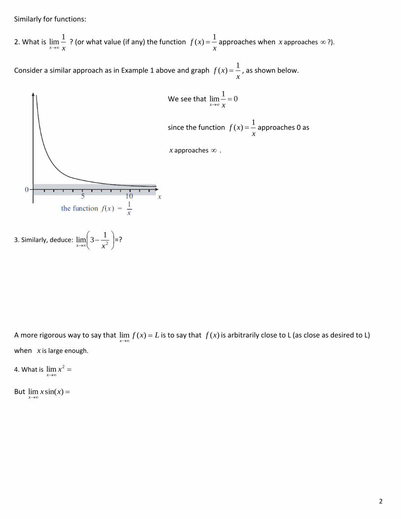
Similarly for functions:

2. What is xx

1lim

? (or what value (if any) the function

xxf

1)( approaches when x approaches ?).

Consider a similar approach as in Example 1 above and graph x

xf1

)( , as shown below.

We see that 01

lim xx

since the function x

xf1

)( approaches 0 as

x approaches .

3. Similarly, deduce:

2

13lim

xx=?

A more rigorous way to say that Lxfx

)(lim is to say that )(xf is arbitrarily close to L (as close as desired to L)

when x is large enough.

4. What is

2lim xx

But

)sin(lim xxx

3

NOTE:

In a more careful approach, in order to convince oneself that Lxfx

)(lim for a specific function )(xf , that is that

)(xf is indeed arbitrarily close to L (as close as desired to L) when x is large enough ,one will often consider a table of

values for increasingly larger values of x to study the behavior of )(xf for those values, consider different challenges

of “closeness” and determine if )(xf satisfies those challenges, or undertake a more rigorous limit

approach. Due to time restrictions, we will not delve into the limit approach in this class, and will usually rely

on the graph of )(xf (and later on algebraic methods) to find )(lim xfx

. We should remember though that

Lxfx

)(lim is to say that )(xf is arbitrarily close to L (as close as desired to L) when x is large enough .

5. Let us now turn to the more general case: )(lim xfax

in which we want to determine the value that )(xf

approaches when x approaches a .

The main difference now is that x approaches a finite value a , and that it can approach this value from the left ax or

from the right ax .

For example, what is 3lim1

xx

? We may well guess (and are correct in saying) that 43lim1

xx

.

This follows easily from a graph of )(xf as shown here (or from our

intuition as well) .

Note that this time we look at both 43lim1

xx

and at

43lim1

xx

, which implies that indeed 43lim1

xx

.

This may not seem very useful , since in this case (as is actually the case for many functions) , if 3)( xxf :

4)1()(lim1

fxfx

. But keep in mind that )(lim xfax

represents actually the value that )(xf approaches when x

approaches a (which in this case agrees with )(af ). There are many instances in which this needs not to be the case,

and calculating the limit is the only way to determine what value )(xf approaches when x approaches a .

For example, calculate:

4

6.

a) 1

1lim

2

1

x

x

x what is )1(f ?

b) x

x

x

)sin(lim

0 what is )0(f ?

c) 2

2

0

39lim

x

x

x

what is )0(f ?

d)

xx

sinlim

0 what is )0(f ?

5

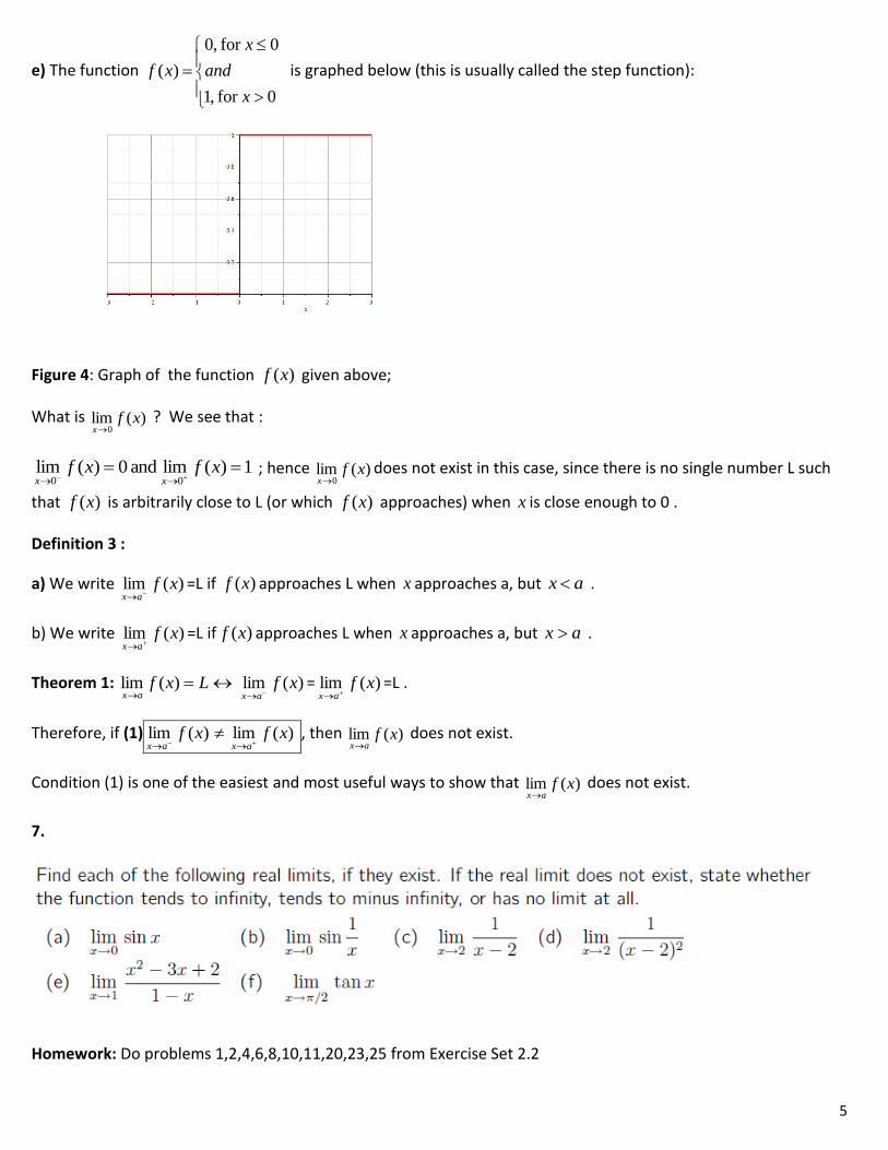
e) The function

0for ,1

0for ,0

)(

x

and

x

xf is graphed below (this is usually called the step function):

Figure 4: Graph of the function )(xf given above;

What is )(lim0

xfx

? We see that :

1)(lim and 0)(lim00

xfxfxx

; hence )(lim0

xfx

does not exist in this case, since there is no single number L such

that )(xf is arbitrarily close to L (or which )(xf approaches) when x is close enough to 0 .

Definition 3 :

a) We write )(lim xfax

=L if )(xf approaches L when x approaches a, but ax .

b) We write )(lim xfax

=L if )(xf approaches L when x approaches a, but ax .

Theorem 1: Lxfax

)(lim )(lim xfax

= )(lim xfax

=L .

Therefore, if (1) )(lim xfax

)(lim xfax

, then )(lim xfax

does not exist.

Condition (1) is one of the easiest and most useful ways to show that )(lim xfax

does not exist.

7.

Homework: Do problems 1,2,4,6,8,10,11,20,23,25 from Exercise Set 2.2

6

2.3. Limit laws. Limits of elementary functions and the squeeze theorem.

A. Limits Laws. Limits of elementary functions:

Goals:

Show an efficient yet rigorous method to calculate limits: show that afxfax

)(lim if )(xf is an

elementary function and if )(af exists .

Solve limits of the form:

0

0 ;

Lesson:

Theorem 1 (Limit Laws):

Consider 212211 and : and : DDaRDgRDf such that MxgLxfaxax

)(lim and )(lim . Then the following

limits exist and are equal to the indicated values:

(1)

even) isn (when 0 and any for L)(lim

any for )(lim

)()(lim

0for )(

)(lim

)()(lim

)()(lim

)()(lim

any for )(lim

LNnxf

NnLxf

MLxgxf

MM

L

xg

xf

MLxgxf

MLxgxf

MLxgxf

RkLkxfk

nn

ax

nn

ax

ax

ax

ax

ax

ax

ax

Proof:

These laws can be shown using the definition 1 in 2.4, and the methods of section 2.4. Some of these proofs are

harder than others, and are shown in Appendix F of the textbook.

From now on, we consider properties (1) true and we use them in problems. Using these, calculate:

Example 1:

a) 32lim 2

5

xx

x b)

1

2lim

2

2

3

x

x

x c)

1

1lim

2

x

x

x

We see that the method to calculate limits ultimately amounts now to substituting )(in with xfax when )(af

exists.

7

We state this clearly in general:

Theorem 2 (substitution):

a) If xPxf n)( is a polynomial of degree n then aPxP nnax

lim .

b) If xQ

xPxf

m

n)( is a rational function (ratio of two polynomials) then

aQ

aP

xQ

xP

m

n

m

n

ax

lim if 0aQm .

c) If )( xf is an algebraic function (a combination of , polynomials and rational functions by using

addition, subtraction, multiplication or composition), then afxfax

)(lim if )(af exists (or, in other

words, if a is in the domain of f(x)) .

Proof: The proof of a) and b) are direct consequences of Theorem 1. The proof of part c) is given in Appendix F in

the textbook (listed as Theorem 8).

Example 2:

Using Theorem 2, calculate the limits:

a) 23

12lim

2

2

x

x

x b) 635lim 23

3

xxx

x .

Do also Example 1 (Page 99, of Section 2.3) in the textbook.

The next theorem will help us solve cases of study of the form

0

0 .

Theorem 3: If )()( xgxf for all Ix , except for Ia , then )(lim)(lim xgxfaxax

.

This theorem allows us to solve limits the form

0

0 , by first algebraically simplifying the function (usually by

cancelling an pax factor from both top and bottom of the fraction) and then calculating the limit of the

simplified function.

Example 3: Using Theorems 3 and 2 above, as well as Theorem 1 in 1.2 calculate the limits:

a) 1

1lim

21

x

x

x b)

h

h

h

9)3(lim

2

0

c)

x

x

x

416lim

2

0

d) If )(lim calculate 4 if 28

4 if 4)(

4xf

xx

xxxf

x

. Then sketch a graph of this function to confirm your result.

e) Calculate xx 0lim

f) Calculate x

x

x 0lim

8

g) 32

132lim

2

2

1

xx

xx

x h)

1

1lim

3

4

1

t

t

t i)

xxxx 20

11lim

j) 32

9lim

2

2

3

xx

x

x k)

xx

xxx

x

2

23

0lim l)

23

1

2

2lim

22 xxxxx

m) x

xx

x

33lim

0 n)

24

11lim

0

x

x

x

B. The squeeze theorem:

New types of limits (including limits of trigonometric functions and combinations of these) can be calculated using

an inequality result involving limits called the squeeze theorem.

This theorem is based on:

Theorem 4: If )()( xgxf when x is near a (except possibly at a ) and MxgLxfaxax

)(lim and )(lim , then :

(2) ML .

Proof: See the proof of Theorem 2 in Appendix F.

Based on this theorem, we can easily prove the following:

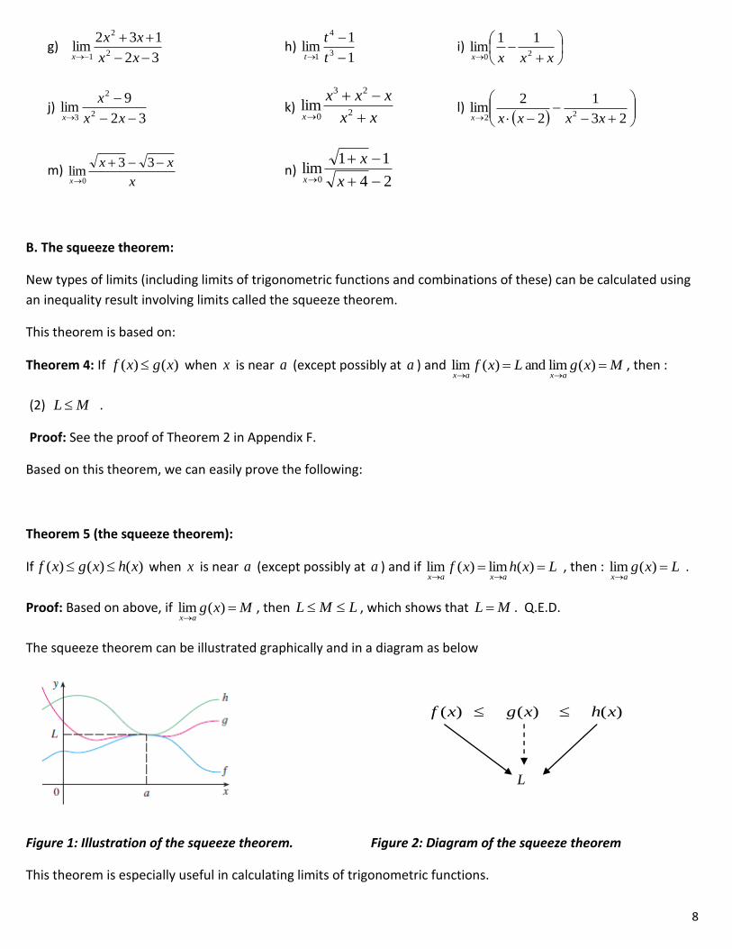
Theorem 5 (the squeeze theorem):

If )()()( xhxgxf when x is near a (except possibly at a ) and if )(lim)(lim Lxhxfaxax

, then : )(lim Lxgax

.

Proof: Based on above, if Mxgax

)(lim , then LML , which shows that ML . Q.E.D.

The squeeze theorem can be illustrated graphically and in a diagram as below

)( )( )( xhxgxf

L

Figure 1: Illustration of the squeeze theorem. Figure 2: Diagram of the squeeze theorem

This theorem is especially useful in calculating limits of trigonometric functions.

9

First, based on it, we can prove:

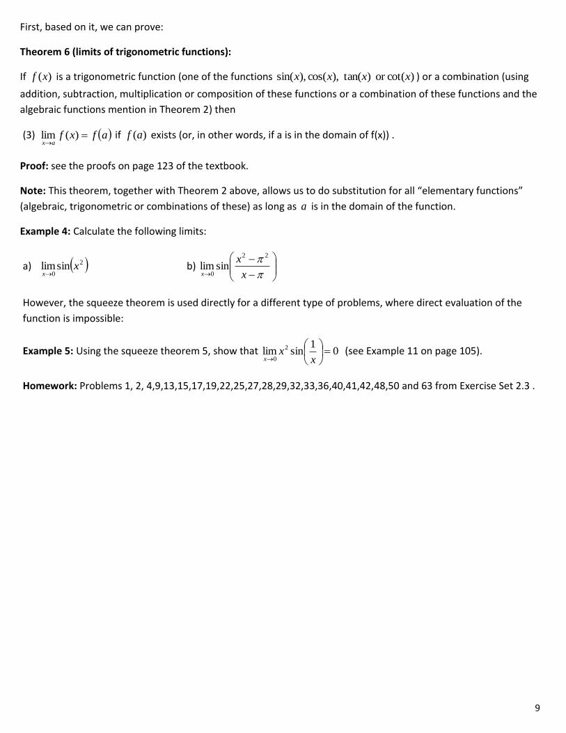
Theorem 6 (limits of trigonometric functions):

If )(xf is a trigonometric function (one of the functions )cot(or )tan( ),cos( ),sin( xxxx ) or a combination (using

addition, subtraction, multiplication or composition of these functions or a combination of these functions and the

algebraic functions mention in Theorem 2) then

(3) afxfax

)(lim if )(af exists (or, in other words, if a is in the domain of f(x)) .

Proof: see the proofs on page 123 of the textbook.

Note: This theorem, together with Theorem 2 above, allows us to do substitution for all “elementary functions”

(algebraic, trigonometric or combinations of these) as long as a is in the domain of the function.

Example 4: Calculate the following limits:

a) 2

0sinlim x

x b)

x

x

x

22

0sinlim

However, the squeeze theorem is used directly for a different type of problems, where direct evaluation of the

function is impossible:

Example 5: Using the squeeze theorem 5, show that 01

sinlim 2

0

xx

x (see Example 11 on page 105).

Homework: Problems 1, 2, 4,9,13,15,17,19,22,25,27,28,29,32,33,36,40,41,42,48,50 and 63 from Exercise Set 2.3 .

10

2.6. Limits at infinity and infinite limits:

In section 2.3 we were able to calculate afxfax

)(lim if a is in the domain of )(xf , or for a case of study of the

form

0

0.

In this section we will study new important types of limits involving .

A. Infinite limits:

Definition 1:

a)

)(lim xfax

if the values of )(xf can be made arbitrarily large when x is close enough to a .

b)

)(lim xfax

if the values of )(xf can be made arbitrarily large negative when x is close enough to a .

Example 1:

a) Graph 2

1)( and

1)(

xxg

xxf and infer infinite limit results from the graph.

b) Using the definition above, show that

1

lim and 1

lim , 1

lim ,1

lim00

2020

xxxx xxxx

c) What is

xx

1lim

0 ?

Note: We generalize the results from the example above and state:

(1) 0

1 and

0

1 . These two results mean that

0)(lim if

)(

1lim xf

xf axax

and

0)(lim if

)(

1lim xf

xf axax (of course, in these results a could be replaced by aa or , as

needed).

Also

0)(lim xf

ax means that as x approaches a, f(x) approaches 0 but only with positive values (f(x) is positive as

x approaches a), and

0)(lim xf

ax means that as x approaches a, f(x) approaches 0 but only with negative values

(f(x) is negative as x approaches a) .

The result (1) is the most important tool to calculate infinite limits. Therefore, in order to evaluate a limit of the

form

0

1, we evaluate the function, and determine the sign of the denominator (best by using a sign table for it

!!), then use (1).

11

Example 2:

Calculate the limits:

a) 3

2lim

3 x

x

x and

3

2lim

3 x

x

x , therefore ?

3

2lim

3

x

x

x

b) 23 3

2lim

x

x

x

c) )tan(lim

2

xx

and )tan(lim

2

xx

, therefore ?)tan(lim

2

xx

d) Do problems 29, 31 and 35 from Exercise Set 2.2 in the textbook.

In the previous examples, if )(or )(lim

xfax

, or if )(or )(lim

xfax

or if )(or )(lim

xfax

, then

the line ax is called a Vertical Asymptote (V.A.) for the graph of )(xf (see, for example, the limits in Example 1).

Therefore:

Definition 2: The line ax is called a Vertical Asymptote (V.A.) for the graph of )(xf if at least one of the

following six cases takes place:

)(or )(lim

xfax

, or )(or )(lim

xfax

or )(or )(lim

xfax

.

Practically, to calculate the V.A. for a given function, we calculate first the zeros of the denominator (if the function

is a fraction) and then calculate the limit of the function at these points.

Example 3:

a) Problem 38 from problem set 2.2 in the textbook.

b) Find all the vertical asymptotes of :

i) 95

8)(

xxxf ii)

4310

7)(

x

xxf

iii)

x

xxf

)cos()(

iv) x

xxf

cos)( v)

x

xxf

)sin()( vi)

x

xxf

2sin

)tan()(

B. Limits at infinity:

We turn now to the (last main) case when x .

Definition 3:

a) Lxfx

)(lim if )(xf is arbitrarily close to L when x is large enough. Also:

b) Lxfx

)(lim if )(xf is arbitrarily close to L when x is large enough and negative.

c) Definition 1 can be combined with Definition 3 (Exercise) to produce:

)(or )(lim and )(or )(lim

xfxfxx

.

12

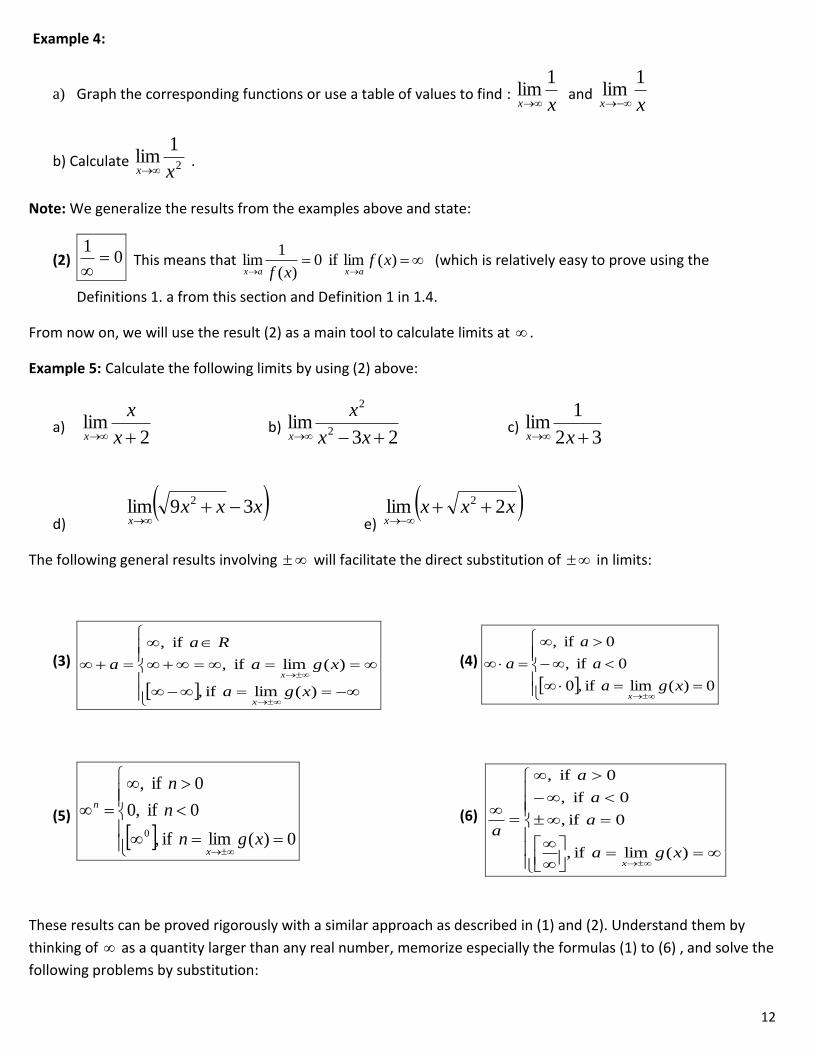
Example 4:

a) Graph the corresponding functions or use a table of values to find : xx

1lim

and

xx

1lim

b) Calculate 2

1lim

xx .

Note: We generalize the results from the examples above and state:

(2) 01

This means that

)(lim if 0

)(

1lim xf

xf axax (which is relatively easy to prove using the

Definitions 1. a from this section and Definition 1 in 1.4.

From now on, we will use the result (2) as a main tool to calculate limits at .

Example 5: Calculate the following limits by using (2) above:

a) 2

lim x

x

x b)

23lim

2

2

xx

x

x c)

32

1lim

xx

d) xxx

x39lim 2

e) xxx

x2lim 2

The following general results involving will facilitate the direct substitution of in limits:

(3)

)(lim if ,

)(lim if ,

if ,

xga

xga

Ra

a

x

x

(4)

0)(lim if ,0

0 if ,

0 if ,

xga

a

a

a

x

(5)

0)(lim if ,

0 if ,0

0 if ,

0 xgn

n

n

x

n

(6)

)(lim if ,

0 if ,

0 if ,

0 if ,

xga

a

a

a

a

x

These results can be proved rigorously with a similar approach as described in (1) and (2). Understand them by

thinking of as a quantity larger than any real number, memorize especially the formulas (1) to (6) , and solve the

following problems by substitution:

13

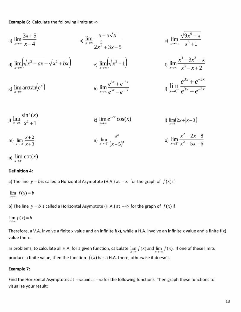
Example 6: Calculate the following limits at :

a) 4

53lim

x

x

x b)

532

lim

2

3

xx

xxx

x c)

1

9lim

3

6

x

xx

x

d) bxxaxxx

22lim e) 1lim 2

xx

f) 2

3lim

3

24

xx

xxx

x

g) x

xearctanlim

h) xx

xx

x ee

ee33

33

lim

i) xx

xx

x ee

ee33

33

0lim

j) 1

)(sinlim

2

2

x

x

x k) )cos(lim 2 xe x

x

l) 32lim

3

xx

x

m) 3

2lim

3

x

x

x n)

35 5lim

x

e x

x o)

65

82lim

2

2

2

xx

xx

x

p) )cot(lim xx

Definition 4:

a) The line by is called a Horizontal Asymptote (H.A.) at for the graph of )(xf if

bxfx

)(lim

b) The line by is called a Horizontal Asymptote (H.A.) at for the graph of )(xf if

bxfx

)(lim

Therefore, a V.A. involve a finite x value and an infinite f(x), while a H.A. involve an infinite x value and a finite f(x)

value there.

In problems, to calculate all H.A. for a given function, calculate )(lim and )(lim xfxfxx

. If one of these limits

produce a finite value, then the function )(xf has a H.A. there, otherwise it doesn’t.

Example 7:

Find the Horizontal Asymptotes at at and for the following functions. Then graph these functions to

visualize your result:

14

a) 1

1)(

2

2

x

xxf b)

2

12)(

2

2

xx

xxxf c)

56)(

2

3

xx

xxxf

Homework:

What problems are left from above, and problems 19, 21,22,38,41,44 and 45 from the Exercise Set 2.6 in the

textbook.

2.5 Continuity of functions:

Functions which have the property that )()(lim afxfax

are called continuous at a . Continuity of functions is a

very important property which some functions verify on an entire interval or on their entire domain of definition.

Functions which are continuous on an interval will satisfy other theorems (such as the intermediate value

theorem) which allows us to find their zeros.

In this section we will learn tools (definitions and theorems) to establish the continuity of functions at a point and

on an entire interval, as well as the intermediate value theorem for continuous functions.

Definition 1: A function RDf : is continuous at a number Da if (1) )()(lim afxfax

.

Note that (1) actually says 3 things about the function )(xf . It says that:

a) )(af exists ( )(xf is defined at a ) ;

b) )(lim xfax

exists and

c) )()(lim afxfax

.

Remembering the meaning of )(lim xfax

, we realize that (1) represents the intuitive fact that )(xf does not have a

jump (or a break – discontinuity) at a . Therefore, when we trace the graph of )(xf close to a , the graph passes

continuously through the point )(, afa .

Example 1: See Example 1 on page 119 in the textbook.

Example 2: Determine the continuity of the following functions at the indicated point:

a) 2

2)(

2

x

xxxf at 2a b) 0at

0for 1

0 if )(

2

a

x

xxxf

c) 0at

0for 0

0 if )(

a

x

xx

x

xf . Then graph these functions to visualize your claim.

Note that some functions (such as xxf )( ) are not defined to the left of 0a , and therefore only a side

continuity can be defined there. Side continuity is also useful to define continuity on an entire interval.

15

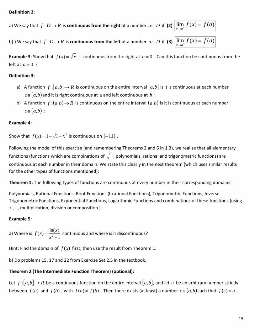
Definition 2:

a) We say that RDf : is continuous from the right at a number Da if (2) )()(lim afxfax

b) ) We say that RDf : is continuous from the left at a number Da if (3) )()(lim afxfax

Example 3: Show that xxf )( is continuous from the right at 0a . Can this function be continuous from the

left at 0a ?

Definition 3:

a) A function Rbaf ,: is continuous on the entire interval ba, is it is continuous at each number

bac , and it is right continuous at a and left continuous at b ;

b) A function Rbaf ,: is continuous on the entire interval ba, is it is continuous at each number

bac , ;

Example 4:

Show that 211)( xxf is continuous on 1,1 .

Following the model of this exercise (and remembering Theorems 2 and 6 in 1.3), we realize that all elementary

functions (functions which are combinations of , polynomials, rational and trigonometric functions) are

continuous at each number in their domain. We state this clearly in the next theorem (which uses similar results

for the other types of functions mentioned):

Theorem 1: The following types of functions are continuous at every number in their corresponding domains:

Polynomials, Rational Functions, Root Functions (Irrational Functions), Trigonometric Functions, Inverse

Trigonometric Functions, Exponential Functions, Logarithmic Functions and combinations of these functions (using

+ , - , multiplication, division or composition ).

Example 5:

a) Where is 1

)ln()(

2

x

xxf continuous and where is it discontinuous?

Hint: Find the domain of )(xf first, then use the result from Theorem 1.

b) Do problems 15, 17 and 22 from Exercise Set 2.5 in the textbook.

Theorem 2 (The Intermediate Function Theorem) (optional):

Let Rbaf ,: be a continuous function on the entire interval ba, , and let u be an arbitrary number strictly

between )(af and )(bf , with )()( bfaf . Then there exists (at least) a number bac , such that ucf )( .

16

Note: What Theorem 2 suggests is that continuous functions achieve (with a particular )(cf ) all values in their

range (if their range is an interval) . The proof of this theorem can be found in more advanced Calculus texts, and it

is based on Cauchy’s completion axiom (see a model of the proof on Wikipedia).

We Use Theorem 2 to find zeros of a continuous function, or to prove that such zeros exist.

Example 6:

Show that there is a root of the equation 02364 23 xxx between 1 and 2. Can we reduce the length of the

interval which contains this root? Can you suggest an algorithm to find the root to a desired precision?

Homework:

What left from above and problems 3,4,5,6,7, 16, 18, 19, 20, 21,4042,45,46,51 and 54.

2.7 Review:

In this chapter, we learnt

- The notion Lxfax

)(lim at an intuitive level (Definition 1, how to use graphs and tables to determine

limits: Section 2.2) ;

- The rigorous notion of Lxfax

)(lim (Definition 2 and 3 (the definition): Section 2.4);

- Practical methods to calculate limits: substitution and cases of study, infinite limits and limits at infinity

(Sections 2.3 and 2.6)

- Continuity of functions based on limits (Section 2.5) .

Learn the main results from each section (definitions, theorems and formulas) (best by writing a brief review guide

which include these) , then solve the following problems:

- In the textbook, do the Review problems from pages 165 to 168, with the exception of the problems

involving the derivative of a function or rates of change (problems 11,12,13,14 from Concept Check,

problems 19,20,21 from True or False, and problems 38 to 50 from Exercises).

- Do the problems below:

1. Calculate xx

coslim5.0

by building a table of values xx cos, around 0.5 (the intuitive approach of guessing

the limit using a table (used in 1.2) ).

2. Calculate the following limits (using methods from the sections 2.3 and 2.6):

a) 5

56lim

2

5

x

xx

x b)

43

4lim

2

2

1

xx

xx

x c)

h

h

h

8)2(lim

3

0

d) 1

1lim

3

4

1

x

x

x e)

8

2lim

32

x

x

x f)

xxxx 20

11lim

17

g) x

xx

x

11lim

0 h)

20 16

4lim

xx

x

x

i)

x

x

x

11

0

3)3(lim

j) 1

1lim

3

2

xx

x

x k)

12

23lim

x

x

x l)

542

264lim

3

23

xx

xx

x

m) 1

9lim

3

6

x

xx

x n)

1

9lim

3

6

x

xx

x o) xxx

x39lim 2