chapter 2 introduction to brain anatomy, glioma and magnetic resonance ...shodhganga.inflibnet.ac.in...

19

Chapter 2

Introduction to Brain Anatomy, Glioma and Magnetic Resonance imaging

Techniques

The purpose of this chapter is to introduce some basic idea about brain anatomy, different types of tumor present in the brain and different imaging techniques adopted to visualize the complex brain structures. It also discusses the different grades of glioma tumors, its causes and symptoms. It introduces types of magnetic resonance imaging techniques adopted for visualizing complex brain structures, to find out various brain disorders and for diagnosing brain tumors. Additional topic discussed in this chapter gives a brief idea about advanced magnetic resonance imaging techniques. Glioma tumors, different types of noise, partial volume effect and intensity in-homogeneities present in Magnetic Resonance Images are also presented.

Chapter 2

20

Introduction to Brain Anatomy, Glioma and Magnetic Resonance imaging Techniques

21

2.1 Anatomy of the brain Human brain is the most valuable, interesting and amazing part of our

body. The brain acts as the control centre of the central nervous system and gives us the ability to learn and understand. The brain controls and coordinates most sensory systems, movement, behaviour, and homeostatic body functions such as heart rate, blood pressure, fluid balance, and body temperature. The brain is the source of cognition, emotion, memory, and motor, and other forms of learning. Much behaviour such as simple reflexes and basic locomotion, can be executed under spinal cord control alone.

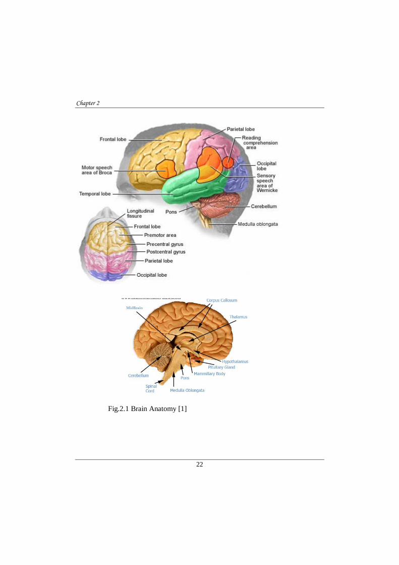
The human brain is made up of four main parts: the cerebral cortex, the cerebellum, the brain stem, and the meninges as shown in Fig.2.1

The cerebral cortex is the largest part of the brain, is associated with conscious thought, movement and sensation. It contains two cerebral hemispheres each controlling the opposite side of the body. The two halves are connected by the corpus callosum, a bridge of wide, flat neural fibers that act as communication relays between the two sides and is divided into four lobes such as : the frontal, temporal, parietal, and occipital lobes. The main functions of the four lobes are as follows:

Frontal Lobe is one of the four lobes of the cerebral hemisphere which extending from behind the forehead back to the parietal lobe, is the brain region that separates humans from our primate cousins. It controls attention, behavior, abstract thinking, problem solving, creative thought, emotion, intellect, initiative, judgment, coordinated movements, muscle movements, smell, physical reactions, and personality. Parietal Lobe houses the sensory cortex and motor cortex which plays an important role in controlling tactile sensation, response to internal stimuli, sensory comprehension, language reading, and some visual functions. Sensory cortex is located in the front part of the parietal lobe, or in other words, the middle area of the brain. The sensory cortex receives information from the spinal cord about the sense of touch, pressure, pain, and the perception of the position of body parts and their movements. Motor cortex is the area located in the middle, top part of the brain that helps control movement in various parts of the body.

Chapter 2

22

Fig.2.1 Brain Anatomy [1]


23

Occipital Lobe located at the back of the brain, is the seat of the primary visual cortex, the brain region responsible for processing and interpreting visual information. Broca's Area is located in the opercular and triangular sections of the inferior frontal gyrus. The function of this area is the understanding of language, speech, and the control of facial neurons.

Temporal lobe reaching from the temple back towards the occipital lobe, the temporal lobe is a major processing center for language and memory. It controls auditory and visual memories, language, some hearing and speech, language, plus some behavior. Wernicke's area is part of the temporal lobe that surrounds the auditory cortex and is thought to be essential for understanding and formulating speech. Damage in Wernicke's area causes deficits in understanding spoken language.

Cerebellum is located at the lower back of the head and is connected to the brain stem. It is the second largest structure of the brain. The cerebellum controls complex motor functions such as walking, balance, posture, and general motor coordination.

The brain stem The brain stem is involved with autonomic control of processes like breathing and heart rate as well as conduction of information to and from the peripheral nervous system, the nerves and ganglia found outside the brain and spinal cord which includes the Medulla oblongata, Pons, and Midbrain. This is located at the bottom of the brain and connects the cerebrum to the spinal cord. The brain stem controls many vitally important functions including motor and sensory pathways, cardiac and respiratory functions, and reflexes.

The meninges. These are the membranes that surround and protect the brain and spinal cord. There are three meningeal layers, called the dura mater, arachnoid, and pia mater. The cerebrospinal fluid (CSF) is produced near the center of the brain, in the lateral ventricles, and circulates around the brain and spinal cord between the arachnoid and pia layers.

Cerebrospinal Fluid, also called CSF, is a clear substance that circulates through the brain and spinal cord. It provides nutrients and serves to cushion the brain and therefore protect it from injury. As this fluid gets absorbed, more is produced from the choroid plexus, a structure located in the ventricles. A brain

Chapter 2

24

tumor can cause a build-up or blockage of CSF. Ventricles of the brain are connected cavities within the brain, where cerebrospinal fluid is produced.

Hypothalamus is a region of the brain in partnership with the pituitary gland that controls the hormonal processes of the body as well as temperature, mood, hunger, and thirst. Optic Chiasm is located beneath the hypothalamus and is where the optic nerve crosses over to the opposite side of the brain. Pineal Gland controls the response to light and dark. The exact role of the pineal gland is not certain.

Pituitary Gland is a small, bean-sized organ that is located at the base of the brain and is connected to the hypothalamus by a stalk. The pituitary gland secretes many essential hormones for growth and sexual maturation. Thalamus is located near the center of the brain and controls input and output to and from the brain, as well as the sensation of pain and attention. [1-3]

Neurons, or brain cells, are made up of cell bodies, axons, and dendrites. The cells mainly connect to one another through synapses (small junctions between brain cells where neurotransmitters and other neuro-chemicals are passed). Synapses are often found between the axons and dendrites, which allows the cells to signal to one another. Current estimates suggest the brain has approximately 86 billion neurons [3]. The brain is made up of two types of matter: gray and white. Gray matter consists of the cell bodies and dendrites of the neurons, as well as supporting cells called astroglia and oligodendrocytes. White matter, however, is made up of mostly of axons sheathed in myelin, an insulating-type material that helps cells propagate signals more quickly. It’s the myelin that gives the white matter its lighter color. For many years; neuroscientists believed white matter was simply a support resource for gray matter. However, recent studies show that white matter architecture is important in processes like learning and memory [4]

2.2 Types of brain tumors When most normal cells grow old or get damaged, they die, and new cells

take their place. Sometimes, this process goes wrong. New cells form when the body doesn't need them, and old or damaged cells don't die as they should. The buildup of extra cells often forms a mass of tissue called a growth or tumor. Brain


25

tumors are composed of cells that exhibit unrestrained growth in the brain. They can be benign (noncancerous, meaning that they do not spread elsewhere or invade surrounding tissue) or malignant (cancerous).The brain and spinal column make up the central nervous system (CNS), where all vital functions, including thought, speech, and strength of the body are controlled. When a tumor arises in the CNS, it is especially problematic because of the potential effect on a person's thought processes and movements [3].

The brain tumors are broadly classified into primary and secondary (metastatic) tumors. The terms primary and metastatic describe where the tumor has originated and brain tumors are generally classified as one or the other. Primary brain tumors arise from the brain or spinal cord while metastatic brain tumors arise from other tissue and have spread to the brain. This is the most basic form of classifying brain tumors, but yields great insight into the characteristics of these complex growths and how they might be treated.

The following section describes about primary and secondary brain tumors.

2.2.1 Secondary (Metastatic) Malignant Brain Tumors A secondary brain tumor is a cancerous tumor that started in another part

of the body (such as the breast, lung, or colon) and then spread to the brain. Secondary tumors are about three times more common than primary tumors of the brain [7,8]. Many types of cancer can spread (metastasize) to the brain, but melanoma, breast, lung, and kidney cancer are among the most common. Cancer cells are spread by blood or lymphatic vessels. Metastatic brain tumors are more common than primary brain tumors. It is believed that the commonality is not because cancer types are becoming more aggressive, it is just that people are living longer from their cancer types, and this time allows for metastasis to occur. Usually, multiple tumors develop. Solitary metastatized brain cancers may occur but are less common. Metastatic or secondary tumors of the brain will occur in 20% to 40% of patients with cancer.

2.2.2 Primary Brain Tumors There are more than 100 types of primary brain tumors. Primary tumors

start in the brain, whereas secondary tumors spread to the brain from another site

Chapter 2

26

such as the breast or lung. There are many types and subtypes of primary brain tumors. They include gliomas (which in turn include astrocytomas, oligodendrogliomas, and ependydomas), meningomas, medullablastomas, pituitary adenomas, and central nervous system lymphomas [9].

Benign Brain Tumors. Benign tumors represent half of all primary brain tumors. Their cells look relatively normal, grow slowly, and do not spread (metastasize) to other sites in the body or invade brain tissue. Benign tumors can still be serious and even life-threatening if they are in vital areas of the brain where they exert pressure on sensitive nerve tissue or if they increase pressure within the brain. While some benign brain tumors may pose a health risk, including risk of disability and death, most are usually successfully treated with techniques such as surgery [4].

Malignant Brain Tumors. A primary malignant brain tumor is one that originates in the brain itself. Although primary malignant brain tumors often shed cancerous cells to other sites in the central nervous system (the brain or spine), they rarely spread to other parts of the body. Brain tumors are generally named and classified according to the type of brain cells from which they originate and the

Fig 2.2. Primary Brain tumor


27

location in which the cancer develops. Malignant brain tumors are further classified using a grade: low, intermediate, or high. More information can be found in Staging/Grading [4-6].The biologic diversity of these tumors, however, makes classification difficult.

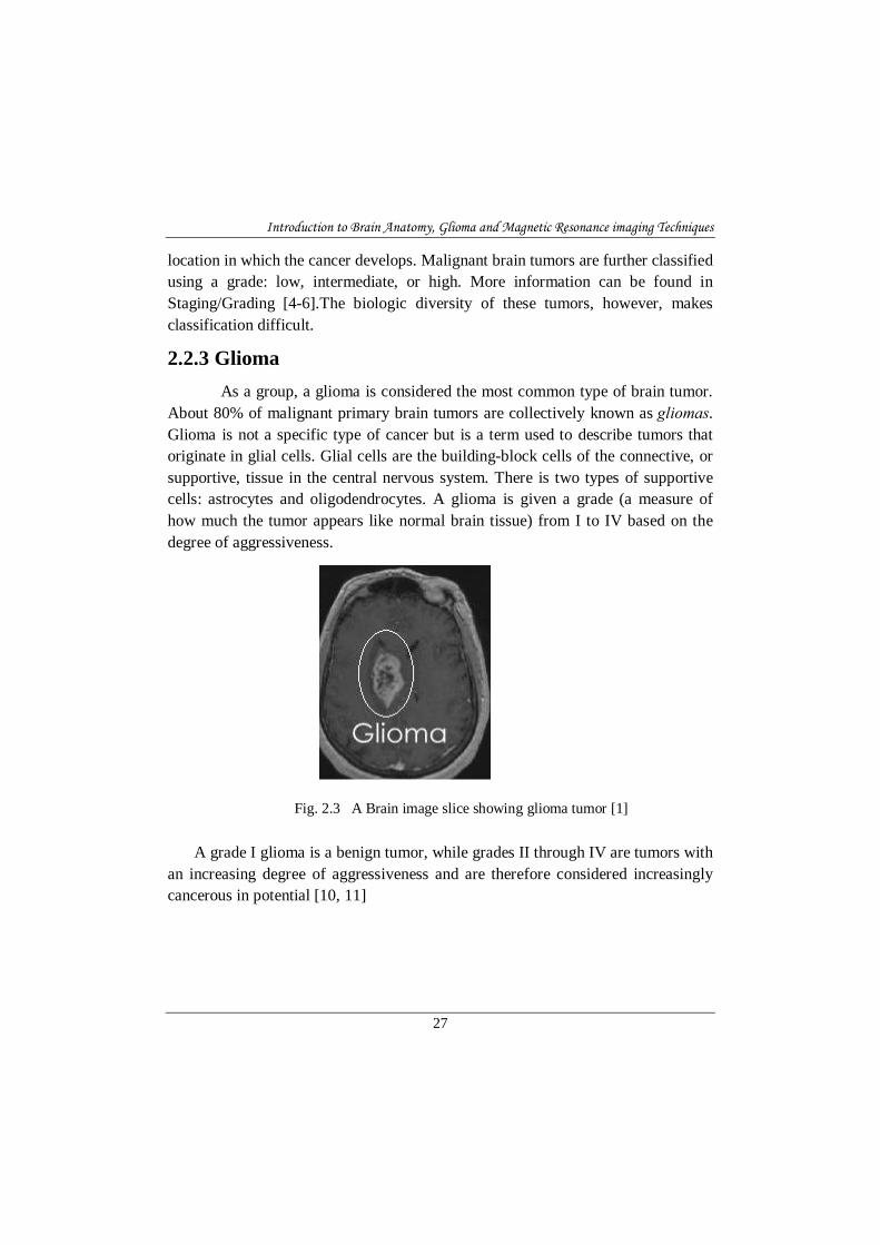
2.2.3 Glioma As a group, a glioma is considered the most common type of brain tumor.

About 80% of malignant primary brain tumors are collectively known as gliomas. Glioma is not a specific type of cancer but is a term used to describe tumors that originate in glial cells. Glial cells are the building-block cells of the connective, or supportive, tissue in the central nervous system. There is two types of supportive cells: astrocytes and oligodendrocytes. A glioma is given a grade (a measure of how much the tumor appears like normal brain tissue) from I to IV based on the degree of aggressiveness.

A grade I glioma is a benign tumor, while grades II through IV are tumors with

an increasing degree of aggressiveness and are therefore considered increasingly cancerous in potential [10, 11]

Fig. 2.3 A Brain image slice showing glioma tumor [1]

Chapter 2

28

Grades I and II are considered low-grade and grades III and IV are considered high-grade. Grades I and II are the slowest-growing and least malignant; grade II tumors are generally considered borderline between benign and malignant. Grade III tumors are considered malignant and grow at a moderate rate. Grade IV tumors, such as glioblastoma multiforme, are the fastest-growing and most malignant primary brain tumor [12].High-grade gliomas are highly-vascular and have a tendency to infiltrate. Often tumor growth causes a breakdown of the blood–brain barrier in the vicinity of the tumor. As a rule, high-grade gliomas almost always grow back even after complete surgical excision, and so are commonly called recurrent cancer of the brain.

On the other hand, low-grade gliomas grow slowly, often over many years, and can be followed without treatment unless they grow and cause symptoms. Several acquired (not inherited) genetic mutations have been found in gliomas. There are several glial cell types from which gliomas form. Most common subtype of gliomas are called either astrocytoma or oligodendroglioma, or a mixture of both.

Astrocytomas are primary brain tumors derived from astrocytes, which are star-shaped glial cells. Astrocytomas account for about 60% of all malignant

Fig. 2.4 An MRI of a patient with two separate types of brain tumor, a low grade glioma in the right frontal lobe (which is very difficult to see) and a high grade glioma (Glioblastoma) in the right parietal lobe which shows more (gray white appearance) contrast enhancement [1]


29

primary brain tumors. It is the most common type of glioma and begins in cells called astrocytes in the cerebrum or cerebellum. There are four grades of astrocytoma[12]. Astrocytomas are the most common of the primary brain tumors. The pathologist, using a microscope, grades these tumors on a scale of I to IV based on how quickly the cells are reproducing, as well as their potential to invade nearby tissue [12].

Astrocytoma tumor types by grade include:

• Grade I. Pilocytic astrocytoma is one of the most common types of glioma in children.It is a slow-growing tumor that is most often benign and rarely spreads into nearby tissue. It accounts for about 2% of all brain tumors.

• Grade II. Diffuse astrocytoma (also called low-grade astrocytoma) is a slow-growing tumor that can often spread into nearby tissue and can become a higher grade. It accounts for about 11% of all brain tumors, typically occurring in men and women of ages 20 – 60. Grades I and II astrocytomas are the slowest growing tumors, and are also called low-grade astrocytomas.

• Grade III. Anaplastic astrocytoma is a malignant tumor that can quickly grow and spread to nearby tissues. It accounts for about 3% of all brain tumors. It typically occurs in adults of ages 30 - 60 and is more common among men than women.

• Grade IV. Glioblastoma multiforme (GBM), also called glioblastoma, accounts for about 50% of all astrocytomas and about 20% of all brain tumors.It is one of the deadliest types of brain tumors. These highly malignant, aggressive and complex tumors grow rapidly. They are most common in older adults (50s - 70s), particularly men. Only about 10% of childhood brain tumors are glioblastomas. It also is the most resistant to current standard treatment – surgery, followed by radiation and chemotherapy [3].

Chapter 2

30

2.2.3.1 Statistics

It is estimated that about 52,000 people are diagnosed with a primary brain tumor (benign or malignant) each year. In 2012, an estimated 22,070 adults (12,010 men and 10,060 women) in the United States were diagnosed with primary malignant tumors of the brain and spinal cord. It is estimated that 12,920 deaths (7,330 men and 5,590 women) from this disease will occur this year. Brain tumors are the tenth most common cause of cancer death in women [13]. Primary malignant brain tumors account for about 2% of all cancers. However, brain and spinal cord tumors are the second most common type of cancer in children (after leukemia).

Survival statistics should be interpreted with caution. Estimates are based on data from thousands of cases of glioma tumors in the United States each year, but the actual risk for a particular individual may differ. It is not possible to tell a person how long he or she will live with a glioma tumor. Because the survival statistics are measured in five-year (or sometimes one-year) intervals, they may not represent advances made in the treatment or diagnosis of this cancer. In general, brain tumors are slightly more likely to occur in men than in women. Some specific types of brain tumors, such as meningiomas, are more common in women. Most brain tumors in adults occur between the ages of 65 - 79. Brain tumors also tend to occur in children younger than the ages of 8. In children, glioblastomas are the leading cause of death from solid tumors.

2.2.3.2 Prognosis and Survival rates

Recent advances in surgical and radiation treatments have significantly extended average survival rates and can also reduce the size and progression of malignant glioma [15].

The survival rates in people with brain tumors depend on many different variables:

• Type of tumor (such as astrocytoma, oligodendroglioma, or ependymoma) • Location and size of tumor (these factors affect whether or not the tumor

can be surgically removed) • Tumor grade • Patient's age


31

• Patient's ability to function • How far the tumor has spread

Survival rates tend to be highest for younger patients and decrease with age. Five-year survival rates range from 66% for children ages 0 - 19 years, to 5% for adults of age of 75 years and older. Glioblastoma multiforme has the worst prognosis with 5-year survival rates of only 13% for people of ages 20 - 44, and 1% for patients age 55 – 64 [17, 18].

2.2.3.3 Diagnosis

Diagnosis of brain tumors involves a neurological examination and various types of imaging tests. Imaging techniques include magnetic resonance imaging (MRI), computed tomography (CT), and positron emission tomography (PET) scan. Biopsies may be performed as part of surgery to remove a tumor, or as a separate diagnostic procedure.

2.2.3.4 Treatment

The standard approach for treating brain tumors is to reduce the tumor as much as possible using surgery, radiation treatment, or chemotherapy. Such treatments are typically used in combination with each other [19].

2.3 Imaging Techniques Among the modern medical imaging technologies, Positron Emission

Tomography (PET) and Magnetic Resonance Imaging (MRI) are considered to be the most powerful diagnostic inventions. In the 1940s, modern medical imaging technology began with advancements in nuclear medicine. Advanced imaging techniques have dramatically improved the diagnosis of brain tumors.

Magnetic Resonance Imaging. Magnetic resonance imaging (MRI) is the standard crucial step for diagnosing a brain tumor. It provides pictures from various angles that can help doctors to construct a three-dimensional image of the tumor. It gives a clear picture of tumors near bones, smaller tumors, brain stem tumors, and low-grade tumors. MRI is also useful during surgery to show tumor bulk, for accurately mapping the brain, and for detecting response to therapy. Its details are given in next section 2.3.1

Chapter 2

32

Computed Tomography. In the early 1970s, by combining the diagnostic properties of X-rays with computer technology, scientists were able to construct 3D images of the human body in vivo for the first time, prompting the birth of the Computed Tomography (CT). The emergence of CT was an important event that motivated scientists to invent PET and MRI [20 ].Computed tomography (CT) uses a sophisticated X-ray machine and a computer to create a detailed picture of the body's tissues and structures. It is not as sensitive as an MRI in detecting small tumors, brain stem tumors, and low-grade tumors. But it is useful for finding bone disorders. Often, doctors will inject the patient with a contrast material to make it easier to see abnormal tissues. A CT scan helps locate the tumor and can sometimes help determine its type. It can also help detect swelling, bleeding, and associated conditions. In addition, computed tomography is used to evaluate the effectiveness of treatments and watch for tumor recurrence [20].

Positron Emission Tomography. Positron emission tomography (PET) provides a picture of the brain's activity rather than its structure by tracking sugar that has been labeled, with a radioactive tracer. It is sometimes able to distinguish between recurrent tumor cells and dead cells or scar tissue caused by radiation therapy. PET is not routinely used for diagnosis, but it may supplement MRIs to help determine tumor grade after a diagnosis. Data from PET may also help improve the accuracy of newer radiosurgery techniques. PET scans are often done along with a CT scan.

Other Imaging Techniques. Numerous other advanced or investigational imaging techniques available include:

• Single photon emission tomography (SPECT) is similar to PET but is not as effective in distinguishing tumor cells from destroyed tissue after treatments. It may be used after CT or MRI to help distinguish between low-grade and high-grade tumors [21].

• Magnetoencephalography (MEG) scans measure the magnetic fields created by nerve cells as they produce electrical currents. It is used to evaluate functioning of various parts of the brain. However, this procedure is not widely available [21].


33

• MRI angiography evaluates blood flow. MRI angiography is usually limited to planning surgical removal of a tumor suspected of having a large blood supply.

Lumbar Puncture (Spinal Tap): A lumbar puncture is used to obtain a sample of cerebrospinal fluid, which is examined for the presence of tumor cells. Spinal fluid may also be examined for the presence of certain tumor markers (substances that indicate the presence of a tumor). However, most primary brain tumors do not currently have identified tumor markers. A computed tomography (CT) scan or magnetic resonance imaging (MRI) should generally be performed before a lumbar procedure to make sure that the procedure can be performed safely.

Biopsy: A biopsy is a surgical procedure in which a small sample of tissue is taken from the suspected tumor and examined under a microscope for malignancy. The results of the biopsy also provide information on the cancer cell type. Biopsies may be performed as part of surgery to remove a tumor, or as a separate diagnostic procedure. With some very slow-growing cancers, such as those that occur in the midbrain or optic nerve pathway, patients may be closely observed and not treated until the tumor shows signs of growth. The diagnosis and detection of glioma currently rely on the histopathologic examination of biopsy specimens, but variations in tissue sampling for these heterogeneous tumors and restrictions on surgical accessibility make it difficult to be sure that the samples obtained are representative of the entire tumor.

2.3.1 Magnetic Resonance Imaging Basic Principles.

Magnetic resonance imaging (MRI) is a medical imaging technique used in radiology to visualize detailed internal structures. MRI makes use of the property of nuclear magnetic resonance (NMR) to image nuclei of atoms inside the body. MRI imaging techniques are broadly classified into two types : Conventional and advanced magnetic resonance imaging techniques. MR imaging is the preferred technique for the diagnosis, treatment planning, and monitoring of patients with neoplastic Central Nervous System lesions. Conventional MR imaging, with gadolinium-based contrast enhancement, is increasingly combined with advanced,

Chapter 2

34

functional MR imaging techniques to offer morphologic, metabolic, and physiologic information [22 ].

An MRI creates a three dimensional picture of the brain, which allows

doctors to more precisely locate problems such as tumors. An MRI machine (Fig.2.5) uses a powerful magnetic field to align the magnetization of protons in the hydrogen atom present in the body, and radio frequency fields to systematically alter the alignment of this magnetization. This causes the protons to produce a rotating magnetic field of larger frequency detectable by the scanner and this information is recorded to construct an image of the scanned area of the body [23]. Strong magnetic field gradients cause hydrogen nuclei at different locations to rotate at different speeds. 3-D spatial information can be obtained by providing gradients in each direction.

Fig. 2.5 An MRI (Magnetic resonance imaging) of the brain [3]


35

MRI provides good contrast between the different soft tissues of the body, which makes it especially useful in imaging the brain, muscles, the heart, and cancers compared with other medical imaging techniques such as computed tomography (CT) or X-rays. Unlike CT scans or traditional X-rays, MRI uses no ionizing radiation.

2.3.1.1 Conventional MRIs

An MRI sequence is an ordered combination of radiofrequency (RF) and gradient pulses designed to acquire the data to form the image. The data to create an MR image is obtained in a series of steps. First the tissue magnetization is excited using an RF pulse in the presence of a slice select gradient. The other two essential elements of the sequence are phase encoding and frequency encoding (read out), which are required to spatially localize the protons in the other two dimensions. Finally, after the data has been collected, the process is repeated for a series of phase encoding steps. The MRI sequence parameters are chosen to best suit the particular clinical application.

The gradient echo (GE) sequence is the simplest type of MRI sequence. It consists of a series of excitation pulses, each separated by a repetition time TR. Data is acquired at some characteristic time after the application of the excitation pulses and this is defined as the echo time TE. The contrast in the image will vary with changes to both TR and TE. Advantages of this sequence are fast imaging, low Flip Angle and less RF power, where as the disadvantages are difficulty to generate good T2 contrast, sensitivity to in-homogeneities and sensitivity to susceptibility effects.

The spin echo (SE) sequence is similar to the GE sequence with the exception that there is an additional 180° refocusing pulse present. Inversion recovery (IR) sequence is usually a variant of a SE sequence in that it begins with a 180º inverting pulse. This inverts the longitudinal magnetization vector through 180º. When the inverting pulse is removed, the magnetization vector begins to relax back to 90º, and excitation pulse is then applied after a time from the 180º inverting pulse known as TI (time to inversion).

Chapter 2

36

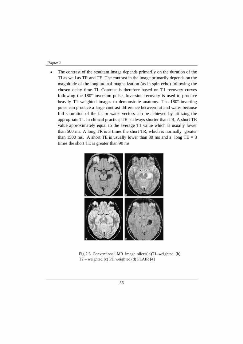
• The contrast of the resultant image depends primarily on the duration of the TI as well as TR and TE. The contrast in the image primarily depends on the magnitude of the longitudinal magnetization (as in spin echo) following the chosen delay time TI. Contrast is therefore based on T1 recovery curves following the 180º inversion pulse. Inversion recovery is used to produce heavily T1 weighted images to demonstrate anatomy. The 180º inverting pulse can produce a large contrast difference between fat and water because full saturation of the fat or water vectors can be achieved by utilizing the appropriate TI. In clinical practice, TE is always shorter than TR, A short TR value approximately equal to the average T1 value which is usually lower than 500 ms. A long TR is 3 times the short TR, which is normally greater than 1500 ms. A short TE is usually lower than 30 ms and a long TE = 3 times the short TE is greater than 90 ms

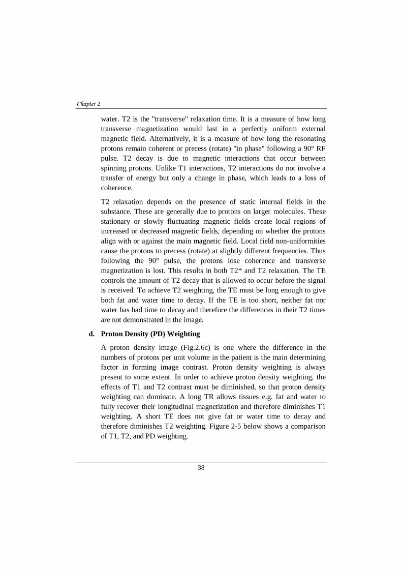
Fig.2.6 Conventional MR image slices(.a)T1–weighted (b) T2 – weighted (c) PD weighted (d) FLAIR [4]


37

a. Soft Tissue Contrast in MRI

Contrast is the means by which it is possible to distinguish among soft tissue types, based on the differences observed in the MRI signal intensities. For example, in musculoskeletal imaging, there is difference in intensities among cartilage, bone, and synovial fluid. In neuroimaging, there are differences between white and grey matter. The fundamental parameters that affect tissue contrast are the T1 and T2 values, proton density, tissue susceptibility and dynamics. Tissue pathology will also affect contrast, as will the static field strength, the type of sequences used, contrast media and the sequence parameters (TR, TE, TI, FA, SNR etc…)

b. T1 Weighting

To demonstrate T1, proton density and T2 contrast, specific values of TR and TE are selected for a given pulse sequence. The selection of appropriate TR and TE weights an image so that one contrast mechanism predominates over the other two. A T1 weighted image(Fig.2.6a) is one where the contrast depends predominantly on the differences in the T1 times between tissues e.g. fat and water. T1 is the longitudinal relaxation time. It indicates the time required for a substance to become magnetized after first being placed in a magnetic field or, alternatively, the time required for regaining longitudinal magnetization following an RF pulse. T1 is determined by thermal interactions between the resonating protons and other protons and other magnetic nuclei in the magnetic environment or "lattice". These interactions allow the energy absorbed by the protons during resonance to be dispersed to other nuclei in the lattice.

All molecules have natural motions due to vibration, rotation, and translation. Smaller molecules like water generally move more rapidly, thus they have higher natural frequencies. Larger molecules like proteins move more slowly. When water is held in hydration layers around a protein by hydrophilic side groups, its rapid motion slows considerably.

c. T2 -Weighting

T2 weighted image (Fig.2.6b) is one where the contrast predominantly depends on the differences in the T2 times between tissues e.g. fat and

Chapter 2

38

water. T2 is the "transverse" relaxation time. It is a measure of how long transverse magnetization would last in a perfectly uniform external magnetic field. Alternatively, it is a measure of how long the resonating protons remain coherent or precess (rotate) "in phase" following a 90° RF pulse. T2 decay is due to magnetic interactions that occur between spinning protons. Unlike T1 interactions, T2 interactions do not involve a transfer of energy but only a change in phase, which leads to a loss of coherence.

T2 relaxation depends on the presence of static internal fields in the substance. These are generally due to protons on larger molecules. These stationary or slowly fluctuating magnetic fields create local regions of increased or decreased magnetic fields, depending on whether the protons align with or against the main magnetic field. Local field non-uniformities cause the protons to precess (rotate) at slightly different frequencies. Thus following the 90° pulse, the protons lose coherence and transverse magnetization is lost. This results in both T2* and T2 relaxation. The TE controls the amount of T2 decay that is allowed to occur before the signal is received. To achieve T2 weighting, the TE must be long enough to give both fat and water time to decay. If the TE is too short, neither fat nor water has had time to decay and therefore the differences in their T2 times are not demonstrated in the image.

d. Proton Density (PD) Weighting

A proton density image (Fig.2.6c) is one where the difference in the numbers of protons per unit volume in the patient is the main determining factor in forming image contrast. Proton density weighting is always present to some extent. In order to achieve proton density weighting, the effects of T1 and T2 contrast must be diminished, so that proton density weighting can dominate. A long TR allows tissues e.g. fat and water to fully recover their longitudinal magnetization and therefore diminishes T1 weighting. A short TE does not give fat or water time to decay and therefore diminishes T2 weighting. Figure 2-5 below shows a comparison of T1, T2, and PD weighting.


39

e. FLAIR (Fluid Attenuate Invesion Recovery)

It is another variation of the inversion recovery sequence. In FLAIR (Fig.2.6d), the signal from fluid (e.g. cerebrospinal fluid (CSF)) is nulled by selecting a TI corresponding to the time of recovery of CSF from 180º inversion to the transverse plane.The signal from CSF is nullified and FLAIR is used to suppress the high CSF signal in T2 and proton density weighted images so that pathology adjacent to the CSF is seen more clearly. A TI of approximately 2000 ms achieves CSF suppression at 3.0T.

f. Contrast agents (Gadolinium)

Although MRI is a very powerful imaging technique not all pathologies are clearly contrasted using only proton density or relaxation times weighting. For example, some meningiomas and small metastatic lesions do not show on normal imaging. And considering that some of these intra-cranial lesions have an abnormal vascular bed or a breakdown of the blood-brain barrier, a magnetic contrast agent that distributes throughout the extracellular space became an obvious choice to improve image contrast.

• All the common contrast agents used in MRI are Gadolinium chelates, which are not directly imaged but produce an effect, which is imaged. Gadolinium is the element of choice because of its high number of seven unpaired electrons. Each unpaired electron has a magnetic moment 657 times bigger than that of a proton, so seven unpaired electrons can induce relaxation a million times better than an isolated proton. This implies that both T1 and T2 are reduced, although the enhancement caused by the shortening of T1 is stronger than the signal loss caused by the shortening of T2; and that is why with Gadolinium contrast the images obtained are normally T1 weighted. The actual amount of T1shortening is dependent on the concentration of Gadolinium injected and the signal enhancement depends also on TE and TR.

2.3.1.2 Applications of MR Imaging in Neoplastic CNS Lesions

Conventional MR imaging is the technique of choice for differential diagnosis, tumor grading, and treatment planning of neoplastic CNS lesions. Alternative imaging modalities (CT, PET) under specific circumstances, are used as a complement to MR imaging. MR imaging represents the technique of choice

Chapter 2

40

for visualizing and grading brain tumors. However, CT, with a lower resolution than MR imaging, does have applications in the emergency situations. The differential diagnosis of tumoral and pseudotumoral (mainly of inflammatory origin) lesions represents a pivotal step in patient assessment that directs subsequent management decisions. Identifying a tumoral lesion at imaging is followed typically by stereotactic biopsy or surgical resection for histologic confirmation. These represent a diagnostic challenge that may require biopsy for definitive diagnosis, which carries significant morbidity and may itself be non-diagnostic [25].

Conventional MR imaging, including T1-weighted, T2- weighted, and contrast-enhanced T1-weighted imaging, frequently provides imaging features that permit an accurate differential diagnosis between tumoral and pseudotumoral lesions in 50% of cases. It provides important information regarding contrast material enhancement, enhancement edema, distant tumor foci, hemorrhage, necrosis, mass effect, and so on, which are all helpful in characterizing tumor aggressiveness and hence tumor grade. It also readily provides evidence of contrast material enhancement, signifying blood-brain barrier breakdown, which is often associated with higher tumor grade. However, contrast material enhancement alone is not always accurate in predicting tumor [26].

Based on the patient's conventional MRI, a radiologist cannot differentiate whether it is a low grade glioma or a high grade glioma, because both of these are almost visually similar [26]. A biopsy is usually required to establish the diagnosis and subtype of a brain tumor and to plan appropriate treatment after conventional MR imaging. The most common conventional MRI modalities used to assess gliomas are Fluid Attenuated Inversion Recovery (FLAIR), T1 and T2-weighted modalities. T1-weighted modalities highlight fat tissues in the brain whereas T2-weighted modalities highlight tissues with higher concentration of water. FLAIR images are T2 or T1-weighted with the cerebrospinal fluid (CSF) signal suppressed. In general, edema, border definition and tumor heterogeneity are best observed on FLAIR and T2-weighted images [34].

Grade detection of glioma tumors is very important for taking clinical decisions regarding the treatment and for finding survival rates without doing biopsy. The major challenges are, tumor characterization is difficult, because the


41

neoplastic tissue is often heterogeneous with conventional MR imaging profile. The second thing is that, the external representation of tumor, which is shape, could not be taken as a discriminant feature for detection/ classification of grade/type of tumor because, the shape of each tumor is not consistent throughout all slices of MR image and may change quickly where the inter-slice distance is large. Advanced MR imaging modalities such as proton MR spectroscopic imaging (MRSI), perfusion-weighted imaging (PWI), and diffusion-weighted imaging (DWI) have been proposed as alternate methods for differential diagnosis of tumors and non tumor lesions, primary versus metastatic lesions and tumor grading [26-28].

2.3.1.3 Clinical Practice of Brain Tumor Imaging

The clinical practice of imaging patients with a suspected brain tumor is a standardized MRI protocol. MRI images are commonly viewed in three planes: axial, coronal, and sagittal as shown Fig. 2.7. Seven different MR sequences are performed to provide a complete MRI data set for one patient. The different sequence properties are shown in Table 2-1.

(a) (b) (c)

Fig.2.7 shows MRI views in three planes a) Axial (b) Sagittal (c) Coronal

Chapter 2

42

Table 2-1: MRI scan protocol for brain tumor patients [35]

Anatomical plane Weighting Contrast Slice thickness / Spacing between

slices

Sagittal ‐ T1‐weighted Nil 5 mm / 6 mm

Axial T1‐weighted Nil 4 mm / 4 mm

Axial T2‐weighted Nil 5 mm / 6 mm

Axial‐ T2‐weighted

FLAIR Nil 5 mm / 6 mm

Axial T1‐weighted Gadolinium 4 mm / 4 mm

Coronal T1‐weighted Gadolinium 4 mm / 4 mm

Sagittal T1‐weighted Gadolinium 5 mm / 6 mm

Twenty slices were acquired for each anatomical plane with TR/TE 2000/45 ms, matrix size 128×128, pixel spacing 1.5×1.5 mm, slice thickness 5.0mm. T1-weighted images are first taken without and then with contrast agent (gadolinium). These images show hyperintense and irregular tumor margins. Surrounding low-signal components correspond to the surrounding brain tissue that is often diffusely infiltrated by tumor cells. Hyperintense tissue that appears in both image types is related to recent bleeding and the tissue that appears hyperintense in T1-weighted contrast enhanced images only, is considered to be malignant tumor [3, 21].

On T2-weighted images the solid part shows hyper intense characteristics [20, 21]. Edema around the tumor shows less hyper-intense signal than the solid tumor part but more intense signal than healthy brain tissue. Both T2-weighted with and without FLAIR can be used to identify edema.

To separate CSF from edema, T2-weighted FLAIR sequences are preferred since the CSF shows no signal. Tumor necrosis is often located in the tumor center. On T2- and T1-weighted images necrosis appears hyper-intense and hyper-iso or hypo-intense, respectively [22-24].


43

Fig. 2.8 shows a glioblastoma in the left temporal lobe acquired in a 1.5 T MRI scanner. A solid mass lesion with edema around the tumor is distinguishable. Fig. 2.8(a) and (b) are T1-weighted and T2-weighted, respectively. A large tumor area consists of necrosis (hypo- and hyper-intense regions on T1- and T2-weighted images, respectively). The edema around the tumor can be identified on the T2-weighted or T2-weighted FLAIR (2.8(c)) images, where it appears hypointense in relation to the bright necrosis. In comparison to the T2-weighted, the CSF on the T2-weighted FLAIR has no hyperintense characteristics. Fig. 2.8d shows the tumor after gadolinium contrast medium application. The tumor borders are well enhanced and the necrosis inside the bright borders is noticeable [23].

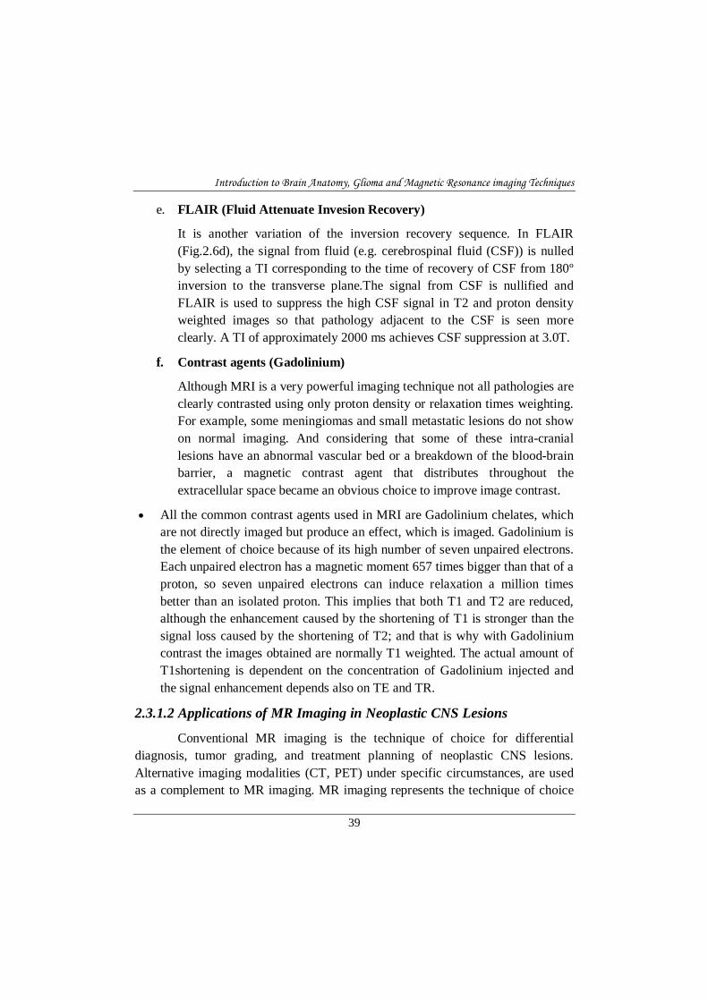
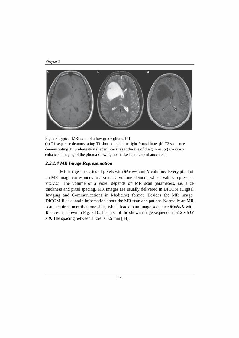
Fig.2.9 shows the MR images of low grade glioma. Fig.2.9 (a) shows T1 pre-contrast image and contrast enhanced low grade glioma is shown in Fig.2.9(c). From the pre and post contrast images, it can be observed that there is no significant intensity variations for tumor necrosis. Usually low grade gliomas are non-enhancing tumors and high grade gliomas are enhancing type. But some low grade more edema will be enhanced by applying contrast agent. Hence this factor alone cannot be taken as a factor for grade detection. Although these images are considered 'typical', numerous studies have questioned the reliability and accuracy of these imaging characteristics for the diagnosis of low-grade glioma.

Fig. 2.8 MR images of a glioblastoma: (a) T1-weighted (b) T2-weighted (c) T2-weighted FLAIR (d) and T1-weighted contrast enhanced [35]

Chapter 2

44

2.3.1.4 MR Image Representation

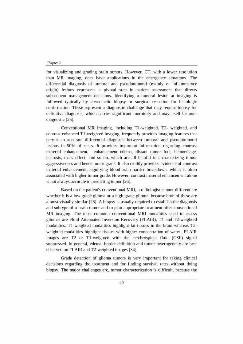
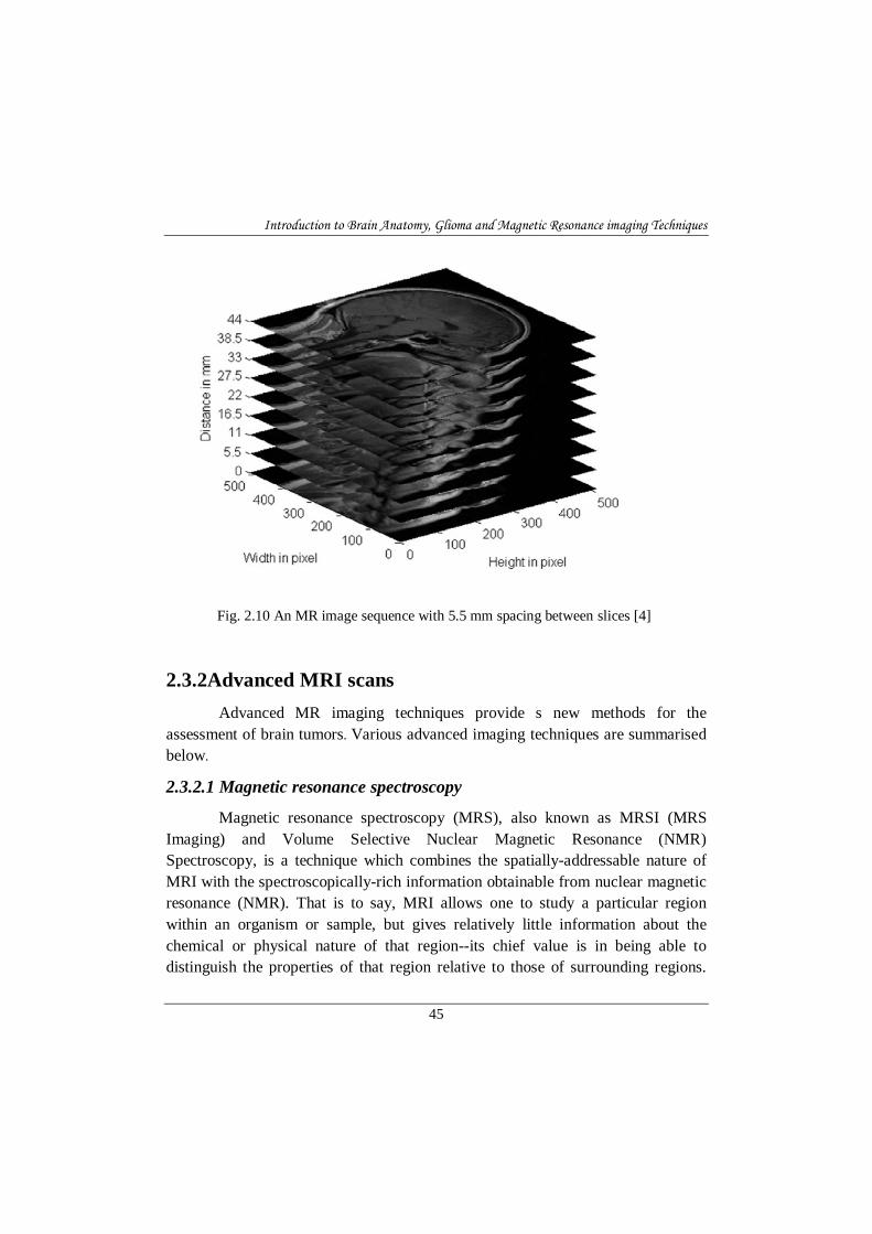
MR images are grids of pixels with M rows and N columns. Every pixel of an MR image corresponds to a voxel, a volume element, whose values represents v(x,y,z). The volume of a voxel depends on MR scan parameters, i.e. slice thickness and pixel spacing. MR images are usually delivered in DICOM (Digital Imaging and Communications in Medicine) format. Besides the MR image, DICOM-files contain information about the MR scan and patient. Normally an MR scan acquires more than one slice, which leads to an image sequence MxNxK with K slices as shown in Fig. 2.10. The size of the shown image sequence is 512 x 512 x 9. The spacing between slices is 5.5 mm [34].

Fig. 2.9 Typical MRI scan of a low-grade glioma [4] (a) T1 sequence demonstrating T1 shortening in the right frontal lobe. (b) T2 sequence demonstrating T2 prolongation (hyper intensity) at the site of the glioma. (c) Contrast-enhanced imaging of the glioma showing no marked contrast enhancement.


45

2.3.2Advanced MRI scans

Advanced MR imaging techniques provide s new methods for the assessment of brain tumors. Various advanced imaging techniques are summarised below. 2.3.2.1 Magnetic resonance spectroscopy

Magnetic resonance spectroscopy (MRS), also known as MRSI (MRS Imaging) and Volume Selective Nuclear Magnetic Resonance (NMR) Spectroscopy, is a technique which combines the spatially-addressable nature of MRI with the spectroscopically-rich information obtainable from nuclear magnetic resonance (NMR). That is to say, MRI allows one to study a particular region within an organism or sample, but gives relatively little information about the chemical or physical nature of that region--its chief value is in being able to distinguish the properties of that region relative to those of surrounding regions.

Fig. 2.10 An MR image sequence with 5.5 mm spacing between slices [4]

Chapter 2

46

MR spectroscopy, however, provides a wealth of chemical information about that region, as would an NMR spectrum of that region [25,26].

2.3.2.2 Functional MRI

Functional MRI (fMRI) measures signal changes in the brain that are due to changing neural activity. The brain is scanned at low resolution but at a rapid rate (typically once every 2-3 seconds). Increase in neural activity cause changes in the MR signal via a mechanism called the BOLD (blood oxygen level-dependent) effect. Increased neural activity causes an increased demand for oxygen, and the vascular system actually overcompensates for this, increasing the amount of oxygenated hemoglobin ("haemoglobin" in British English) relative to deoxygenated hemoglobin. Because deoxygenated hemoglobin reduces MR signal, the vascular response leads to a signal growth that is related to the neural activity. The precise nature of the relationship between neural activity and the BOLD signal is a subject of current research. The BOLD effect also allows for the generation of high resolution 3D maps of the venous vasculature within neural tissue. Likewise, MRI can—within minutes— noninvasively acquire functional images in any plane or volume at comparatively high resolution. Functional MRI (fMRI) can image the hemodynamic and metabolic changes that are associated with human brain functions, such as vision, motor skills, language, memory, and mental processes. These techniques have also revolutionized detection of a wide variety of disease states, such as stroke, multiple sclerosis, and tumors [27].

2.3.2.3 Diffusion MRI

Diffusion MRI measures the diffusion of water molecules in biological tissues. Following an ischemic stroke, brain cells die, trapping water molecules inside them (cellular pumps are no longer functioning). The resultant areas of restricted diffusion are detectable by diffusion weighted imaging (DWI). This finding is identifiable much earlier after a stroke than findings on CT or on conventional MRI, making DWI one of the most sensitive methods for the detection of early stroke [28].

Diffusion MRI (Fig.2.11) is also a tool to study connections in the brain. In an isotropic medium (inside a glass of water for example) water


47

molecules naturally move according to Brownian motion. In biological tissues however the diffusion is very often anisotropic.

For example a molecule inside the axon of a neuron has a low probability to cross a myelin membrane. Therefore the molecule will move principally along the axis of the neural fiber. Conversely, if we know that molecules locally diffuse principally in one direction we can make the assumption that this corresponds to a set of fibers. Diffusion MRI for this application is still at the research stage. Identifying fibers on diffusion MRI is called tractography [29].

DWI is sensitive to motion on the order of tens of micrometers, even locations not commonly noted for motion, such as the brain, move orders of magnitude more than the diffusive motion under investigation, and such motions can corrupt image quality. This effect can mimic increased diffusivity and yield diffusion coefficients that are higher than the true underlying values [30].

2.3.2.4 Diffusion-Tensor Imaging

Diffusion-tensor MR imaging (Fig.2.12) is a technique that has been developed more recently than isotropic (trace-weighted) DW imaging. Typical diffusion-tensor imaging techniques sample water motion in at least six non-

Fig. 2.11 Diffusion weighted Imaging (DWI) slices [23]

Chapter 2

48

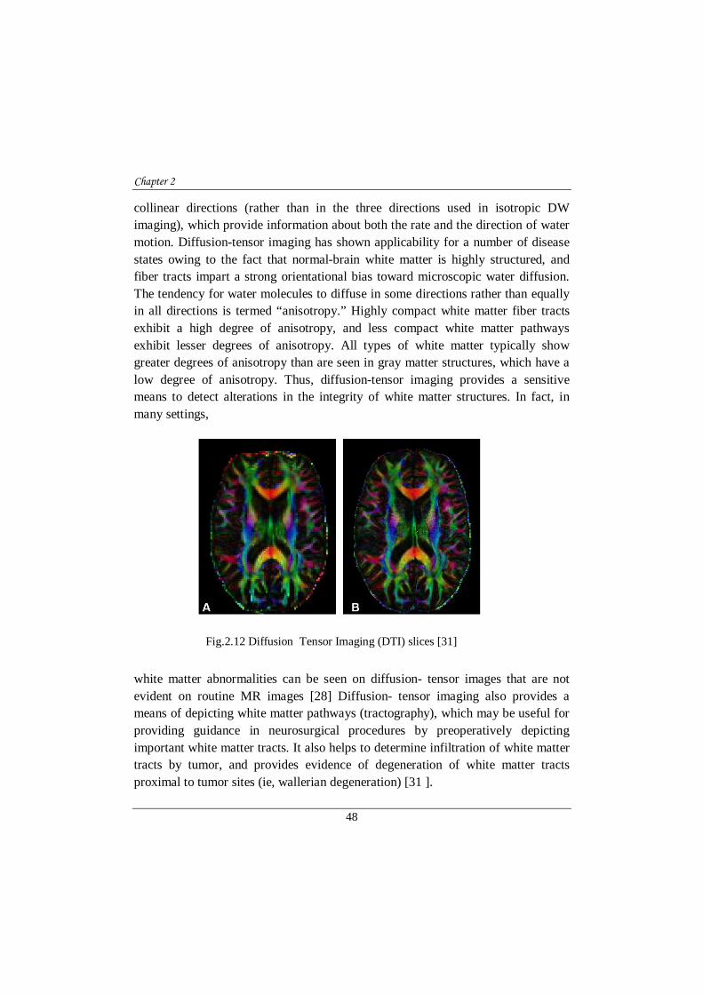
collinear directions (rather than in the three directions used in isotropic DW imaging), which provide information about both the rate and the direction of water motion. Diffusion-tensor imaging has shown applicability for a number of disease states owing to the fact that normal-brain white matter is highly structured, and fiber tracts impart a strong orientational bias toward microscopic water diffusion. The tendency for water molecules to diffuse in some directions rather than equally in all directions is termed “anisotropy.” Highly compact white matter fiber tracts exhibit a high degree of anisotropy, and less compact white matter pathways exhibit lesser degrees of anisotropy. All types of white matter typically show greater degrees of anisotropy than are seen in gray matter structures, which have a low degree of anisotropy. Thus, diffusion-tensor imaging provides a sensitive means to detect alterations in the integrity of white matter structures. In fact, in many settings,

white matter abnormalities can be seen on diffusion- tensor images that are not evident on routine MR images [28] Diffusion- tensor imaging also provides a means of depicting white matter pathways (tractography), which may be useful for providing guidance in neurosurgical procedures by preoperatively depicting important white matter tracts. It also helps to determine infiltration of white matter tracts by tumor, and provides evidence of degeneration of white matter tracts proximal to tumor sites (ie, wallerian degeneration) [31 ].

Fig.2.12 Diffusion Tensor Imaging (DTI) slices [31]


49

2.3.2.5 Perfusion-weighted MRI

Perfusion-weighted MRI (PWI) is an evolving MRI technology for studying cerebral hemodynamics and blood flow (Fig.2.13). Hemodynamic maps of cerebral blood flow (CBF), cerebral blood volume (CBV), and mean transit time (MTT) can be created using PWI. These maps are based on mathematical analysis of the evolution of the intensity of the T2-weighted gradient or spin echo images after a gadolinium bolus administration or by using “labeled” water protons as endogenous, freely diffusible tracers. The advantages of these PWI techniques are their high resolution and non invasive nature compared with PET or CT based methods. PWI can be combined with other MRI techniques such as magnetic resonance angiography (MRA) to assess vessel patency and with DWI to assess ischemic injury. Several problems remain, however, regarding the use of PWI to non invasively quantify CBF and MTT in pathological states. The problems relate to the difficulty of measuring brain density and plasma hematocrit in pathological states and obtaining a value for the relaxivity of gadolinium contrast agent across a range of blood vessel sizes. Other pitfalls include the difficulty of measuring the arterial input function close to the voxel of interest, delay and dispersion of the contrast bolus [32].

Fig.2.13 Perfusion weighted Imaging (PWI) [32]

Chapter 2

50

These advanced MRIs are providing insights into tumor behavior that are not available from conventional MR imaging and will likely be more important for assessment of tumor response to therapy than for diagnosis. DWI may allow the cellularity of tumors to be graded noninvasively; because cells constitute a relative barrier to water diffusion, compared with extra cerebral space, tumors that are more cellular would be expected to show less of an increase in ADC than tumors that are less cellular. Studies of patients with brain tumors have shown that increases in water diffusion generally indicate positive response to therapy.

2.3.3 Noise in MR Imaging Many image acquisition procedures (MRI, PET, SPECT, etc.) suffer from

image degradation by noise. For Magnetic Resonance Imaging the primary source of random noise is thermal noise which forms a statistically independent random source entering the MR data in the time domain. Thermal noise is white and can be characterized by a Gaussian random field with zero mean and constant variance [33]. Hence the noise is not correlated with the signal or with itself. Apart from thermal noise, structured noise usually degrades the image quality as well due to MR system characteristics, physiological pulsations or object motion. The characteristics of noise depend on its source, as does the operator which reduces its effects. Noise, inhomogeneous pixel intensity distribution and blunt boundaries in the medical MR images caused by MR data acquisition process are the main problems that will affect the quality of MRI segmentation [33]. One principal source of noise is the ambient electromagnetic field picked up by the radiofrequency (RF) detectors acquiring the MR signal, and another is the object or body being imaged

In MRIs, raw data is intrinsically complex valued and corrupted with zero mean Gaussian distributed noise with equal variance. After inverse Fourier transformation, the real and imaginary images are still Gaussian distributed, given the orthogonality and linearity of the Fourier transform. MR magnitude images are formed by simply taking the square-root of the sum of the square of the two independent Gaussian random variables (real and imaginary images) pixel by pixel. After this nonlinear transformation, MR magnitude data can be shown to be Rician distributed.


51

In MRI, there is a trade off between signal-to-noise ratio (SNR), acquisition time and spatial resolution. The SNR is relatively high in most MRI applications, and this is accomplished implicitly and explicitly by averaging. The MRI data acquisition process can be affected by two averaging techniques: (1) Spatial volume averaging is required due to the discrete nature of the acquisition process and (2) In the case of some applications, the signal for the same k-space location is acquired several times and averaged in order to reduce noise.

The two averaging methods are interconnected. When a higher sampling rate of the frequency domain is used, higher resolution images are obtained. However, in order to receive a desired SNR at high spatial resolution a longer acquisition time is required, as additional time necessary for averaging. Conversely, the acquisition time, with the subsequent SNR and the imaging resolution, are practically limited by the patient comfort and the system throughput. Consequently, high SNR MRI images can be acquired at the expense of constrained temporal for spatial resolution. Also, high resolution MRI imaging is achievable at a cost of lower SNR for longer acquisition times.

Another important source of noise in MRI imaging is thermal noise in the human body. Common MRI imaging involves sampling in the frequency domain (also called "k-space"), and taking Inverse Discrete Fourier Transform. Signal measurements have components in both real and imaginary channels and each channel is affected by additive white Gaussian noise. Thus, the complex reconstructed signal includes a complex white additive Gaussian noise. Due to phase errors, usually the magnitude of the MRI signal is used for the MRI image reconstruction. The magnitude of the MRI signal is real-valued and is used for the image processing tasks, as well for visual inspection [34,35 ].

The way the magnitude MRI image is reconstructed results in a Rician distribution of noise. Since the Rician noise is signal-dependent, separating the signal from the noise is a very difficult task. In high intensity areas of the magnitude image, Rician distribution can be approximated to a Gaussian distribution, and in low intensity regions it can be estimated as a Rayleigh distribution. A practical effect is, a reduced contrast of the MRI image, as the noise increases the mean intensity values of the pixels in low intensity regions also increases. As explained, it is a fact that Rician noise degrades the MRI images in

Chapter 2

52

both qualitative and quantitative senses, making image processing, interpretation and segmentation more difficult. Consequently, it is important to develop an algorithm to remove this type of noise.

2.3.3.1 Different Noise Models

Noise modeling in images is affected by capturing instrument, data transmission media, image quantization and discrete source of radiation.

a. Gaussian Noise

Gaussian noise is statistical noise that has a probability density function (abbreviated pdf) of the normal distribution (also known as Gaussian distribution). In other words, the values that the noise can take on are Gaussian-distributed. It is most commonly used as additive white noise to yield additive white Gaussian noise (AWGN). Gaussian noise is properly defined as the noise with a Gaussian amplitude distribution. This says nothing of the correlation of the noise in time or of the spectral density of the noise. Labeling Gaussian noise as 'white' describes the correlation of the noise. It is necessary to use the term "white Gaussian noise" to be correct. In Magnetic Resonance Images, raw data is intrinsically complex valued and corrupted with zero mean Gaussian distributed noise with equal variance. After inverse Fourier transformation, the real and imaginary images are still Gaussian distributed given the orthogonality and linearity of the Fourier transform. MR magnitude images are formed by simply taking the square-root of the sum of the square of the two independent Gaussian random variables pixel by pixel.

MR images are corrupted by Rician noise, which arises from complex Gaussian noise in the original frequency domain measurements [36]. The Rician probability density function for the corrupted image intensity x is given by Eqn.4.19

(4.19)

where A is the underlying true intensity, σ is the standard deviation of the noise, and I0 is the modified zeroth order Bessel function of the first kind.


53

b.Speckle noise

A different type of noise in the coherent imaging of objects is called speckle noise. This noise is, in fact, caused by errors in data transmission [36]. This kind of noise affects the ultrasound images [33]. Speckle noise follows a gamma distribution and is given as Eqn.4.20

!

(4.20)

where, a2 is the variance, is the shape parameter of gamma distribution and g is the gray level. Speckle noise is a granular noise that inherently exists in and usually degrades the quality of the active radar and synthetic aperture radar (SAR) images and can also be present in MR images..

2.3.4 Partial volume effect The partial volume effect (PVE) is the consequence of the limited

resolution of the scanning hardware and the discretization procedures. It occurs in non-homogeneous areas, where several anatomic entities contribute to the gray level intensity of a single pixel/voxel. It results in blurred intensities across edges, making difficult the task of accurately deciding on the borders of two connected objects. An example of this type of artifact is the fat/water cancelling and emerging in regions containing both fat and water. Due to their opposing magnetization fields, the corresponding regions will appear dark [34].

Segmentations that allow regions or classes to overlap are called soft segmentations. Soft segmentations are important in medical imaging because of partial volume effects, where multiple tissues contribute to a single pixel or voxel resulting in a blurring of intensity across boundaries. Fig.2.14 illustrates how the sampling process can result in partial volume effects, leading to ambiguities in structural definitions. In Fig.2.14, it is difficult to precisely determine the boundaries of the two objects.

Chapter 2

54

A hard segmentation forces a decision of whether a pixel is inside or outside the object. Soft segmentations on the other hand, retain more information from the original image by allowing uncertainty in the location of object boundaries. Note that the point spread function of an imaging device can be larger than the spatial extent of a single pixel or voxel. Thus, partial volume effects can cause boundaries to be blurred across significant portions of an image.

2.3.5 Intensity in-homogeneities Another difficulty which has to be handled by segmentation techniques

using MR images is the intensity in-homogeneities shortcoming. The intensity in-homogeneities can be caused by the imperfections in the RF coil that produces the magnetic field, or by various defects in the signal acquisition procedures. Also, the magnetic field can have a non-uniform distribution due to the local magnetic properties of the biological structure or because of a movement of the patient during the acquisition process. This effect can be identified as a shading artifact in the image data and can have a major consequence on the performances of the intensity based segmentation algorithms, considering that a certain tissue has a constant intensity distribution in the dataset [35].

Fig. 2.14 A common example of Partial volume effect [7]


55

Conclusions The materials included in this chapter give primary information for the

subsequent discussions of brain anatomy, Glioma, grades, MRI sequences giving basic idea about brain anatomy, tumor and the imaging techniques. This chapter also provides a basic idea about the extent to which the conventional MR imaging techniques are useful for grade detection and visualization of glioma tumors. The different imaging modalities and the different factors which affect the quality of MR image are also presented.

References [1] www.abta.org -- American Brain Tumor Association

[2] www.cbtf.org -- Children's Brain Tumor Foundation

[3] www.virtualtrials.com -- Musella Foundation for Brain Tumor Research and Information

[4] www.braintumor.org -- National Brain Tumor Society

[5] www.neurosurgery.org -- American Association of Neurologic Surgeons

[6] www.cancer.org -- American Cancer Society

[7] www.cancer.gov -- National Cancer Institute

[8] www.asco.org -- American Society for Clinical Oncology

[9] www.cancer.gov/clinicaltrials -- Find clinical trials

[10] www.cancer.net -- Cancer.Net

[11] A. Michotte, Adamson C, Kanu OO, Mehta AI, Di C, Lin N, Mattox AK, et al. Glioblastoma multiforme: a review of where we have been and where we are doing. Expert Opin Investig Drugs, vol.18(8):pp.1061-83.(2009).

[12] D.C Bowers, Y Liu, W Leisenring, et al. Late-occurring stroke among long-term survivors of childhood leukemia and brain tumors: a report from the Childhood Cancer Survivor Study. J Clin Oncol, vol.24(33):pp.5277-82.(2006).

Chapter 2

56

[13] J.C Buckner, P D Brown, O'Neill BP, Meyer FB, Wetmore CJ, Uhm JH. Central nervous system tumors. Mayo Clin Proc, vol.82(10):pp.1271-86.(2007).

[14] Chandana SR, Movva S, M Arora, et.al, Primary brain tumors in adults. Am Fam Physician, vol. 77(10):pp.1423-30.( 2008).

[15] O O. Kanu, A Mehta, C Di, et al. Glioblastoma multiforme: a review of therapeutic targets. Expert Opin Ther Targets, vol.13(6):pp.701-18.(2009).

[16] D Krex, B Klink, C Hartmann, et al. Long-term survival with glioblastoma multiforme. Brain, vol.130(10):pp.2596-2606. (2007).

[17] D A Mitchell, J H Sampson. Toward effective immunotherapy for the treatment of malignant brain tumors. Neurotherapeutics, vol. 6(3):pp.527-538.(2009).

[18] P.C Nathan, S.K Patel, K Dilley, et al. Guidelines for identification of, advocacy for, and intervention in neurocognitive problems in survivors of childhood cancer: a report from the Children's Oncology Group. Arch Pediatr Adolesc Med, vol.161(8):pp.798-806,( 2007).

[19] National Comprehensive Cancer Network. NCCN Clinical Practice Guidelines in Oncology: Central nervous system cancers. Vol.(2).(2009).

[20] S Sathornsumetee, D A Reardon, A Desjardins, et.al. Molecularly Targeted Therapy for malignant glioma. Cancer, vol.110(1):pp.13-24.(2007).

[21] R Stupp, F Roila; ESMO Guidelines Working Group. Malignant glioma: ESMO clinical recommendations for diagnosis, treatment and follow-up. Ann Oncol, vol.20(4):pp.126-128.(2009)

[22] Wen PY, Kesari S. Malignant Gliomas in adults. N Engl J Med, vol.359(5):pp.492-507, (2008).

[23] www.radiologyinfo.org -- RadiologyInfo

[24] M. Essig, N. Anzalone , S.E. Combs, et.al. ‘MR Imaging of Neoplastic Central Nervous System Lesions: Review and Recommendations for Current Practice. AJNR Am J Neuroradiol,vol 33:pp. 803–17 May 2012


57

[25] W. Bian, I. S. Khayal, J. M. Lupo, et.al, Multiparametric Characterization of Grade 2 Glioma using magnetic Resonance Spectroscopic, perfusion, and Diffusion Imaging, Translational Oncology. Vol.2(4) pp.271-280, (2009)

[26] N. Bulakbasi, M. Kocaoglu, A. Farzaliyev et al. Assessment of Diagnostic Accuracy of Perfusion MR Imaging in Primary and Metastatic Solitary Malignant Brain Tumors, Am J Neuroradiol. Vol. 26(9) pp.2187–2199, (2005)

[27] J. M. Provenzale, , S. Mukundan,, P Daniel, et.al Diffusion-weighted and Perfusion MR Imaging for Brain Tumor Characterization and Assessment of Treatment Response Special Review Radiology, vol. 239(3): pp.632-649, (2006).

[28] Neuroimaging and Dissociative Disorders,Angelica Staniloiu1,2,3, Irina Vitcu3 and Hans J. Markowitsch, Chapter 2 Text book on Advances in Brain Imaging, Edited by Vikas Chaudhary, (2012).

[29] M. Law, S. Yang, H. Wang, et.al Glioma Grading: Sensitivity, Specificity, and Predictive Values of Perfusion MR Imaging and Proton MR Spectroscopic Imaging Compared with Conventional MR Imaging AJNR Am J Neuroradiol, vol.24:pp.1989–1998. (2003).

[30] J. M. Provenzale,S. Mukundan, D. P. Barboriak, Diffusion-weighted and Perfusion MR Imaging for Brain Tumor Characterization and Assessment of Treatment Response, Radiology: Volume 239, Number 3, June 2006.

[32] S.cha, Update on Brain Tumor Imaging: From Anatomy to physiology, Am J Neuroradiol, vol. 27 pp.475-87, (2006)

[33] J. Sijbers, P. Scheunders,N. Bonnet,D. Van Dyck, E. Raman. Magnetic Resonance Imaging, Vol. 14, Nr. 10, p. 1157-1163, (1996).

[34] M. V. Sarode, P. R. Deshmukh, Performance Evaluation of Rician Noise Reduction Algorithm in Magnetic Resonance Images, Journal of Emerging Trends in Computing and Information Sciences Volume 2 Special Issue ISSN 2079-8407 2010-11

Chapter 2

58

[35] F. Balsiger, Brain Tumor Volume Calculation Segmentation and Visualization Using MR Images, Department of Biomedical Engineering, Bachelor Thesis, University of Applied Sciences and Arts of Northwestern Switzerland, Switzerland, July 2012.

[36] B. Shinde, D. Mhaske, M. Patare, A.R. Dani. Apply Different Filtering Techniques To Remove The Speckle Noise Using Medical Images. International Journal of Engineering Research and Applications (IJERA) vol. 2( 1): pp.1071-1079.(2012).

chapter 2 introduction to brain anatomy, glioma and magnetic resonance ...shodhganga.inflibnet.ac.in...

Documents