chapter 2- from systems to descriptive models 2.1 introduction 2.2 modeling 2.3 a simple database...

Chapter 2- From Systems to Descriptive Models

2.1 Introduction2.2 Modeling2.3 A Simple Database Server Example2.4 The Database Server Example: Multiple Classes2.5 The Database Server Example: Open and Closed Classes2.6 The Database Server Example: a Mixed Model2.7 The Database Server Example: Types of Resources

Chapter 2- From Systems to Descriptive Models

2.8 The Database Server Example: Blocking 2.9 The Database Server Example: Software

Contention 2.10 Database Example: Simultaneous

Resource Possession 2.11 Database Example: Class Switching 2.12 Database Example: Queuing Disciplines 2.13 QN Models 2.14 Concluding Remarks 2.15 Exercises Bibliography

Introduction(1) Performance and scalability are much easier to

guarantee if they are taken into account at the time of system design.

In this chapter, we start to provide a useful framework that can be used by computer system designers to think about performance at design time.

This framework is based on the observation that computer systems, including software systems, are composed of a collection of resources (e.g., processors, disks, communication links, process threads, critical sections, database locks)

that are shared by various requests (e.g., transactions, Web requests, batch processes)

Introduction(2) Since resources have a finite capacity of

performing work e.g., a CPU can only execute a finite number of

instructions per second, a disk can only transfer a certain number of bytes

per second, and a communications link can only transmit a

certain number of bits per second waiting lines often build up in front of these

resources, in the same way queues form at bank tellers or at

supermarket cashiers.

Introduction(3)

Thus, the framework used in this book is based on queuing models of computer systems.

These models view a computer system as a collection of interconnected queues, or a network of queues.

This chapter describes the qualitative aspect of the framework while the following chapters introduce more quantitative characteristics.

Modeling(1)

A model is an abstraction or generalized overview of a real system.

The level of detail of a model and the specific aspects of the real system that are considered in the model depend on the purpose of the model.

A model should not be made more complex than is necessary to achieve its goals.

The only completely reliable model of a system is itself (or a duplicate copy).

Modeling(2)

However, it is often infeasible, too costly, or impossible to construct such a prototype model.

Future designed systems are not yet available and physically altering existing systems is nontrivial.

At the other extreme, intuitive models (i.e., relying on the "experience" or "gut instinct" of one's local "computer guru"), although quick and inexpensive, suffer from lack of accuracy and bias.

More scientific methods to model building are then required.

Modeling(3)

There are two major types of more scientific models: simulation andanalytic models.

Simulation models are based on computer programs that emulate the different dynamic aspects of a system as well as their static structure.

Alternatively, the customer workload is generated through a probabilistic process, using random number generators.

Simulation models(1)

The flow of customers through the system generates events such as customer arrivals at the waiting line of a server, beginning of service at any given server, end of service,

and the selection of which device to visit next. The events are processed according to their

order of occurrence in time. Counters accumulate statistics that are used at

the end of a simulation to estimate the values of several important performance measures.

Simulation models(2) For instance, the average response time, T, at a

device (i.e., server) can be estimated as

where Ti is the response time experienced by the ith transaction

and nt is the total number of transactions that visited the server during the simulation.

The value of T obtained in a single simulation run must be viewed as a single point in a sample space.

t

n

ii

n

TT

t

1

Analytic models(1)

Analytic models are composed of a set of formulas and/or computational algorithms that provide the values of desired performance measures as a function of the set of input workload parameters.

For analytic models to be mathematically tractable, they are generally less detailed than simulation models.

Therefore, they tend to be less accurate but more efficient to run.

Analytic models(2)

For example, a single-server queue (under certain assumptions to be discussed in later chapters) can expect its average response time, T, to be

where S is the average time spent by a typical request at the server (service time) and is the average arrival rate of customer requests to the server

S

ST

1

Modeling(4)

The primary advantages of analytic and simulation models are, respectively: Analytic models are less expensive to construct

and tend to be computationally more efficient to run than simulation models.

Because of their higher level of abstraction, obtaining the values of the input parameters in analytic models is simpler than in simulation models.

Simulation models can be made as detailed as needed and can be more accurate than analytic models.

Modeling(5)There are some system behaviors that analytic

models cannot (or very poorly) capture, thus necessitating the need for simulation.

In capacity planning, the analyst is generally interested in being able to quickly compare and evaluate different scenarios.

Accuracies at the 10% to 30% level are often acceptable for this purpose.

Because of their efficiency and flexibility, analytic models (exact or approximate) are generally preferable for capacity planning purposes.

This is the approach taken in this book.

A Simple Database Server Example(1)

Consider a database server that has one CPU and one disk.

Database transactions arrive to the database server for execution at a certain rate (e.g., 1.5 transactions per second (tps)).

During its execution, a transaction alternates using the processor and the disk, quite likely more than once.

At any point in time, one transaction might be using the CPU and another using the disk, while yet other transactions are waiting to use the CPU or disk.


Thus, the CPU and the disk can each be characterized as a queue with a waiting line and a device that serves transactions

Figure 2.1 (a) shows a graphical representation used to illustrate a queue with a single resource server.

Transactions arrive and wait if the resource is busy, otherwise they start using the resource immediately.

In some cases, there is a single waiting line for multiple resources (e.g., a multiprocessor, a single line for multiple tellers at the bank).


This type of queue is represented in Fig. 2.1 (b).

Here, a transaction waits in line if all m resources are busy

As soon as a resource becomes available, it starts serving one of the transactions waiting in the queue.

Figure 2.1. (a) Single queue with one resource server (b) Single queue with m resource servers.


The notation just described can be used to represent a simple database server, as illustrated in Fig. 2.2.

This figure depicts a network of queues, or Queuing Network (QN).

Elements such as database transactions, HTTP requests, and batch jobs, that receive service from each queue in the QN are generically called customers.

QNs are used throughout this book as a framework to think about performance at all stages within a system's life cycle.

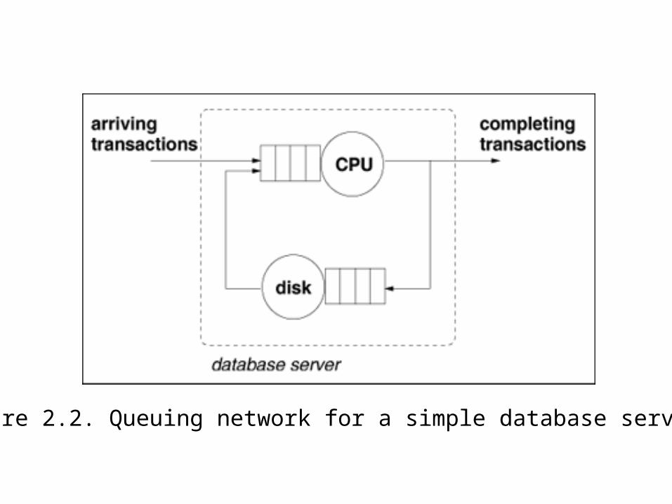
Figure 2.2. Queuing network for a simple database server.


Mapping an existing system into a QN is not trivial. Models are usually built with a specific goal in

mind. For instance, one may want to know how the

response time of database transactions varies with the rate at which transactions are submitted to the database server.

Or, one may want to know the response time if the server is upgraded.

Good models abstract out some of the complexities of real systems while retaining what is essential to meet the model goals.

A Simple Database Server Example(6) For example, the QN model for the database server

example abstracts the complexity of a rotating magnetic disk (e.g., disk controller, disk cache, rotating platter, arm) into a single resource characterized by a single parameter (i.e., the average number of I/Os that the disk can service per second).

However, if one were interested in studying the effect of different disk architectures on performance, then the specific features of interest in the I/O architecture would have to be explicitly considered by the model.

In order to use a QN model of the database server to predict performance for a given transaction arrival rate (e.g., 1.5 tps)

A Simple Database Server Example(7) one needs to know how much time a typical

transaction spends using the CPU and the disk (i.e., the total service time required by a transaction at the CPU and disk).

The model is then used to compute the waiting time of a transaction at the CPU and at the disk.

The total average service time of a transaction at a resource is called its service demand.

This is an important notion that will be revisited many times in this book.

Waiting times depend on service demands and on the system load (i.e., the average number of concurrent transactions in the system).

The Database Server Example: Multiple Classes(1)

Suppose that an investigation of the database management system log reveals that individual transactions submitted to the database server have significantly different characteristics.

However, also suppose that the analyst notes that these transactions can be grouped into three distinct groups of fairly similar transactions, as indicated in Table 2.1:

trivial medium complex

These transaction groups differ in the average CPU time and average number of I/Os per transaction.


Therefore, it would not be appropriate to characterize the transactions submitted to the database server as a single group.

If they were combined into a single group the resulting model may be too approximate and with large errors.

Thus, when describing a QN model, one has to also specify the classes of customers that use the resources of the QN, the workload intensity of each class, and the service demands at each resource per class.

Transaction Group Percentage of Total Average CPU Time (sec) Avg. Number of I/Os

Trivial 45% 0.04 5.5

Medium 25% 0.18 28.9

Complex 30% 1.20 85.0

Table 2.1. Summary Statistics for the Database Server


A multiclass QN model should be used in the following cases:Heterogeneous service demands.

The requests that form the workload can be clustered into groups that exhibit significantly different service demands on the system resources as is the case in Table 2.1.

Different types of workloads. The types of requests in the workload are

different in nature.


For instance, a database server may be used for both: a) short online transactions and b) a batch workload to generate managerial reports.

Different service level objectives. In this case, different classes of requests have

different service level objectives. For example, the transaction groups of Table

2.1 may have 1.2 seconds, 2.5 seconds ,and 8 seconds, as their acceptable limit on the average response time, respectively.

The Database Server Example: Open and Closed Classes(1)

In the examples of the previous sections, the intensity of the workload was specified as the rate at which transactions arrive to the system.

If the overall arrival rate of transactions is 1.5 tps, the arrival rates per class are

0.675 (= 1.5 x 0.45) tps, 0.375 (= 1.5 x 0.25) tps, and 0.45 (= 1.5 x 0.30) tps for trivial, medium,

and complex transactions, respectively, according to Table 2.1.


A customer class that corresponds to a workload specified in this way is called an open class.

An open class has the following characteristics: Workload intensity specified by an arrival

rate. For each open class, the intensity of the workload is represented by the average number of requests arriving per unit time.

This arrival rate is usually independent of the system state (i.e., it does not depend on the number of other customers in the system).


Unbounded number of customers in the system. As the arrival rate of customers increases, the number of customers in the system modeled by the QN tend to grow without bound.

Throughput is an input parameter. In equilibrium, the throughput of an open class is equal to its arrival rate, and is therefore known.

This results from observing that, in equilibrium, the flow into the system (i.e., the arrival rate) must equal the flow out of the system (i.e., the system throughput).


Consider now that at night, the database server of the previous sections is not available for the execution of online transactions.

Instead, it is used to execute batch jobs that produce managerial reports.

A customer class that represents this type of workload is called a closed class.

The characteristics of a closed class are:


Workload intensity specified by the customer population. For each closed class, the workload intensity is

specified by the number of concurrent requests of that class that are in execution (i.e., the customer population for that class).

For example, one may say that five batch jobs are being concurrently executed to produce reports.

It is typically assumed that as soon as one job finishes, another job from the queue is ready to enter and take its place, thus maintaining a (near) constant number of customers in the system.


Bounded and known number of customers in the system. The number of requests in the system is an

input parameter and is therefore known and bounded.

Throughput is an output parameter. The throughput of a closed class is obtained

when solving the QN model and is a function (among other things) of the customer population for that class.


A QN model in which all classes are open is called an open QN model

and a QN model in which all classes are closed is a closed QN model.

Figure 2.3 depicts a QN with a closed workload. and indicates that as soon as one job completes,

another (equivalent) job is started. Thus, the number of jobs in the system remains

constant.

Figure 2.3. Queuing network for a database server with a closed workload.

The Database Server Example: a Mixed Model(1)

Consider again the database server of the previous sections.

Assume now that management has decided that the online transactions of Table 2.1 and the batch management reports should be allowed to execute at the same time at any time of day.

However, before management commits to this decision,

it needs to know if the database server will be able to support both these workloads while meeting the performance objectives for all of them, as specified in Table 2.2.


The performance goal for online transactions are specified in terms of an upper bound on the average response time.

No limit on response time is set for the batch workload.

However, a lower bound on throughput is specified for that class.

Transaction Group Maximum Average Response Time (sec) Minimum Throughput

Trivial 1.2 -

Medium 2.5 -

Complex 8.0 -

Batch Reports - 20 per hour

Table 2.2. Service Level Agreements (SLAs) for the Database Server


Such performance goals are also called Service Level Agreements (SLAs)

since they represent an agreement between service providers and consumers of a service.

SLAs and QoS objectives are related and sometimes used interchangeably.

SLAs are specified for each class and may involve many different performance metrics such as response time, throughput, and availability.


For example, one may have the following sets of SLAs for the services provided by a Web site:

99.99% availability during the 8:00 a.m.-11:00 p.m. interval, and 99.9% availability at other times.

Maximum of four seconds of page download time for all requests submitted over non-secure connections and maximum of six seconds of page download time for requests submitted through secure connections.

Minimum throughput of 2,000 page downloads per second.


The QN model required to answer the performance questions at the beginning of this section is a multiclass mixed QN model.

It is mixed because some classes are open and some are closed.

The representation of this model for the database

server example is shown in Fig. 2.4.

Figure 2.4. Mixed queuing network for a database server.

The Database Server Example: Types of Resources(1)

Suppose that the database server of the previous sections is used to support a client/server application.

Client workstations are connected to the database server through a local area network (LAN).

Clients work independently and alternate between "thinking" (i.e., composing requests to be submitted to the database server) and "waiting" for a reply from the server.

When a reply returns to a client workstation, another thinking/waiting cycle starts immediately.


Therefore, we can represent the time spent at the client (i.e., the think time) as a resource that has no waiting line.

This type of resource is called a delay resource, which we represent by a circle (without the rectangle that represents the queue).

The LAN that connects clients to servers is an Ethernet LAN, whose effective bandwidth decreases as the number of client workstations increases due to increased packet collisions. Thus, the LAN can be modeled as a resource that has a service rate that depends on its load.


This type of resource is called a load-dependent resource

and is represented graphically as a circle with an arrow plus a rectangle to represent the queue.

Resources, such as the CPU and disk, that have a queue but have a constant service rate, are called load-independent resources.

Figure 2.5 depicts the complete QN model with the clients represented as a delay resource, the LAN as a load dependent resource, and database server consisting of two load independent resources.

Figure 2.5. QN for database server with clients and LAN.


To summarize, three types of resources can be used in QN models: Load independent (LI).

These resources have a constant service rate that does not depend on the load (i.e., on the number of requests in the queue).

Load-dependent (LD). The service rate of this type of resource is a

function of the number of requests in the queue.

This type of resource can be used, for example, to model a queue with m resources as in Fig. 2.1 (b).


Delay (D). There is no waiting line in this case. A request that arrives at a delay resource is

served immediately. This type of resource is used to model

dedicated resources (i.e., resources not shared with other requests) or situations in which there is an ample number of resources compared to the number of requests in the system.

The Database Server Example: Blocking(1)

Suppose now that the IT managers of the database service want to provide a response time guarantee to their customers.

In order to provide this guarantee, regardless of the arrival rate of requests, the number of concurrent database transactions has to be limited.

In other words, some form of admission control has to be implemented (see Fig. 1.4).

With an admission control, a limit, W, is set on the number of transactions allowed into the system.


An arriving transaction that finds W transactions in the system is blocked (i.e., it is either rejected or placed in a queue waiting to enter the system).

This is illustrated in Fig. 2.6, which shows the variation of the number of requests in the system versus time.

Each arrow pointing upwards indicates an arrival. At arrival instants, when the load is less than W,

the number in the system increases by one. Downward arrows indicate departures; at these

instants, the number in the system decreases by one.


Downward arrows indicate departures; at these instants, the number in the system decreases by one.

The picture shows five requests arriving when the number of requests in the system is at its maximum value, W. These requests are blocked.

Examples of mechanisms that limit the number of requests in a system include the maximum number of TCP connections handled by a Web server, the

maximum number of database connections supported by a database server, and limits on multiprogramming level enforced by the operating system.

Figure 2.6. Number of transactions in the

database server vs. time with admission control.


Limiting the total number of requests allowed in a computer system limits the amount of time spent by requests at the various queues and therefore guarantees that the response time will not grow unbounded.

This is a type of congestion or admission control. Clearly, if requests are rejected, they will have to

be resubmitted at a latter time.


Figure 2.7 shows the QN for the database server with admission control indicating that transactions are rejected when the system is at its limit.

It should be noted that in this case, the throughput is not necessarily equal to the arrival rate.

In fact: jectionofyprobabilitRateArrivalThroughput Re 1

Figure 2.7. Database server QN with admission control

The Database Server Example: Software Contention(1)

Suppose that the database server is now multithreaded.

Each thread handles one transaction at a time and there is a maximum number of threads.

If all threads are busy serving requests, incoming transactions must queue for an available thread.

An important tuning decision is to determine the the optimal number of threads for a given arrival rate so that the system SLAs are met.

In this situation, there are two opposing effects.


One, called software contention, represents the time that a transaction needs to wait for an available thread.

The other, called physical contention, is the time spent by a transaction waiting to use physical resources (e.g., CPU and disk).

As the number of threads m increases, software contention decreases but physical contention increases because more transactions will be contending for the CPU and disk.


Thus, response time may increase or decrease as a function of m, depending on which factor (software contention or physical contention) dominates, as illustrated in Fig. 2.8.

The picture shows two graphs of response time vs.

number of software threads for two values of the average arrival rate where

The curve for shows the optimal value, m*, for the number of threads that minimizes the average response time for

21 and 21

1

1

Figure 2.8. Response time vs. number of threads for two values of the average arrival rate 21 and


Figure 2.9 illustrates the queue for m software threads.

The figure also indicates the QN that models the physical resources used by the busy threads.

Methods for solving QNs that represent software contention are given in [6, 8]

and are presented in Chap. 15.

Figure 2.9. Database server with software

contention.

Database Example: Simultaneous Resource Possession(1)

Consider now that there is significant update activity in the database server

and therefore, transactions need to acquire a database lock before they can update the database.

Once a lock is acquired, a database transaction will either use the CPU or the disk while holding the database lock.

Thus, two resources will be held by the transaction at the same time (i.e., a database lock and the CPU, or a database lock and the disk).

This situation is called simultaneous resource possession (SRP).


In an SRP situation, a customer in a QN is allowed to hold one or more resources at the same time.

A slightly different, yet equivalent, view is that a customer is executing in parallel, both at the database server lock and at the resource (i.e., CPU or disk) server.

Figure 2.10 shows three time axes: one for the CPU,one for the database lock, and another for the disk.

The picture shows how a transaction spends time waiting and holding each of these resources.

Figure 2.10. Time axes illustration of SRP.


Figure 2.11 illustrates the QN with a queue for database locks.

Dashed arrows from the database locks to the CPU and disk indicate that database locks are held simultaneously with these two resources.

The probability that a lock requested by a transaction is being held by another transaction increases with the system load.

See [9] for analytic models with database locking mechanisms.


Queuing networks with SRP can also be used to model software contention.

In this case, a software resource (e.g., a thread or a critical section) is being held simultaneously with another physical resource (e.g., a CPU or disk).

Similarly, SRP can model other types of hardware contention (e.g., a bus in a shared-memory multiprocessor is held while a memory module is used).

Figure 2.11. QN with simultaneous resource possession. Database locks are held

simultaneously with the CPU and with the disk.

Database Example: Class Switching(1) Consider now a situation in which a user is

required to authenticate itself to the database server before a transaction is executed.

Authentication protocols may use some form of cryptography, which is compute-intensive [7].

Thus, the service demand of a database transaction at the CPU varies significantly depending on whether the transaction is in the authentication phase or in the database access phase.

Figure 2.12 illustrates the various phases of a transaction.

When the service demands in each phase vary widely, one can use a modeling technique called class switching

Database Example: Class Switching(2)

Section 2.4 introduced the notion of multiple classes in a QN model;

different classes can be used to model customers with very different service demands.

In this case, a customer of the QN belongs to a single class.

In class switching, a customer may switch from one class to another when moving between queues.

Figure 2.12. States of a database transaction.

Database Example: Class Switching(3)

In the multiple class case, service demands are associated with a class and a queue.

In addition, however, class switching probabilities, Pi,r;j,s, are used to indicated the probability that a class r customer switches to class s when moving from queue i to queue j.

Class switching is used in [2] to analyze the performance of Kerberos-based authentication protocols.

Database Example: Queuing Disciplines(1)

Suppose that the database server is serving both queries and update transactions

and that the response time SLA of queries is more important than that of update transactions.

In this case, queries should be given preferential treatment, such as a higher priority at the CPU, so that they execute faster than updates.

Many different queuing disciplines can be considered in a QN: First Come First Served (FCFS). Customers are

served in the order of arrival at a queue, as in a supermarket cash register.


Priority Queuing. When the server becomes available, the customer that has the highest priority is served next. If there is more than one customer with the

same priority, FCFS is used to break the tie within each priority class.

There are many possible variations of priority-based queuing disciplines: static priorities vs. dynamic priorities, preemptive vs. non-preemptive, preemptive resume vs. preemptive restart.


In the static priority case, the priority of a customer does not change with time.

With preemptive priority, arriving customers of higher priority are allowed to immediately seize a resource that is being used by a customer of lower priority.

Preempted customers may continue from where they left off (the preemptive resume case) or they may have to to restart (preemptive restart).

Chapter 11 present results for single queues with priorities and

Chapter 15 discusses approximation results for QNs with queues that use priority-based queuing disciplines.


Round Robin (RR). In this case, each transaction is served for a short period of time, called a quantum or timeslice, after which the resource is switched to the next

transaction in a circular fashion. Thus, if there are n transactions in a queue, the

resource allocates a timeslice to transactions in the following order: 1, 2, ···, n, 1, 2, ···.

This type of scheduling discipline is commonly used by operating systems to schedule the CPU to the set of ready processes.


Processor Sharing (PS). This is the theoretical limit of RR as the time slice approaches zero. Another way of thinking about PS when there

are n transactions in a queue is that all n of them are served simultaneously, but each one sees a resources n times slower.

It is typical to assume for modelling purposes that the context switch time for all queuing disciples is negligible.


Many other queuing disciples are possible and have been analyzed, including shortest job first, multi-level feedback, Last Come First Serve-Preemptive Resume

(LCFS-PR), and random.

QN Models(1)

A more formal and complete definition of a QN model is given here.

A QN is a collection of K interconnected queues. A queue includes the waiting line and the

resource that provides service to customers. Customers move from one queue to the other

until they complete their execution and may be grouped into one or more customer classes.

In some cases, customers may be allowed to switch to other classes when they move between queues.

QN Models(2)

A QN can be open, closed, or mixed depending on its customer classes: open if all classes are open, closed if all classes are closed, and mixed if some classes are open and some

are closed. The solution of open, closed, and mixed QNs

under certain assumptions was first presented in [1] and is discussed in more detail in Part II.

QN Models(3)

The input parameters to a QN model are divided into two groups:Workload intensity. These parameters provide

an indication of the load of the system.It can be measured in terms of arrival rates for

open classes or in terms of customer population for closed classes.

QN Models(4)

Service demands. These parameters specify the total average service time provided by a specific resource to a given class of requests. Service demands do not generally depend on

the load on the system. In some situations, however, there may be a

dependence. An example is the service demand on the

paging disk, which is a function of the page fault rate.

In a poorly tuned system, the number of page faults may increase with the number of jobs.

QN Models(5)

Workload classes can also be characterized as transaction, batch, and interactive.

A transaction workload is modeled as an open class with a workload intensity represented by an arrival rate (see the example of Section 2.3).

A batch workload is modeled as a closed class whose workload intensity is represented by the number of customers of that class in the QN (see the example of a report generation class in Section 2.5).

QN Models(6) An interactive workload is a closed class used to

model situations where requests are submitted by a fixed number, M, of terminals or client machines.

The workload intensity in this case is represented by the number of terminals M and by the average think time, Z.

The think time is defined as the time elapsed since a reply to a request is received until the next request is submitted by the same terminal or client (see the client/server example of Section 2.7).

Table 2.3 summarizes the parameters that must be specified for each of these three types of workloads.

Table 2.3. Parameters per Class Type

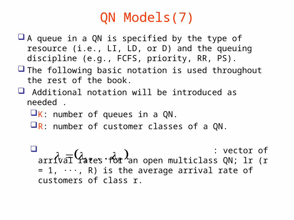
QN Models(7) A queue in a QN is specified by the type of

resource (i.e., LI, LD, or D) and the queuing discipline (e.g., FCFS, priority, RR, PS).

The following basic notation is used throughout the rest of the book.

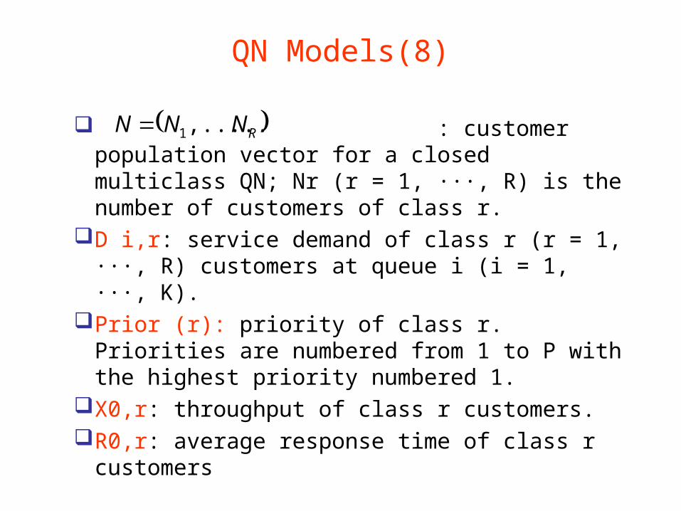
Additional notation will be introduced as needed .K: number of queues in a QN.R: number of customer classes of a QN.

: vector of arrival rates for an open multiclass QN; lr (r = 1, ···, R) is the average arrival rate of customers of class r.

R ,.....,1

QN Models(8)

: customer population vector for a closed multiclass QN; Nr (r = 1, ···, R) is the number of customers of class r.

D i,r: service demand of class r (r = 1, ···, R) customers at queue i (i = 1, ···, K).

Prior (r): priority of class r. Priorities are numbered from 1 to P with the highest priority numbered 1.

X0,r: throughput of class r customers.R0,r: average response time of class r

customers

RNNN ,.....,1

QN Models(9)

QNs may also exhibit characteristics such as blocking, SRP, contention for software resources,and class-switching.

Example 2.1.(1)

Consider the example of Section 2.4 and the data in Table 2.1.

Assume that the total arrival rate is 1.5 tps and that each I/O takes an average of 0.01 seconds.

Thus, the service demand at the disk for each class is equal to the average number of I/Os multiplied by the average time per I/O.

For example, the service demand at the disk for trivial transactions is 0.055 (= 5.5x0.01) seconds.

Example 2.1.(2)

A complete description of the QN for the example of Section 2.4 is given in Table 2.4.

By solving this QN using the methods and tools presented in later chapters of this book, the following response times are obtained: R0,1 = 0.23 sec, R0,2 = 1.10 sec, and R0,3 = 5.08 sec.

(tps)

Table 2.4. QN Specification for Example 2.1

Example 2.2.(1)

Consider now the QN shown in Fig. 2.3. Assume that two batch applications execute

concurrently to generate management reports at night when no online activity is allowed.

One of the applications generates sales reports and the other generates marketing reports.

Both are multithreaded processes. The first application runs as a collection of five

threads and the second as a collection of ten threads.

Example 2.2.(2)

Each thread generates one report A complete description of the QN for the example

of Section 2.4 is given in Table 2.5. By solving this QN using the methods and tools

presented in later chapters of this book, one obtains the following throughputs: X0,1 = 23.2 reports/hour and X0,2 = 24.6 reports/hour.

K = 2; R = xs2

Closed QN

Queue type/Sched. Discipline

LI/PS LI/FCFS

Class (r) Type Nr DCPU,r (sec) Ddisk,r (sec)

1 (Sales) closed 5 45 50

2 (Marketing) closed 10 80 96

Table 2.5. QN Specification for Example 2.2

Concluding Remarks(1)

The exercise of modeling (i.e., abstracting a real system into some kind of representation) has many advantages.

First, several properties of the real system can be elicited in the process of building a model.

For example, sources of contention and the nature of the workload are better understood when a model is built.

Second, a model is a useful guide on what type of measurements to take and what kind of data to collect.


One should restrict the data collection effort to the data necessary to obtain input parameters for the model and to validate the model against the real system.

Third, a number of interesting metrics can be readily computed from the input parameters even before the model is solved.

For example, as it will be shown later in the book, one can obtain bounds on throughput and response time from service demands.


Lastly, a model can be used to answer what-if questions about a real

system, avoiding costly and time-consuming experiments.

The following chapters of this book provide the quantitative aspects necessary to use queuing models for capacity planning and performance prediction.

Most of the models are implemented in MS Excel workbooks, which makes them easy to use.

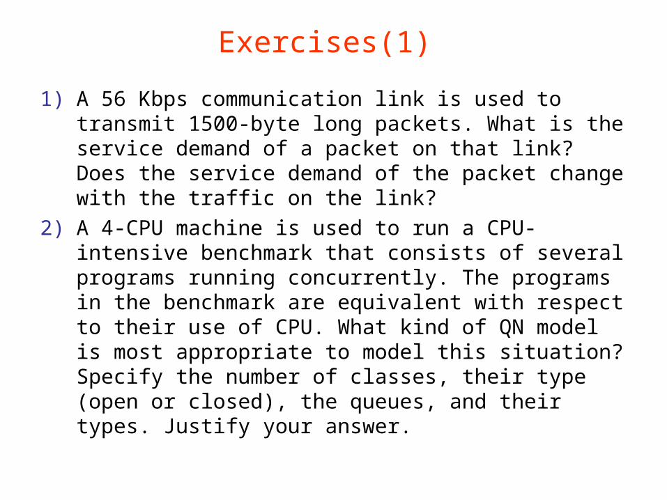
Exercises(1)

1) A 56 Kbps communication link is used to transmit 1500-byte long packets. What is the service demand of a packet on that link? Does the service demand of the packet change with the traffic on the link?

2) A 4-CPU machine is used to run a CPU-intensive benchmark that consists of several programs running concurrently. The programs in the benchmark are equivalent with respect to their use of CPU. What kind of QN model is most appropriate to model this situation? Specify the number of classes, their type (open or closed), the queues, and their types. Justify your answer.

Exercises(2)

3. A computer system supports a transaction workload submitting requests at a rate of 10 tps and a workload of requests submitted by 50 client workstations. What kind of QN should be used to model this situation: open, closed, or mixed?

4. A database server has two identical disks. The service demands of database transactions on these disks are 100 msec and 150 msec, respectively. Show how these service demands would change under the following scenarios:

Exercises(3)

Disk 1 is replaced by a disk that is 40% faster. Enough main memory is installed so that the

hit rate on the database server's cache is 30%.The log option of the database management

system is enabled. A log record is generated on disk 2 for each update transaction. Updates account for 30% of the transactions and recording a log record takes 15 msec.

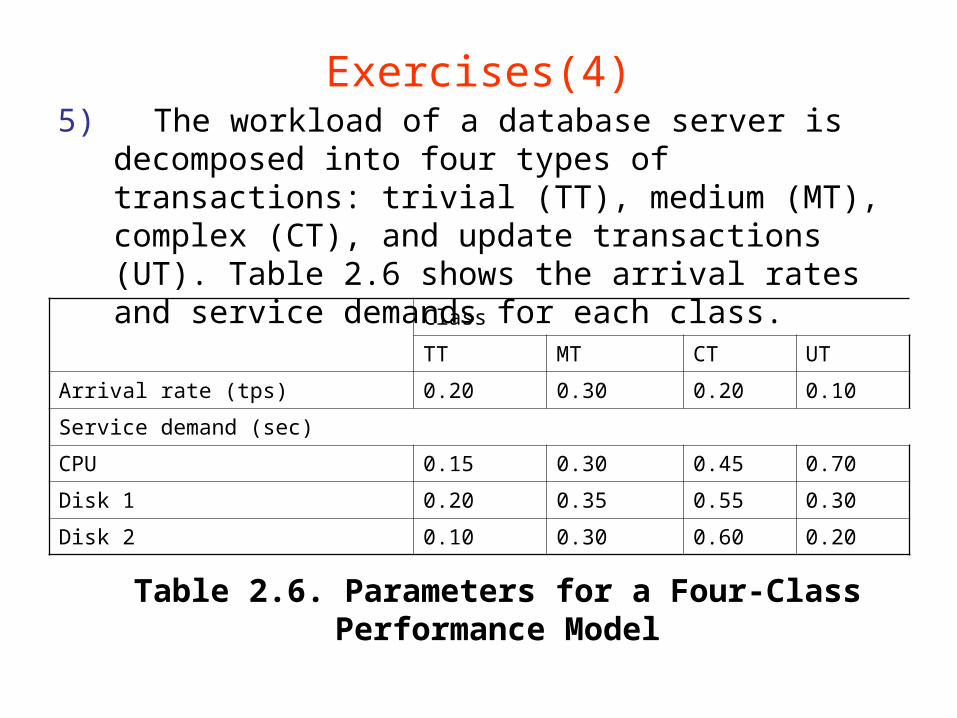
Exercises(4)5) The workload of a database server is decomposed

into four types of transactions: trivial (TT), medium (MT), complex (CT), and update transactions (UT). Table 2.6 shows the arrival rates and service demands for each class.

Class

TT MT CT UT

Arrival rate (tps) 0.20 0.30 0.20 0.10

Service demand (sec)

CPU 0.15 0.30 0.45 0.70

Disk 1 0.20 0.35 0.55 0.30

Disk 2 0.10 0.30 0.60 0.20

Table 2.6. Parameters for a Four-Class Performance Model

Exercises(5) Capacity planners are interested in answering the

following questions: What is the effect on response time of TT

transactions if their arrival rate increases by 50%?

What is the effect on response time of UT transactions if their arrival rate is increased by 25%?

What is the effect on the response time of TT transactions if UT transactions are run on a different machine?

Exercises(6)

From this list of questions, it is clear that the model does not need to consider classes MT and CT separately. How would you aggregate these two classes into a single class? In other words, what is the arrival rate and what are the service demands of the new aggregated class?

6) A delay resource in a QN can be thought as a special case of a load-dependent resource. Give an expression for the service rate m (n) as a function of the number, n, of customers in the resource and of the average service time, S, per customer.

Bibliography(1)

[1] F. Baskett, K. Chandy, R. Muntz, and F. Palacios, "Open, closed, and mixed networks of queues with different classes of customers," J. ACM, vol. 22, no. 2, April 1975.

[2] A. Harbitter and D. A. Menascé, "A methodology for analyzing the performance of authentication protocols," ACM Trans. Information Systems Security, vol. 5, no. 4, November 2002, pp. 458-491.

[3] A. M. Law and W. D. Kelton, Simulation Modeling and Techniques, 3rd ed., McGraw-Hill, New York, 2000.

[4] M. H. MacDougall, Simulating Computer Systems: Techniques and Tools, MIT Press, Cambridge, Mass., 1987.

Bibliography(2)

[5] S. M. Ross, A Course in Simulation, Macmillan, New York, 1990.

[6] D. A. Menascé, "Two-level iterative queuing modeling of software contention," Proc. Tenth IEEE/ACM International Symposium on Modeling, Analysis and Simulation of Computer and Telecommunication Systems (MASCOTS 2002), Fort Worth, Texas, October 12-16, 2002, pp. 267–276.

[7] D. A. Menascé and V. A. F. Almeida, Scaling for E-business: technologies, Models, Performance, and Capacity Planning, Prentice Hall, Upper Saddle River, New Jersey 2000.

Bibliography(3)

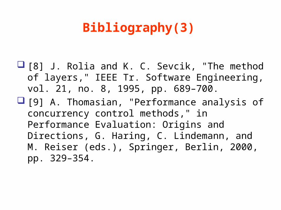
[8] J. Rolia and K. C. Sevcik, "The method of layers," IEEE Tr. Software Engineering, vol. 21, no. 8, 1995, pp. 689–700.

[9] A. Thomasian, "Performance analysis of concurrency control methods," in Performance Evaluation: Origins and Directions, G. Haring, C. Lindemann, and M. Reiser (eds.), Springer, Berlin, 2000, pp. 329–354.

chapter 2- from systems to descriptive models 2.1 introduction 2.2 modeling 2.3 a simple database...

Documents

database example

database locks

computer system designers

real system

software systems

modeling1a model

prototype model

reliable model