chapter 2 experimental set-up and numerical model€¦ · chapter 2 experimental set-up and...
TRANSCRIPT
Chapter 2
Experimental Set-Up and Numerical
Model
In this chapter, the theoretical basis for the investigations carried out within the framework
of the current diploma thesis is given. In addition, the experimental realisation of LACIS
is briefly described.
In the following, the term aerosol will be used repeatedly. An aerosol is defined as a
suspension of liquid and / or solid particles in a gas. In general, the particles are the result
of gas-to-particle conversion (nucleation), the disintegration of liquids or solids, the dis-
persion of powdered material, or the breakup of agglomerates. The diameter size range
of aerosol particles starts at about � nm � ���� m (molecular clusters) and ends at about
����m � ����m (cloud droplets and dust particles). The lower boundary of this range is
determined by the processes leading to new particle formation, in particular nucleation,
i. e. the formation of new particles from gaseous precursors. The upper boundary re-
sults from the important aerosol sink sedimentation. To a certain extent, this boundary
is arbitrary. It has been chosen because particles whose diameter is smaller than ����m
are considered to stay airborne long enough to be observed and measured. Atmospheric
residence times of aerosol particles range from a few hours to several weeks.
5
6 Experimental Set-Up and Numerical Model
2.1 The Experimental Set-Up
Since the present diploma thesis focusses on the numerical analysis of specific aspects,
namely latent heat heat release at the tube wall, equilibrium considerations in the system,
and non-ideality of highly-concentrated solution droplets, only a short overview will be
given on the experimental realisation of LACIS. The device is described in more detail in
Stratmann et al. (2003).
Optical particle measurement
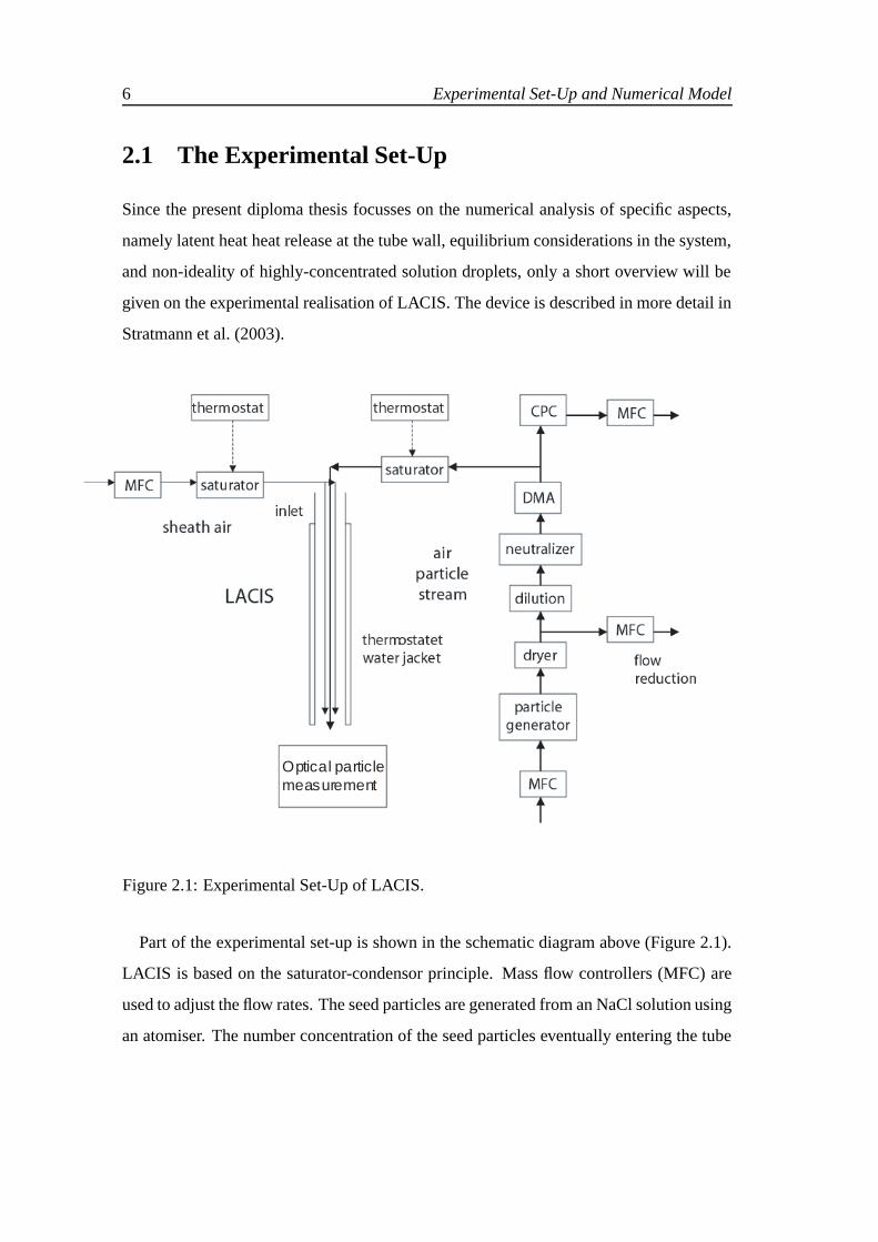
Figure 2.1: Experimental Set-Up of LACIS.
Part of the experimental set-up is shown in the schematic diagram above (Figure 2.1).
LACIS is based on the saturator-condensor principle. Mass flow controllers (MFC) are
used to adjust the flow rates. The seed particles are generated from an NaCl solution using
an atomiser. The number concentration of the seed particles eventually entering the tube
2.1. The Experimental Set-Up 7
as condensation nuclei is adjusted with a dilution system, their size with a Differential
Mobility Analyser (DMA) (Knutson & Whitby, 1975). A Condensation Particle Counter
(CPC) is used to measure the particle number concentration. The relative humidity of
the incoming carrier gas and sheath air is determined by the temperature of the saturator
which can be adjusted by a high-presision thermostat. In the saturator, the previously
dry aerosol is humidified using a Nafion R� tube. LACIS itself then acts as the condenser.
The flow tube is surrounded by a thermostated water jacket whose temperature is kept
lower than the temperature of the mixture entering the tube so that the water vapour starts
to condense. The tube material is quartz glass. Experiments have been carried out for
two different temperatures of the water jacket, ��� ÆC and ���ÆC. The calculations carried
out within the framework of the current diploma thesis have been limited the lower wall
temperature, ��� ÆC. At the tube outlet, an optical sizer is used to measure the size of the
particles.
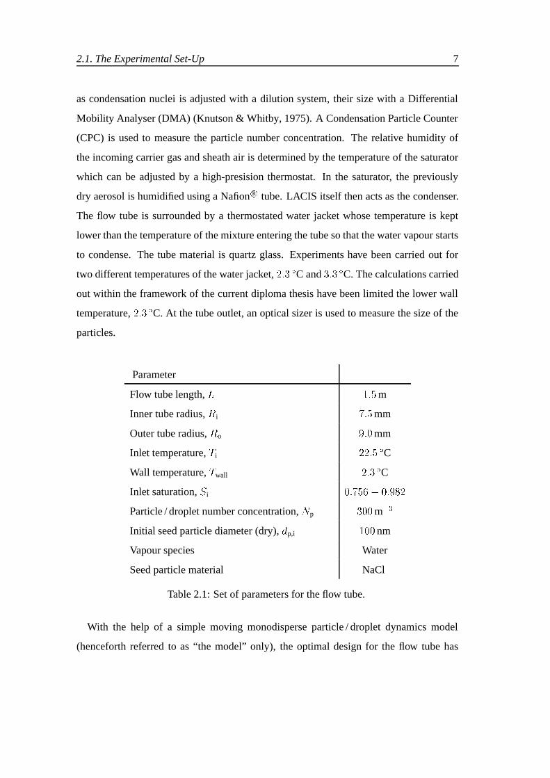
Parameter
Flow tube length, � ���m
Inner tube radius, �i ���mm
Outer tube radius, �o ���mm
Inlet temperature, �i ���� ÆC
Wall temperature, �wall ��� ÆC
Inlet saturation, �i ������ �����
Particle / droplet number concentration, �p ���m��
Initial seed particle diameter (dry), �p,i ��� nm
Vapour species Water
Seed particle material NaCl
Table 2.1: Set of parameters for the flow tube.
With the help of a simple moving monodisperse particle / droplet dynamics model
(henceforth referred to as “the model” only), the optimal design for the flow tube has
8 Experimental Set-Up and Numerical Model
been theoretically determined in order to simulate the atmospheric super-saturations and
time scales associated with the activation and growth of cloud droplets. The model it-
self is described in Section 2.2 (page 9). The geometric and physical parameters decided
upon are given in Table 2.1. The geometric parameters of LACIS are fixed. The physical
parameters are altered to realise a variety of defined thermodynamic states of the aerosol
and sheath air injected at the inlet of LACIS.
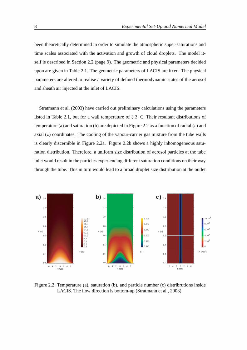
Stratmann et al. (2003) have carried out preliminary calculations using the parameters
listed in Table 2.1, but for a wall temperature of ��� ÆC. Their resultant distributions of
temperature (a) and saturation (b) are depicted in Figure 2.2 as a function of radial (�) and
axial (�) coordinates. The cooling of the vapour-carrier gas mixture from the tube walls
is clearly discernible in Figure 2.2a. Figure 2.2b shows a highly inhomogeneous satu-
ration distribution. Therefore, a uniform size distribution of aerosol particles at the tube
inlet would result in the particles experiencing different saturation conditions on their way
through the tube. This in turn would lead to a broad droplet size distribution at the outlet
6 4 2 0 2 4 6r [mm]
0.0
0.2
0.4
0.6
0.8
1.0
1.2
1.4
3.35.27.19.111.012.914.816.718.720.622.5
T [̊ C]
a)
x [m]
6 4 2 0 2 4 6r [mm]
0.0
0.2
0.4
0.6
0.8
1.0
1.2
1.4
0.940
0.973
1.006
1.040
1.073
1.106
S [ ]-
b)
x [m]
6 4 2 0 2 4 6r [mm]
0.0
0.2
0.4
0.6
0.8
1.0
1.2
1.4
0
2•108
4 108
6 108
8 108
10 108
N [#/m3]
c)
x [m]
Figure 2.2: Temperature (a), saturation (b), and particle number (c) distribrutions insideLACIS. The flow direction is bottom-up (Stratmann et al., 2003).
2.2. The Numerical Model 9
in contrast to the initially-uniform particle size distribution. To avoid such a problem, the
aerosol flux entering the tube is restricted to the tube core; it is surrounded by particle-free
sheath air. The result is an inlet split into two zones. A radius of �mm has been chosen
for the particle beam so that the radial inhomogeneities are minimised. The width of the
particle beam is constant throughout the tube which can be seen in the particle number
concentrations depicted in Figure 2.2c.
LACIS is used in conjunction with the model to improve the understanding of the
activation and growth of particles / droplets that takes place in the early stages of cloud
formation.
2.2 The Numerical Model
The objective of the model is the description of the activation and growth of seed parti-
cles / droplets by vapour deposition. To achieve this objective, the physical processes oc-
curring inside the tube have to be expressed in a mathematical form. The fluid-dynamical
processes like the flow and the coupled mass / heat transfer determine the spatial distribu-
tions of the gas velocity, temperature, and vapour mass fraction. They are linked to the
particle-dynamical processes determining the size distribution and number concentration
of the particles / droplets via the phase transition processes taking place inside the tube.
For example, the water vapour condensing onto the droplets is a sink in the mass transport
equation whereas it is a source in the equation used to calculate the particle / droplet mass
concentration.
Due to rotational symmetry, the tube flow can be regarded as a two-dimensional prob-
lem for the calculations. The flow processes are described by the momentum or Navier-
Stokes equations for two dimensions. For the steady laminar fluid flow realised in LACIS
and accounting for natural convection, the momentum equations for the fluid flow in the
10 Experimental Set-Up and Numerical Model
tube take the form (Bird et al., 1960):
� � ��g � �� � � � ��������
��� �x � �g �x (2.1a)
� � ��g � �� � � � ��������
�� �r � �g �r (2.1b)
where �g is the density of the carrier gas, � � �� �� is the mass average velocity, � is
pressure, �x and �r are viscous terms in addition to those expressed by � � ����� and
�������, � is the dynamic viscosity, � and are the spatial coordinates, and � � ��x �r�
is the gravitational acceleration.
The coupled mass / heat transfer is described by the vapour mass transport and the en-
ergy equation of the vapour-carrier gas mixture. The mass transport is given by (2.2), in
which molecular and thermal diffusion is accounted for:
� � ��g � �v� � �� � �v � �v
�v � ��g v ��v � �g v �v,g ��� �v� �v� ��� (2.2a)
� ��g v ��v � �
v � ��� (2.2b)
Here �v is the vapour mass fraction, �v is the vapour mass flux relative to �, �v is the
vapour sink due to condensation onto the particles / droplets, v is the binary vapour
diffusion coefficient, �v,g is the thermal diffusion factor, and �
v is the thermal (Soret)
diffusion coefficient.
The first term on the right hand side of Equations (2.2a) and(2.2b) represents molecular
diffusion. The vapour diffusion coefficient, v, is a factor of proportionality between
the vapour mass flux, �v, and its concentration gradient, ��v. Diffusion is caused by
the random microscopic motion of gas molecules. This motion is named after Robert
Brown (1773-1858), the botanist who first observed the continuous random movement of
particles in the pollen grains of the American species Clarkia pulchella (common name
Clarkia) in 1827 (Ford, 1992).

2.2. The Numerical Model 11
The second term represents thermal diffusion which is also known as the Soret or
Ludwig-Soret effect. The two expressions given in (2.2) are equivalent. Thermal diffusion
leads to the establishment of a vapour flux when a temperature gradient is maintained in
a binary gas mixture of water vapour and air. For the thermal diffusion coefficient, an
empirically-based composition-dependent expression is used (Fluent, 2001),
��v �� ���� � ���� � � �����
��������
v �v
������v �v �������
g �g� �v
��
�������
v �v �������g �g
������v �v �������
g �g
�(2.3)
It results in a more rapid diffusion of light molecules and a less rapid diffusion of heavy
molecules towards heated surfaces.
The energy equation describes the heat transport due to convection and vapour trans-
port. Accounting for the Dufour effect, which is the opposite to the Ludwig-Soret effect,
the equation takes the following form for a binary mixture, here water vapour in air:
� � ��g � �� � �� � �� �h
� � ��g ��� �g ���v � �v� � v,g mix ��
�v ��g�v (2.4)
where � is the specific enthalpy, � is the heat flux, and �h � �v � �v is the source term for
the latent heat released by the condensation of water vapour onto the particles / droplets
with�v as the latent heat of vapourisation of water. The thermal diffusivity is defined by
� �mix�g �p
, where mix is the heat (or thermal) conductivity of the vapour-carrier gas mix-
ture, and �p is its specific heat capacity at constant pressure. � , �v, and �g respectively
are the molar weights of the vapour-carrier gas mixture, water vapour, and the carrier gas
(air).
The first term on the right hand side of (2.4) represents the influence of conduction heat
transfer in the gas mixture. The second term results from the conversion of temperature
to enthalpy that has been applied to the energy equation to obtain it in the form given in

12 Experimental Set-Up and Numerical Model
(2.4). In the present work, this term is regarded as an additional source term. The third
term represents the Dufour term.
When comparing Equations (2.1), (2.2), and (2.4), certain similarities in their structure
are noticeable. Patankar (1980) states that the dependent variables, which above are �,
�v, and �, obey a generalised conservation principle. Hence, he introduces a general
differential equation, also called general � equation, for the dependent variable �:
�
����g ��
� �� �
Rate of change of �(unsteady term)
�� � ��g ���� �� �
Convectionterm
� � � ������� �� �
Diffusion term
� ������
Source / sinkterm
(2.5)
The diffusion coefficient, ��, and the source term, ��, are specific to the particular
meaning of �. (2.5) is an important equation in numerical modelling since � can stand
for a variety of different quantities.
Sedimenta tion
Diffusion
Nucleation
Evaporation
Condensation
Convection
Other external processes
Coagulation
Figure 2.3: Particle-dynamical transfer and transport processes (Bräsel, 2001). The grey-coloured font indicates processes not considered in the present investigation.

2.2. The Numerical Model 13
Before looking at their numerical realisation, the physical and chemical processes in-
fluencing the particle size and number distribution in a small volume of aerosol are con-
sidered. These processes can be divided into internal and external processes, an overview
is given in Figure 2.3. Internal processes, e. g. nucleation, coagulation, and condensa-
tion / evaporation, take place inside the volume element. Of these processes, only conden-
sation and evaporation have been taken into account in the model. Homogeneous nucle-
ation does not occur at the super-saturations reached inside the flow tube, and coagulation
can be neglected because of the small particle number concentrations (� ���� cm��) in-
vestigated. External processes are characterised by transport across the boundaries of the
volume element, caused e. g. by diffusion, convection, thermophoresis, or sedimentation.
In the model, thermophoresis and sedimentation do not play a significant role (F. Strat-
mann, pers. comm.), so only diffusion and convection are accounted for.
For the transport of particles / droplets due to diffusion and convection as well as their
growth due to condensation, a moving monodisperse model is used. In the present case,
the model solves for the total particle / droplet number concentration, �p, and the par-
ticle / droplet mass concentrations, �p,�, where � denotes the different substances in the
particle / droplet phase:
� � ��g ��p� � � � ��g �p ��p� (2.6)
� � ��g ��p,�� � � � ��g �p ��p,�� ��p��p,�
��(2.7)
Here, �p��p,�
��is the mass of water vapour condensing onto (or evaporating from) the
particles / droplets. This term is therefore identical to v in Equation (2.2), only with the
opposite sign. h � v � v can now be calculated as well.
The convection term, i. e. the left hand side of (2.6), causes a macroscopic particle
motion since the particles are carried along with the flow due to the Stokes drag force.
The term on the right hand side of (2.6) represents particle diffusion caused by the gas
molecules subject to Brownian motion. The particle diffusion coefficient, �p, can be

14 Experimental Set-Up and Numerical Model
calculated using the Stokes-Einstein relation:
�p ��B � �C
� � � �p(2.8)
where �B is Boltzmann’s constant, �p is the particle diameter, and �C is the slip correction
or Cunningham factor. It it necessary to include this factor because the relative velocity
of the gas at the surface of particles whose sizes approach the mean free path � of the gas
(i. e. �p � �m) is not zero. This molecular slip occurs since the particle no longer moves
as a continuum in the fluid, but as a particle among discrete molecules thereby reducing
the drag force and increasing the diffusion coefficient. According to Friedlander (2000),
it can be parametrised as follows:
�C � � ���
�p
����� � �� �
�� ���
�p
�
��(2.9)
The ratio of the mean free path to the particle radius, ���p
, is defined as the Knudsen number.
The particle / droplet growth is described by the second term on the right hand side
of Equation (2.7). The single particle growth law, ��p,�
��, is given by Barrett & Clement
(1988),��p,�
� �
� � �p ��r � �p �v � ����v
�
�v v sat,w �Mass
� ��v p
�v � � �mix �Heat
(2.10)
where is time, �r is the saturation ratio of the vapour phase inside the tube, �p is the
equilibrium saturation ratio at the particle / droplet surface, �v is the specific gas constant
of water vapour, �sat,w is the equilibrium water vapour pressure at temperature � , and �Mass
and �Heat are the mass and heat transfer transition functions.
The saturation ratio �r is defined as the actual water vapour pressure, �, divided by the
ambient equilibrium or saturation water vapour pressure, �sat,w. The temperature depen-
dence of �sat,w is derived in Appendix B.
�p is defined as the ratio of the equilibrium water vapour pressure at the droplet surface,
�sat,dp , to �sat,w. It depends not only temperature, but also on the curvature of the surface
(curvature or Kelvin effect) and on the solute concentration (solution or Raoult effect).
2.2. The Numerical Model 15
The Kelvin effect arises from the fact that the electrostatic forces hindering the molecules
from leaving the curved droplet surface are lower than for a flat liquid surface because
there are fewer attracting neighbouring molecules within any chosen range. It leads to an
increase in the saturation ratio above the droplet. The Raoult effect leads to a decrease
in �p. This decrease can be explained qualitatively since water molecules at the droplet
surface are replaced by solute molecules so that fewer water molecules are able to break
free from the liquid; the equilibrium vapour pressure is reduced.
For a droplet of diameter �p and of solute mole fraction �s, �p is given by
�p � ���
�����
��w �sol
�� �w �p� �� �Kelvin term
�
� s � �s
�w� �� �Raoult term
���� (2.11)
where �sol is the surface tension of the solution droplet, �w � �v is the molar mass of
water, � is the universal gas constant, �w is the density of water, � is the total number of
ions the salt molecule dissociates into, s is the osmotic coefficient of the solute, � is
the volume fraction of the soluble part of the condensation nucleus, and �w is the mole
fraction of water in the droplet. The derivation of (2.11) can be found in Appendix C. The
equation represents one form of the so-called Köhler equations, named after the Swedish
meteorologist H. Köhler. In this form, it can also be found in the model (see the source
code listed in Appendix E).
The Raoult term can be converted to show its dependence on the droplet diameter for a
solution droplet with solute mass �s since
�s
�w�
�s
�� �s
�������
�s �w
�s �w�
�s �w
�s
�sol
�
���p ��s
�
Here, � is mole fraction, � is mass fraction, � is mass, � is molar mass, � is density,
and the indices “s”, “w”, and “sol” refer to “solute”, “water”, and “solution”, respectively.
The density of the solution is determined as the mass weighted average of the densities of

16 Experimental Set-Up and Numerical Model
the compononents, �sol �
��s
�s�
�w
�w
���
. Then,
�p � ���
���w �sol
�� �w �p�
� �s � s �w��s
�sol����p �s
�(2.12)
Plots of �p versus �p, or versus the droplet radius �, are called Köhler curves (Figure
2.4). A growing droplet follows the left branch of the curve for increasing saturation
Figure 2.4: Köhler curves for an aqueous solution droplet of radius � and containing var-ious amounts of NaCl at different temperatures (Bakan et al., 1988).
2.2. The Numerical Model 17
ratio. Once the critical saturation at the critical droplet diameter, i. e. the maximum of
the curve, is reached, the droplet will continue to grow as long as the saturation in the
system is higher or equal to its equilibrium saturation. These droplets are then called
activated droplets.
In the calculations presented in this diploma thesis, the material of the condensation
nucleus is sodium chloride (NaCl) which dissolves into two ions, Na� and Cl�, so that
� � �. For an ideal solution of salt and water in the droplet, �s � � and �� � �, i. e. the
salt dissolves completely. The droplet is assumed to be an ideal solution, although devia-
tions from ideality occur near the tube inlet when the solution of condensation nucleus and
water is highly concentrated. The effects of this non-ideality are investigated in Chapter 5.
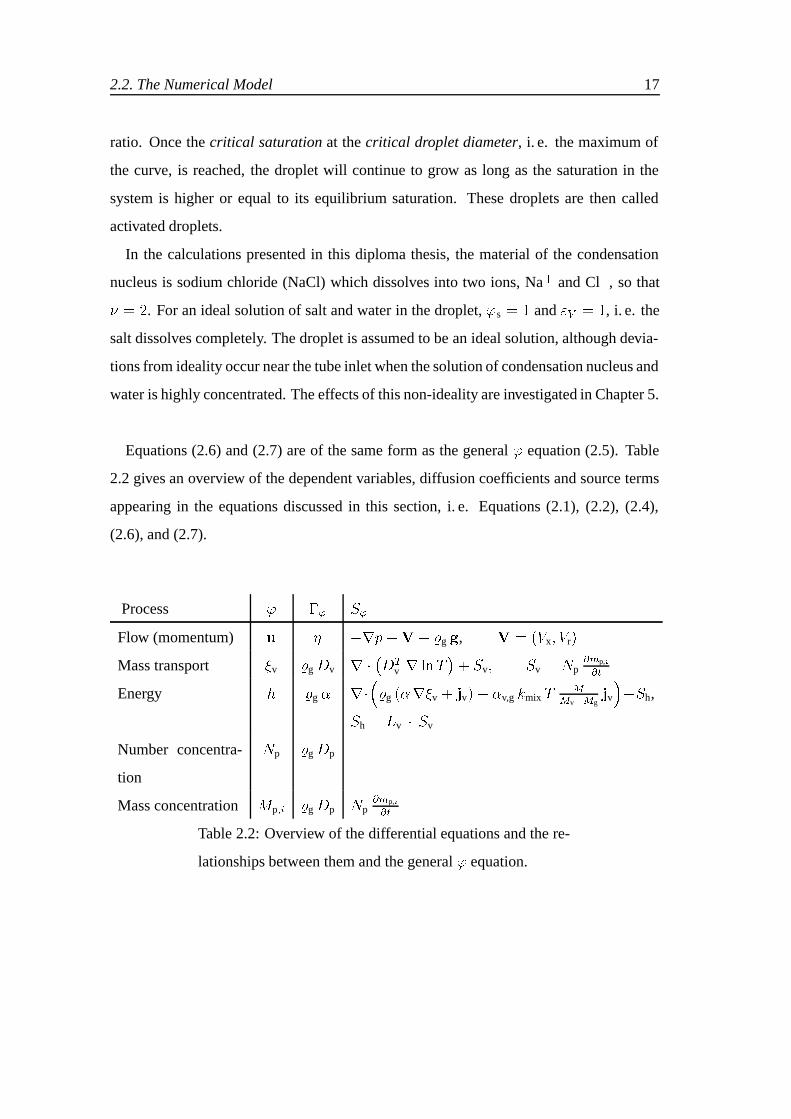
Equations (2.6) and (2.7) are of the same form as the general � equation (2.5). Table
2.2 gives an overview of the dependent variables, diffusion coefficients and source terms
appearing in the equations discussed in this section, i. e. Equations (2.1), (2.2), (2.4),
(2.6), and (2.7).
Process � �� ��
Flow (momentum) � � ��� �� � �g �, � � ��x� �r�
Mass transport v �g v � ���
v � ����� �v� �v � �p
��p,�
��
Energy �g � ��
��g ���v � �v� � �v,g �mix �
��v��g
�v
���h,
�h � �v � �v
Number concentra-
tion
�p �g p
Mass concentration �p�� �g p �p��p,�
��
Table 2.2: Overview of the differential equations and the re-
lationships between them and the general � equation.

18 Experimental Set-Up and Numerical Model
2.3 Realisation of the Numerical Model
Before giving a detailed explanation of the moving monodisperse model used for the
present diploma thesis, the grid will be briefly commented on. It has been created with
GAMBIT, a preprocessor to FLUENT (Fluent, 2001). The calculation domain is split into
separate control volumes, whose density depends on the expected gradients. Hence, the
grid for the presented problem is densely meshed at the inlet, at the tube wall, and at the
boundary between aerosol and sheath air. These densely-meshed areas are clearly recog-
nisable in Figure 2.5.
In FLUENT, the governing differential equations, which include Equations (2.1), (2.2),
(2.4), (2.6), and (2.7), are discretised for the individual control volumes, and then lin-
earised to obtain the values of the dependent variables. These values are used as updates to
solve the discretised equations iteratively until convergence is reached. A short overview
of the numerical scheme used for the calculations can be found in Appendix A.
The mixture of water vapour and carrier gas (air) is realised by enabling the “species
transport”, an option available in FLUENT to characterise the system. The properties of
the mixture are defined by introducing the new material “mixture” which can be thought
of as a set of species and a list of rules governing their interaction. The composition of
the mixture is defined at the tube inlet where the species mass fractions are specified.
The fluid-dynamical processes, i. e. the flow and the coupled mass / heat transfer, are
part of FLUENT’s standard packages. The particle number concentration and the mass
concentrations of the solute and of the liquid water, which are defined respectively as
kilogram of solute or liquid water per kilogram of the vapour-carrier gas mixture, have
to be introduced as so-called User-Defined Scalars (UDS). For such scalars, FLUENT
solves a transport equation of the form of the general � equation. The diffusion coeffi-
cients and source / sink terms of the scalars are determined with the help of a User-Defined

2.3. Realisation of the Numerical Model 19
r [mm]09 7.5
x [m]
1.5
Figure 2.5: Computational grid used in the calculations presented in this diploma thesis.The tube inlet is at the bottom, the outlet at the top. The boundary between thetube interior and the tube wall is indicated by the dark grey line at � � ���mm.In the �-direction, a part of the grid has been removed.
20 Experimental Set-Up and Numerical Model
Function (UDF), which is written in the C programming language. It consists of several
sub-functions, or macros, whose form is pre-defined by FLUENT. In the present case,
a “DEFINE_ADJUST” function is called by FLUENT at the beginning of each iteration
prior to the solution of the govering differential equations. With this function, the par-
ticle / droplet growth inside the tube is determined based on the previous iteration. The
droplet growth influences the energy equation (2.4) due to the release of latent heat of the
water vapour condensing onto the droplets, as well as the transport equations for water
vapour (2.2) and liquid water (2.7) since a phase transition between the vapour and the
liquid phase occurs. These source / sink terms are programmed as “DEFINE_SOURCE”
functions. FLUENT then accesses these functions and includes them in the appropriate
differential equations.
User-specific diffusion coefficients, for the current model the binary vapour diffu-
sion coefficient, �v, and the particle dffusion coefficient, �p, are made available by the
“DEFINE_DIFFUSIVITY” macro. Other macros used in the model are “DEFINE_PROP-
ERTY”, and “DEFINE_PROFILE”. “DEFINE_PROPERTY” allows the use of parametri-
sations other than the ones given internally by FLUENT for material properties. Using
this macro, the heat conductivity of the mixture, �mix, is calculated. With the help of a
“DEFINE_PROFILE” macro, the vapour mass fraction at the tube wall is derived assum-
ing a saturation ratio of �.
The UDF provides the means to solve Equations (2.1), (2.2), (2.4), (2.6), and (2.7). The
equations are solved simultaneously by FLUENT to determine the velocity, temperature,
vapour mass fraction, and saturation fields as well as the particle concentrations (number
and mass) inside the flow tube. The particle / droplet diameter is determined from the
droplet mass concentration. The moving monodisperse model introduced in this section
and realised as a UDF in FLUENT can therefore be used to describe the activation and
growth of particles / droplets by vapour deposition.
In Appendix D, the parametrisations used in the model are given. The source code of
the model is listed in Appendix E.