chapter 2 · oecd economic outlook,volume 2016 issue 2 © oecd 2016 63 chapter 2 using the fiscal...
TRANSCRIPT

OECD Economic Outlook, Volume 2016 Issue 2
© OECD 2016
63
Chapter 2
USING THE FISCAL LEVERSTO ESCAPE THE LOW-GROWTH TRAP
2. USING THE FISCAL LEVERS TO ESCAPE THE LOW-GROWTH TRAP
OECD ECONOMIC OUTLOOK, VOLUME 2016 ISSUE 2 © OECD 201664
IntroductionAlmost a decade after the outbreak of the financial crisis, the global economy remains
in a low-growth trap with weak investment, trade, productivity and wage growth and rising
inequality in some countries. Monetary policy is overburdened, leading to growing
financial risks and distortions. Alongside structural reforms, a stronger fiscal policy
response is needed to boost near-term growth and strengthen long-term prospects for
inclusive growth.
However, in the context where public debt has reached high levels in most OECD
countries, it is important to assess the extent of countries' fiscal space and the temporary
deficit increase they can afford to run. In the past few years, the assessment of fiscal policy
has focused essentially on public budget balance positions rather than on the
consequences for growth. This focus has resulted in a higher debt-to-GDP ratio in the short
term through shortfalls in investment, human capital and productivity. A rethink is needed
for how the fiscal policy stance should be evaluated, particularly in the context where very
low sovereign interest rates provide more fiscal space.
In order to escape the low-growth trap, this chapter emphasises the need for a fiscal
initiative, comprising of spending or tax measures, to foster productivity in the medium to
long term. Measures should be chosen depending on each country's most pressing needs
and could include not only raising soft and hard infrastructure or education spending, but
also cutting harmful taxes. In many countries, such a package could be deficit-financed for
a few years, before turning budget-neutral. Combining this initiative with structural
reforms will enhance the output gains.
The main messages from re-evaluation in this chapter are the following:
Fiscal space has increased
● Interest rates on government debt are very low in advanced economies, following
exceptional monetary stimulus, and borrowing costs are also relatively favourable in
many emerging market economies (EMEs).
● Measures of fiscal space – those that focus on the gap between actual debt and
estimated levels at which market access would be compromised – appear to have risen
in most OECD countries since 2014, as lower interest rates have more than offset
headwinds from lower potential growth and higher debt.
● Other measures that account for projected long-term ageing-related spending pressures
also point to some fiscal space in most of the larger advanced economies.This provides room
for manoeuvre, provided that low interest rates are locked-in with long-term borrowing.
● Structural reforms that aim at containing the cost of healthcare and pension spending,
including by reforming entitlements, can create additional space. Governments can also
increase fiscal space with policies raising long-term growth, for instance by changing the
composition of taxes and spending.

2. USING THE FISCAL LEVERS TO ESCAPE THE LOW-GROWTH TRAP
OECD ECONOMIC OUTLOOK, VOLUME 2016 ISSUE 2 © OECD 2016 65
A fiscal initiative would support long-term growth
● OECD governments could finance a ½ percentage point of GDP productivity-enhancing
fiscal initiative, for three to four years on average in OECD countries without raising the
debt-to-GDP ratio in the medium term, provided the selected activities and projects are
sound. Such an initiative could encompass high-quality spending on education, health
and research and development as well as green infrastructure that all bring significant
output gains in the long run.
❖ In the current economic environment and with monetary policy unchanged, the
average output gains for the large advanced economies of such a fiscal initiative
amount to 0.4-0.6% in the first year. However, the gains are particularly uncertain for
Japan.
❖ Pursuing the fiscal initiative by reprioritising spending in later years would increase
long-run output by up to 2% in the large advanced economies.
Its impact could be enhanced under certain conditions
● Complementing fiscal action with structural reforms is crucial to get the most out of the
stimulus.
● Persistent demand weakness, which gradually undermines the productive capacity of
the economy (“hysteresis”), reinforces the case for a fiscal initiative in Italy and France and
in a number of smaller Southern European economies with wide negative output gaps.
● Collective fiscal action among the large advanced economies is estimated to bring
additional output gains of about 0.2 percentage point on average after one year (through
international trade linkages), compared with a scenario where countries act individually.
The fiscal initiative should be adapted to national circumstances
● The increased fiscal space should be used efficiently and country specificities, in
particular their fiscal situation, cyclical position and other features, such as the extent of
investment needs in soft or hard infrastructure or other priorities, need to be accounted
for.
❖ In about a third of the countries covered in the Economic Outlook, the OECD
recommends more expansionary fiscal policy than currently planned.
❖ With the fiscal stance in advanced economies expected to be broadly neutral in 2017
according to current fiscal plans, a number of large economies, including Germany,
should borrow more than currently envisaged to raise public investment. A fiscal
initiative in the United Kingdom would help to manage the contractionary impact of
Brexit. In a few countries like Japan, however, a productivity-enhancing fiscal initiative
should be budget-neutral.
❖ Ample but narrowing fiscal space gives China room to run an expansionary fiscal
policy, but less so than currently planned by the government. It should be directed at
increasing social safety nets rather than already high infrastructure spending, which
would tend to reduce precautionary household saving and thus achieve the same
objective of higher demand and supply. India can regain fiscal room for manoeuvre
with an increase in tax revenues and an improvement in spending efficiency.
2. USING THE FISCAL LEVERS TO ESCAPE THE LOW-GROWTH TRAP
OECD ECONOMIC OUTLOOK, VOLUME 2016 ISSUE 2 © OECD 201666
● In all the countries covered, taxes and spending should be reprioritised and move
towards a mix that fosters long-term growth and inclusiveness, including by restoring
public investment and other productive spending that was cut in the recent past.
Very low interest rates in advanced economies have increased fiscal spaceThe very low level of interest rates on government debt in advanced economies raises
important questions about the use of fiscal policy in the context of the low-growth trap and
high debt levels. Other things being equal, low interest rates increase the amount of “fiscal
space” – a measure of how much governments can borrow without losing market access or
facing sustainability challenges. This shifts the perceived trade-off between borrowing to
support growth and consolidation, making it possible in some countries to borrow more
without undermining sustainability. However, lower growth and higher debt, as well as
risks and long-term challenges need to be taken into account in evaluating the size and
desirability of using fiscal space.
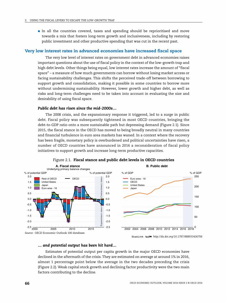
Public debt has risen since the mid-2000s…
The 2008 crisis, and the expansionary response it triggered, led to a surge in public
debt. Fiscal policy was subsequently tightened in most OECD countries, bringing the
debt-to-GDP ratio onto a more sustainable path but depressing demand (Figure 2.1). Since
2015, the fiscal stance in the OECD has moved to being broadly neutral in many countries
and financial turbulence in euro area markets has waned. In a context where the recovery
has been fragile, monetary policy is overburdened and political uncertainties have risen, a
number of OECD countries have announced in 2016 a reconsideration of fiscal policy
initiatives to support growth and increase long-term productive capacities.
… and potential output has been hit hard…
Estimates of potential output per capita growth in the major OECD economies have
declined in the aftermath of the crisis. They are estimated on average at around 1% in 2016,
almost 1 percentage point below the average in the two decades preceding the crisis
(Figure 2.2). Weak capital stock growth and declining factor productivity were the two main
factors contributing to the decline.
Figure 2.1. Fiscal stance and public debt levels in OECD countries
Source: OECD Economic Outlook 100 database.1 2 http://dx.doi.org/10.1787/888933436706
2000 2005 2010 2015-2.5
-2.0
-1.5
-1.0
-0.5
0.0
0.5
1.0
1.5
2.0% of potential GDP
-2.5
-2.0
-1.5
-1.0
-0.5
0.0
0.5
1.0
1.5
2.0% of potential GDP
Con
trac
tion
ary
stan
ceE
xpan
sion
ary
stan
ce
Rest of OECDUnited StatesJapanEuro area - 16
OECD
A. Fiscal stance Underlying primary balance changes
2002 2004 2006 2008 2010 2012 2014 2016 2018
% of GDP
0
50
100
150
200
250% of GDP
Euro area - 16OECDUnited StatesJapan
B. Public debt

2. USING THE FISCAL LEVERS TO ESCAPE THE LOW-GROWTH TRAP
OECD ECONOMIC OUTLOOK, VOLUME 2016 ISSUE 2 © OECD 2016 67
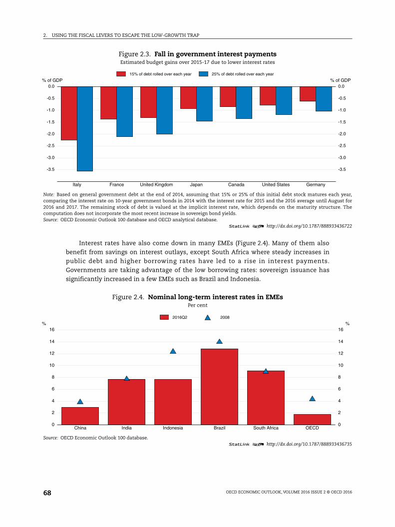
… but lower interest rates provide savings…
The fall in interest rates on government debt in advanced economies has in part
reflected exceptional monetary policy stimulus, with just over 30% of OECD government
debt currently trading at negative yields. This continues a long trend of declining nominal
and real yields over past decades, which has been compounded by very low or even
negative policy rates and large-scale central bank purchases at long maturities, as well as
the reduction in the term premium following changes in banking regulations. In the euro
area, declining risk spreads since the 2011-12 crisis have contributed to lower borrowing
costs. At the same time, many governments have used the opportunity to extend the
maturity of outstanding debt, locking in low rates (OECD, 2016). Nominal yields are also at
relatively low levels in many EMEs compared with past experience, while EME interest
rates remain typically well above those in advanced economies, commensurate with their
growth and inflation prospects.
Declining interest rates have resulted in unexpected savings on interest costs for
governments. Looking forward, and partially accounting for the maturity structure of
public debt, further reduction in interest costs are likely if yields remain around the current
level as old debt at higher yields matures. This would lead to significant additional savings,
notably in Italy and to a lesser extent in France and the United Kingdom over the period
2015-17, under the assumption that 15% of the initial stock of debt is rolled over each year
and the rest is valued at an implicit rate that captures the maturity structure of the debt
(Figure 2.3). Assuming an alternative scenario of 25% of debt maturing each year would
lead to even stronger gains.
Figure 2.2. OECD Potential output growth has slowed markedlyContribution to potential per capita growth
Note: Assuming potential output (Y*) can be represented by a Cobb-Douglas production function in terms of potential employment (N*),the capital stock (K) and total factor productivity (E*) then y* = a * (n*+e*) + (1 - a) * k, where lower case letters denote logs and a is the wageshare. If P is the total population and PWA the population of working age (here taken to be aged 15-74), then the growth rate of potentialGDP per capita (where growth rates are denoted by the first difference, d( ), of logged variables) can be decomposed into the fourcomponents depicted in the figure: d(y* - p) = a * d(e*) + (1-a) * d(k - n*) + d(n* - pwa) + d(pwa - p).1. Potential employment rate refers to potential employment as a share of the working-age population (aged 15-74).2. Active population rate refers to the share of the population of working age in the total population.3. Percentage changes. With growth in Ireland in 2015 computed using gross value added at constant prices excluding foreign-owned
multinational enterprise dominated sectors.Source: OECD Economic Outlook 100 database.
1 2 http://dx.doi.org/10.1787/888933436717
1998 2000 2002 2004 2006 2008 2010 2012 2014 2016 2018-0.5
0.0
0.5
1.0
1.5
2.0
2.5% pts
-0.5
0.0
0.5
1.0
1.5
2.0
2.5% pts
Capital per worker TFPPotential employment rate¹Active population rate²
Potential per capita growth³
2. USING THE FISCAL LEVERS TO ESCAPE THE LOW-GROWTH TRAP
OECD ECONOMIC OUTLOOK, VOLUME 2016 ISSUE 2 © OECD 201668
Interest rates have also come down in many EMEs (Figure 2.4). Many of them also
benefit from savings on interest outlays, except South Africa where steady increases in
public debt and higher borrowing rates have led to a rise in interest payments.
Governments are taking advantage of the low borrowing rates: sovereign issuance has
significantly increased in a few EMEs such as Brazil and Indonesia.
Figure 2.3. Fall in government interest paymentsEstimated budget gains over 2015-17 due to lower interest rates
Note: Based on general government debt at the end of 2014, assuming that 15% or 25% of this initial debt stock matures each year,comparing the interest rate on 10-year government bonds in 2014 with the interest rate for 2015 and the 2016 average until August for2016 and 2017. The remaining stock of debt is valued at the implicit interest rate, which depends on the maturity structure. Thecomputation does not incorporate the most recent increase in sovereign bond yields.Source: OECD Economic Outlook 100 database and OECD analytical database.
1 2 http://dx.doi.org/10.1787/888933436722
Italy France United Kingdom Japan Canada United States Germany
-3.5
-3.0
-2.5
-2.0
-1.5
-1.0
-0.5
0.0% of GDP
-3.5
-3.0
-2.5
-2.0
-1.5
-1.0
-0.5
0.0% of GDP
15% of debt rolled over each year 25% of debt rolled over each year
Figure 2.4. Nominal long-term interest rates in EMEsPer cent
Source: OECD Economic Outlook 100 database.1 2 http://dx.doi.org/10.1787/888933436735
China India Indonesia Brazil South Africa OECD0
2
4
6
8
10
12
14
16%
0
2
4
6
8
10
12
14
16%
2016Q2 2008

2. USING THE FISCAL LEVERS TO ESCAPE THE LOW-GROWTH TRAP
OECD ECONOMIC OUTLOOK, VOLUME 2016 ISSUE 2 © OECD 2016 69
… and fiscal space has increased
Several approaches to measure fiscal space
With conventional monetary policy facing constraints and evidence pointing to a
greater effectiveness of fiscal policy to stabilise the economy than in the past, fiscal space
needs to be reassessed (Furman, 2016). At first glance, fiscal space appears to be a relatively
intuitive concept and can be defined as the “room in a government's budget that allows it
to provide resources for a desired purpose without jeopardizing the sustainability of its
financial position or the stability of the economy” (Heller, 2005).
However, there is no consensus on the way fiscal space should be measured. On one
side, there is uncertainty about the extent to which the government is facing the risk to be
unable to roll over debt anymore. The fiscal space can be thought of as the difference
between the current debt level and the debt limit at which the government would lose
market access. On the other side, fiscal space can be defined in terms of long-term fiscal
sustainability. In practice, the conclusions from these two approaches can differ. For
instance, a country with an expected marked rise in public spending on ageing and health
can have fiscal space according to the former approach, but none according to the latter.
These two aspects of fiscal space are sometimes interrelated, as long-term sustainability
considerations often affect market access through risk premia. However, it is difficult to
comprehensively capture all the factors affecting fiscal space with a single method, and
therefore empirical studies usually predominantly focus on either market access or
long-term sustainability (Figure 2.5).
The absence of information on factors potentially triggering a default in advanced
economies in recent history renders the estimation of fiscal space – not least by the market
access definition – challenging. Quantitative analysis can only build on assumptions on
how households and businesses would react in the future should higher debt levels be
reached. As a result, debt limits and resulting fiscal space estimates should be used with
Figure 2.5. Different approaches to measuring fiscal space
debt limit(probability of default)
actual debt
MARKET ACCESS(ability to roll over debt)
spendingvs.
maximum revenues
actual debt
SUSTAINABILITY(ability to service debt)
FISCAL SPACE
interest rates
(risk-free & market)
potential output growth
fiscal track record &
reaction to debt
macro shocks
spending projections
structural reforms

2. USING THE FISCAL LEVERS TO ESCAPE THE LOW-GROWTH TRAP
OECD ECONOMIC OUTLOOK, VOLUME 2016 ISSUE 2 © OECD 201670
care and uncertainties surrounding such estimates underlined. In real life, debt limits have
to account for many factors, including the level and trajectory of public debt, financing
needs, fiscal track record, economic development, market sentiment and macroeconomic
shocks. However, as statistical methods usually have to be parsimonious, the best option is
to rely on a range on methods to get a full assessment. Rather than pointing to a precise
point estimate, these complementary analyses help in understanding the key mechanisms
at work.
In recent years, a number of new methods have complemented the more traditional
approaches to assess fiscal space. This chapter relies essentially on three (see Annex 2.A1
for an overview of the different methods used in this chapter), with the objective of
approaching the complex reality from different angles:
● Ghosh et al. (2013) and Fournier and Fall (2015) focus on market access. They calculate fiscal
space as the distance between actual debt levels and their estimated limits, measured as
the debt level at which a sovereign borrower loses market access and hence cannot service
its debt in a normal way. Debt limits depend on assumptions made on risk-free interest
rates and potential output growth, the size of shocks that hit economies, the country's
fiscal track record and the fiscal reaction to increasing debt. The fiscal reaction relies on
the assumption that governments cannot indefinitely sustain public primary surpluses
and will experience fiscal fatigue at some point. The model includes a non-linear risk
premium that rises sharply if debt becomes close to the debt limit.
● Bi (2011) and Bi and Leeper (2013) examine sovereign default risks but account for long-term
fiscal sustainability. They rely on a DSGE approach, whereby the shape of the Laffer curve
(which derives expected tax revenues from tax rates) depends on macroeconomic
circumstances. Shocks to the economy and long-term projections of spending and
transfers are accounted for. The approach does not compute a point estimate of the debt
limit, but its distribution, i.e. the probability for a country to default at each value of the
debt-to-GDP ratio. This distribution is derived using the expected present value of future
maximum primary surpluses, where the latter comes from driving tax revenues to the
peak of the Laffer curve and expenditure to its projected level.
● Blanchard et al. (1990) focus essentially on long-term fiscal sustainability in the context
where the interest rate is above the economic growth rate. When the interest rate is
persistently below the growth rate, governments are able to run permanent deficits of any
size. When the differential between the interest rate and growth is positive, fiscal space is
computed as the tax gap between the sustainable and the current tax-to-GDP rate, where
the former is the constant tax rate that would achieve an unchanged debt-to-GDP ratio
over the relevant horizon, for a given projection of public spending and transfers. In this
chapter, a variant of this methodology is used: sustainable tax rates are recomputed using
the FM model (see Annex 2.A2), whereby part of health spending is categorised as an
investment.
The three methods used have their limitations. The market access method assumes
that a lender of last resort prevents any self-fulfilling crisis. In practice, institutions do not
always guarantee this, and a self-fulfilling crisis can crucially depend on other parameters,
such as the debt maturity structure and the share of debt issued in foreign currency. The
approach based on Laffer curves does not take into account possible political economy
considerations associated with driving tax revenues to the peak of the Laffer curve or with
adjusting government spending instead. The approach based on Blanchard et al. (1990), on
2. USING THE FISCAL LEVERS TO ESCAPE THE LOW-GROWTH TRAP
OECD ECONOMIC OUTLOOK, VOLUME 2016 ISSUE 2 © OECD 2016 71
the other hand, does not take macroeconomic shocks into account. Therefore, this chapter
does not rely on any one single approach, but rather treats them as illustrative.
Consequently, the main focus of the analysis is not on precise numerical estimates of fiscal
space, but rather on the trends and underlying mechanism at work.
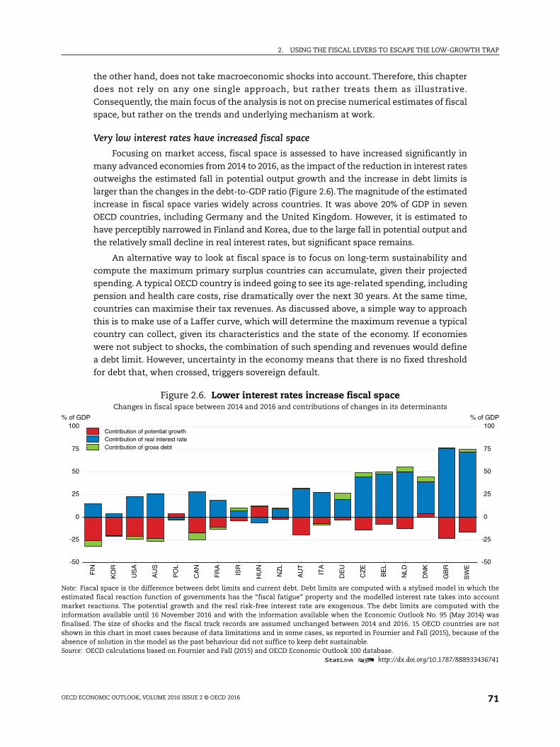
Very low interest rates have increased fiscal space
Focusing on market access, fiscal space is assessed to have increased significantly in
many advanced economies from 2014 to 2016, as the impact of the reduction in interest rates
outweighs the estimated fall in potential output growth and the increase in debt limits is
larger than the changes in the debt-to-GDP ratio (Figure 2.6). The magnitude of the estimated
increase in fiscal space varies widely across countries. It was above 20% of GDP in seven
OECD countries, including Germany and the United Kingdom. However, it is estimated to
have perceptibly narrowed in Finland and Korea, due to the large fall in potential output and
the relatively small decline in real interest rates, but significant space remains.
An alternative way to look at fiscal space is to focus on long-term sustainability and
compute the maximum primary surplus countries can accumulate, given their projected
spending. A typical OECD country is indeed going to see its age-related spending, including
pension and health care costs, rise dramatically over the next 30 years. At the same time,
countries can maximise their tax revenues. As discussed above, a simple way to approach
this is to make use of a Laffer curve, which will determine the maximum revenue a typical
country can collect, given its characteristics and the state of the economy. If economies
were not subject to shocks, the combination of such spending and revenues would define
a debt limit. However, uncertainty in the economy means that there is no fixed threshold
for debt that, when crossed, triggers sovereign default.
Figure 2.6. Lower interest rates increase fiscal spaceChanges in fiscal space between 2014 and 2016 and contributions of changes in its determinants
Note: Fiscal space is the difference between debt limits and current debt. Debt limits are computed with a stylised model in which theestimated fiscal reaction function of governments has the “fiscal fatigue” property and the modelled interest rate takes into accountmarket reactions. The potential growth and the real risk-free interest rate are exogenous. The debt limits are computed with theinformation available until 16 November 2016 and with the information available when the Economic Outlook No. 95 (May 2014) wasfinalised. The size of shocks and the fiscal track records are assumed unchanged between 2014 and 2016. 15 OECD countries are notshown in this chart in most cases because of data limitations and in some cases, as reported in Fournier and Fall (2015), because of theabsence of solution in the model as the past behaviour did not suffice to keep debt sustainable.Source: OECD calculations based on Fournier and Fall (2015) and OECD Economic Outlook 100 database.
1 2 http://dx.doi.org/10.1787/888933436741
-50
-25
0
25
50
75
100% of GDP
-50
-25
0
25
50
75
100% of GDP
FIN
KO
R
US
A
AU
S
PO
L
CA
N
FR
A
ISR
HU
N
NZ
L
AU
T
ITA
DE
U
CZ
E
BE
L
NLD
DN
K
GB
R
SW
E
Contribution of potential growthContribution of real interest rate Contribution of gross debt

2. USING THE FISCAL LEVERS TO ESCAPE THE LOW-GROWTH TRAP
OECD ECONOMIC OUTLOOK, VOLUME 2016 ISSUE 2 © OECD 201672
Looking at fiscal space from this perspective, the distribution probability functions of
the debt limits, that show the respective probability of default at a given level of public debt
for each economy, suggest that most large advanced economies have fiscal space, Japan
being a notable exception. The “market access” approach also suggests that Japan lacks
fiscal space.
The “long-term fiscal sustainability” approach also points to uncertainties regarding
the extent of fiscal space in France and Italy (Figure 2.7). In France, the “market access”
measure of fiscal space points to small gains of fiscal space, within the margin of
uncertainty. The “fiscal sustainability” measure does not send a clear signal either. In Italy,
fiscal space appears to be limited when focusing on fiscal sustainability as compared to
market access, reflecting whether the focus is on past developments of the primary
balance (“market access” approach) or on the budgetary implications of population ageing
(“long-term fiscal sustainability” approach).
A qualitative assessment suggests that the extent of the increase in fiscal space is
mixed across EMEs, even though public debt is lower in these countries than in the average
OECD country. Given the projected output growth, the current interest rate level but also
financial-market fragility, the Economic Outlook projections suggest that there is ample
though narrowing fiscal space in China, while India, Brazil and South Africa will continue
to lack fiscal space in the absence of reforms.
Figure 2.7. Fiscal limit cumulative distribution functions
Note: For each country the curve depicts the probability of default at each given public debt-to GDP level. For instance,the probability of default is zero is in all advanced economies countries when the actual debt-to-GDP ratio is below113%. Circles correspond to the 2015 level of the debt-to-GDP ratio. Public debt refers to general government grossfinancial liabilities according to the SNA definition.Source: OECD calculations using Bi (2011) and Bi and Leeper (2013).
0
0,2
0,4
0,6
0,8
1
70 83 95 108 121 133 146 158 171 183
United States Japan Germany FranceItaly United Kingdom Canada
debt-GDP
Japan: 230 % Japan: 230 %
2. USING THE FISCAL LEVERS TO ESCAPE THE LOW-GROWTH TRAP
OECD ECONOMIC OUTLOOK, VOLUME 2016 ISSUE 2 © OECD 2016 73
Fiscal space depends on the pace at which real interest rates and potential output growth become aligned…
Low interest rates provide policy makers with room for manoeuvre but are also
associated with fiscal risks. Assuming the differentials between growth and interest rates
gradually converge to their long-term average, the long-term measure of fiscal space, based
on Blanchard et al. (1990) and OECD pension spending projections, point to limited
sustainability risks over the long term in the three main euro area economies (OECD,
2015a). However, health spending is expected to rise markedly over the next decades as the
population ages (de la Maisonneuve and Oliveira Martins, 2015). Accounting for these
projected increases in health costs, large advanced economies will have to adjust their tax
ratios and/or spending by several percentage points of GDP to stabilise debt at current
levels by 2060. The pace of this adjustment will depend to a large extent on the speed at
which real interest rates become aligned to output growth. Locking in the very low levels of
interest rates by issuing more long-dated bonds would help manage the interest-rate risk.
… but structural reforms to key spending programmes can help increase fiscal space
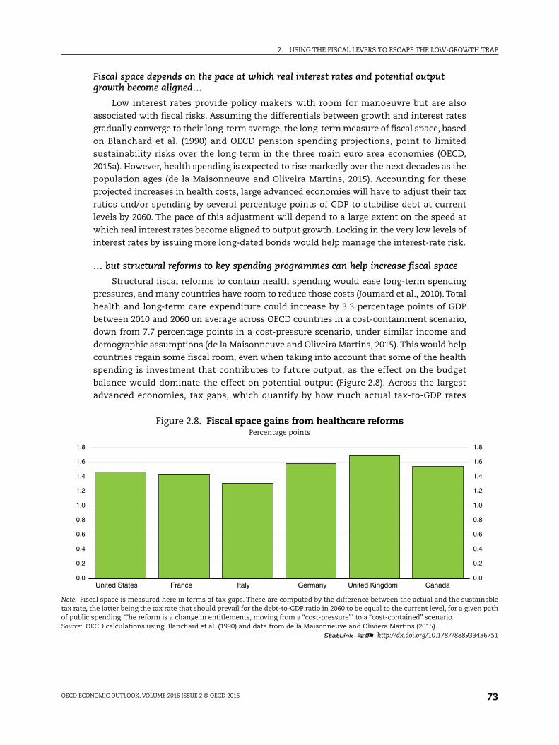
Structural fiscal reforms to contain health spending would ease long-term spending
pressures, and many countries have room to reduce those costs (Joumard et al., 2010). Total
health and long-term care expenditure could increase by 3.3 percentage points of GDP
between 2010 and 2060 on average across OECD countries in a cost-containment scenario,
down from 7.7 percentage points in a cost-pressure scenario, under similar income and
demographic assumptions (de la Maisonneuve and Oliveira Martins, 2015). This would help
countries regain some fiscal room, even when taking into account that some of the health
spending is investment that contributes to future output, as the effect on the budget
balance would dominate the effect on potential output (Figure 2.8). Across the largest
advanced economies, tax gaps, which quantify by how much actual tax-to-GDP rates
Figure 2.8. Fiscal space gains from healthcare reformsPercentage points
Note: Fiscal space is measured here in terms of tax gaps. These are computed by the difference between the actual and the sustainabletax rate, the latter being the tax rate that should prevail for the debt-to-GDP ratio in 2060 to be equal to the current level, for a given pathof public spending. The reform is a change in entitlements, moving from a “cost-pressure”' to a “cost-contained” scenario.Source: OECD calculations using Blanchard et al. (1990) and data from de la Maisonneuve and Oliviera Martins (2015).
1 2 http://dx.doi.org/10.1787/888933436751
0.0
0.2
0.4
0.6
0.8
1.0
1.2
1.4
1.6
1.8
0.0
0.2
0.4
0.6
0.8
1.0
1.2
1.4
1.6
1.8
United States France Italy Germany United Kingdom Canada

2. USING THE FISCAL LEVERS TO ESCAPE THE LOW-GROWTH TRAP
OECD ECONOMIC OUTLOOK, VOLUME 2016 ISSUE 2 © OECD 201674
would have to increase for the debt-to-GDP ratios to be stabilised at current levels over the
long term, would be reduced by 1.5 points on average.
Thanks to a number of past reforms of pension systems, long-run sustainability has
improved in some countries. Further reforms in this direction will also raise fiscal space.
Whereas low growth of aggregate productivity can add to pension sustainability pressures
(see Chapter 1), reforms that increase the retirement age allow contribution rates and
replacement rates to be maintained, while also contributing to sizeable output gains
(Johansson and Fournier, 2016). Finally, by raising potential output, product and labour
market reforms will also increase the fiscal space available to governments.
A fiscal initiative can help boost long-term growth and inclusivenessA continuation of the very low economic growth in recent years would further
undermine longer-term fiscal sustainability and accentuates the need for well-designed
fiscal stimulus programmes to raise productive potential. Such a programme could include
high-quality spending on education, health and research and development as well as green
infrastructure that all bring significant output gains in the long run and foster
inclusiveness. The question is to what extent such a stimulus could be financed by issuing
long-term bonds, without endangering long-term fiscal sustainability.
This section reviews the likely impact of such an initiative both in the short and long
term. It also identifies the factors that can help maximise the growth impact of such an
initiative. Those impacts will vary over time (Figure 2.9). Indeed, high returns on capital,
the persistence of long-term unemployment and the implementation of structural reforms
will have an impact that increases over time, while the effect of acting collectively and of
financing the initiative through higher public deficit in the short term will dissipate over
time. These different factors are described in more details in the following sections.
Figure 2.9. Factors that can influence the growth impact of a fiscal initiative
Note: The figure is illustrative and the relative gains of individual factors and the timing of their gains are not drawnto scale.
Fiscal initiative
Deficit-financing Return on
public capital
Long-term unemployment
Structural reforms Collective action
Short-term Time
Output gains
Long-term
2. USING THE FISCAL LEVERS TO ESCAPE THE LOW-GROWTH TRAP
OECD ECONOMIC OUTLOOK, VOLUME 2016 ISSUE 2 © OECD 2016 75
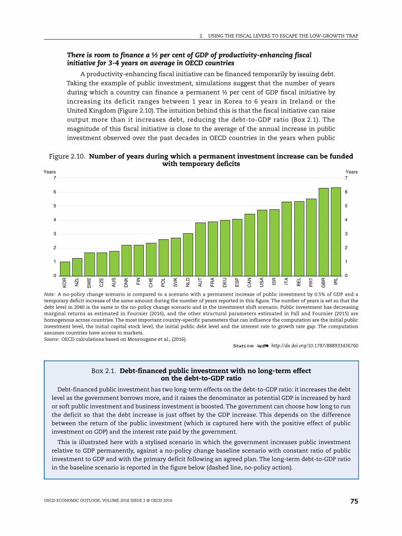
There is room to finance a ½ per cent of GDP of productivity-enhancing fiscalinitiative for 3-4 years on average in OECD countries
A productivity-enhancing fiscal initiative can be financed temporarily by issuing debt.
Taking the example of public investment, simulations suggest that the number of years
during which a country can finance a permanent ½ per cent of GDP fiscal initiative by
increasing its deficit ranges between 1 year in Korea to 6 years in Ireland or the
United Kingdom (Figure 2.10). The intuition behind this is that the fiscal initiative can raise
output more than it increases debt, reducing the debt-to-GDP ratio (Box 2.1). The
magnitude of this fiscal initiative is close to the average of the annual increase in public
investment observed over the past decades in OECD countries in the years when public
Figure 2.10. Number of years during which a permanent investment increase can be fundedwith temporary deficits
Note: A no-policy change scenario is compared to a scenario with a permanent increase of public investment by 0.5% of GDP and atemporary deficit increase of the same amount during the number of years reported in this figure. The number of years is set so that thedebt level in 2040 is the same in the no-policy change scenario and in the investment shift scenario. Public investment has decreasingmarginal returns as estimated in Fournier (2016), and the other structural parameters estimated in Fall and Fournier (2015) arehomogenous across countries. The most important country-specific parameters that can influence the computation are the initial publicinvestment level, the initial capital stock level, the initial public debt level and the interest rate to growth rate gap. The computationassumes countries have access to markets.Source: OECD calculations based on Mourougane et al., (2016).
1 2 http://dx.doi.org/10.1787/888933436760
Box 2.1. Debt-financed public investment with no long-term effecton the debt-to-GDP ratio
Debt-financed public investment has two long-term effects on the debt-to-GDP ratio: it increases the debtlevel as the government borrows more, and it raises the denominator as potential GDP is increased by hardor soft public investment and business investment is boosted. The government can choose how long to runthe deficit so that the debt increase is just offset by the GDP increase. This depends on the differencebetween the return of the public investment (which is captured here with the positive effect of publicinvestment on GDP) and the interest rate paid by the government.
This is illustrated here with a stylised scenario in which the government increases public investmentrelative to GDP permanently, against a no-policy change baseline scenario with constant ratio of publicinvestment to GDP and with the primary deficit following an agreed plan. The long-term debt-to-GDP ratioin the baseline scenario is reported in the figure below (dashed line, no-policy action).
0
1
2
3
4
5
6
7Years
0
1
2
3
4
5
6
7Years
KO
R
NZ
L
SW
E
CZ
E
AU
S
DN
K
FIN
CH
E
PO
L
SV
K
NLD
AU
T
FR
A
DE
U
ES
P
CA
N
US
A
ISR
ITA
BE
L
PR
T
GB
R
IRL

2. USING THE FISCAL LEVERS TO ESCAPE THE LOW-GROWTH TRAP
OECD ECONOMIC OUTLOOK, VOLUME 2016 ISSUE 2 © OECD 201676
Box 2.1. Debt-financed public investment with no long-term effecton the debt-to-GDP ratio (cont.)
In a first scenario, it is assumed that public investment is financed by cuts in current spending or by taxincreases. In this scenario, public borrowing is unchanged, while the denominator is increased on accountof the different multipliers on the investment versus current spending versus taxes: the debt-to-GDP ratiodeclines. As a result, the debt-to-GDP ratio is 2 percentage points below the no-policy action scenario(triangle in the figure below). In a second scenario, investment is deficit-financed for a given number ofyears, and government borrowing will increase with the number of years, as illustrated by the solid line inthe figure below. In this second scenario, it is assumed that it takes time to restrain current spending or toreap the benefits of public investment in terms of higher tax revenues. As the figure illustrates, there is abreak-even duration of investment for which the debt-to-GDP ratio is equal to the one with the no-policychange scenario (circle in the figure below).
This break-even number of years depends on the effect of public investment on potential GDP. Should thegovernment identify higher-quality projects and activities, the number of years of deficit-financing couldbe even greater. This is most likely the case in countries where public investment decreased during thecrisis, or where the public capital stock is relatively low. Structural reforms that increase GDP can alsoprovide room for longer-lasting deficits. Last, the break-even number of years depends on the level of thedebt-to-GDP ratio itself: it is all the more crucial that the portfolio of changes to the fiscal budget increasesGDP in the most indebted countries. For instance, a policy that increases GDP by one per cent while leavingthe debt level unchanged would decrease the debt-to-GDP ratio by one percentage point if the debt-to-GDPratio is 100%; it would decrease the debt-to-GDP ratio by only one-half of a percentage point if the debt-to-GDPratio is 50%.
This stylised exercise considers gross debt: it ignores public real assets. This is a prudent simplification:the number of years during which investment-led stimulus can be deficit-financed would be higher if onereplaces gross debt by net debt in the analysis. A permanent increase in public investment implies apermanent increase in the capital stock that decreases net debt.
The break-even number of years of deficit-financed public investment:the example of Germany
Long-term public debt in per cent of GDP
Note: The 2040 debt-to-GDP ratio is reported here to represent the long-term debt-to-GDP ratio.Source: OECD calculations based on Fall and Fournier (2015).
1 2 http://dx.doi.org/10.1787/888933436694
0 1 2 3 4 5 6 755
56
57
58
59
60
61
62
55
56
57
58
59
60
61
62
No policy action
Number of years during which the investment shock is deficit-financed (solid line)
Public investment shock without deficit
Break-even number of years
Public investment shock

2. USING THE FISCAL LEVERS TO ESCAPE THE LOW-GROWTH TRAP
OECD ECONOMIC OUTLOOK, VOLUME 2016 ISSUE 2 © OECD 2016 77
investment increased (0.6 % of GDP). In the simulation, the number of years is calculated so
that the public debt level remained unchanged in 2040. This number is a function of the
country's initial level of the public capital stock and of the differential between economic
growth and the interest rate, as well as the initial level of public debt. According to this
analysis, Japan is found to have no room to finance a fiscal initiative through higher deficit.
A productivity-enhancing fiscal initiative boosts the economy in the short and thelong term
A productivity-enhancing fiscal initiative has not only a short-term demand effect but
also a longer-term supply effect, in contrast with boosting current public expenditure.
Public investment is an example of such a fiscal measure. To the extent that monetary
policy is constrained, an investment-led stimulus may raise output more than it increases
debt, leading to a fall in the debt-to-GDP ratio in the short term. This will likely be the case
if public investment manages to catalyse private investment. In the long term, the boost in
investment increases the productive capacity of the economy and the positive effect on
potential output leads in additional tax revenues. Whether higher investment increases or
lowers the debt-to-GDP ratio in the long term will depend on a number of factors, including
the extent to which potential output is boosted. In all cases, the long-term effect of a public
investment shock on the debt ratio will be more favourable than a public consumption
shock that does not raise the productive capacity of economies.
Strong institutions and effective public governance are key for a successful fiscal
initiative. This includes respect for the rule of law, quality regulation, transparency,
openness and integrity. Whole-of-government approaches will improve outcomes and
enhance the use of public resources. Fiscal policy is intertwined with a lot of other public
policies – like competitiveness, climate-change mitigation, managing demographic change
and innovation – and their effective combination can bring about synergies (OECD, 2015b).
Regarding public investment specifically, good governance and reliable ex ante assessment
of projects’ social rates of return are crucial to ensure that high returns materialise and to
prevent the cost overruns and over-estimation of future demand that have occurred in a
number of past infrastructure projects (Persson and Song, 2010). More generally, regulation
and other framework conditions, including access to markets and pricing regimes, will also
affect the return on investment (Sutherland et al., 2011). Evidence suggests that most OECD
countries still have room to improve their existing regulatory framework to ensure that
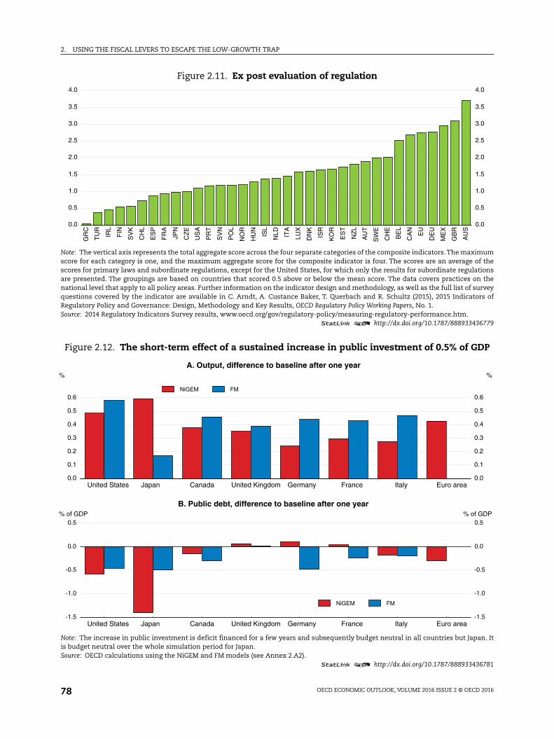
regulation is fit for purpose and achieves its goals (Figure 2.11, OECD, 2015c).
The short-term output impact of ½ per cent of GDP fiscal initiative could be up to 0.6% in the first year…
Quantitatively, in the current environment and with monetary policy unchanged, a
permanent investment-led stimulus of ½ percentage point of GDP that would be
deficit-financed for a few years is estimated to increase output by 0.4-0.6% in the first year in
the large advanced economies (Figure 2.12). However, short-term output gains are particularly
unclear for Japan where the evidence points to lower and much more uncertain fiscal
multipliers in the most recent period (Auerbach and Gorodnichenko, 2014). In this country, the
fiscal initiative is assumed to be budget neutral over the whole simulation period.
Estimates have been computed using three models (Annex 2.A2). They assume
projects undertaken are economically worthwhile and can be implemented without delay.
While some infrastructure projects may take a long time to activate, other forms of public
2. USING THE FISCAL LEVERS TO ESCAPE THE LOW-GROWTH TRAP
OECD ECONOMIC OUTLOOK, VOLUME 2016 ISSUE 2 © OECD 201678
Figure 2.11. Ex post evaluation of regulation
Note: The vertical axis represents the total aggregate score across the four separate categories of the composite indicators. The maximumscore for each category is one, and the maximum aggregate score for the composite indicator is four. The scores are an average of thescores for primary laws and subordinate regulations, except for the United States, for which only the results for subordinate regulationsare presented. The groupings are based on countries that scored 0.5 above or below the mean score. The data covers practices on thenational level that apply to all policy areas. Further information on the indicator design and methodology, as well as the full list of surveyquestions covered by the indicator are available in C. Arndt, A. Custance Baker, T. Querbach and R. Schultz (2015), 2015 Indicators ofRegulatory Policy and Governance: Design, Methodology and Key Results, OECD Regulatory Policy Working Papers, No. 1.Source: 2014 Regulatory Indicators Survey results, www.oecd.org/gov/regulatory-policy/measuring-regulatory-performance.htm.
1 2 http://dx.doi.org/10.1787/888933436779
Figure 2.12. The short-term effect of a sustained increase in public investment of 0.5% of GDP
Note: The increase in public investment is deficit financed for a few years and subsequently budget neutral in all countries but Japan. Itis budget neutral over the whole simulation period for Japan.Source: OECD calculations using the NiGEM and FM models (see Annex 2.A2).
1 2 http://dx.doi.org/10.1787/888933436781
0.0
0.5
1.0
1.5
2.0
2.5
3.0
3.5
4.0
0.0
0.5
1.0
1.5
2.0
2.5
3.0
3.5
4.0G
RC
TU
R
IRL
FIN
SV
K
CH
L
ES
P
FR
A
JPN
CZ
E
US
A
PR
T
SV
N
PO
L
NO
R
HU
N
ISL
NLD IT
A
LUX
DN
K
ISR
KO
R
ES
T
NZ
L
AU
T
SW
E
CH
E
BE
L
CA
N
EU
DE
U
ME
X
GB
R
AU
S
0.0
0.1
0.2
0.3
0.4
0.5
0.6
%
0.0
0.1
0.2
0.3
0.4
0.5
0.6
%
United States Japan Canada United Kingdom Germany France Italy Euro area
NiGEM FM
A. Output, difference to baseline after one year
-1.5
-1.0
-0.5
0.0
0.5% of GDP
-1.5
-1.0
-0.5
0.0
0.5% of GDP
United States Japan Canada United Kingdom Germany France Italy Euro area
NiGEM FM
B. Public debt, difference to baseline after one year
2. USING THE FISCAL LEVERS TO ESCAPE THE LOW-GROWTH TRAP
OECD ECONOMIC OUTLOOK, VOLUME 2016 ISSUE 2 © OECD 2016 79
investment could be mobilised more rapidly and, given the recent falls in public
investment in many countries, there may be a backlog of existing projects or maintenance
needs. Furthermore, commitment to bring new projects on stream may help to improve the
environment for private investment.
Raising public investment lifts business investment by a median of 0.7% in the most
advanced economies after one year, with corresponding increases in the business sector
capital stock and potential output. These effects could be even stronger if the additional
public investment were to be concentrated in network industries, particularly in the
European Union, where there is a greater possibility of crowding in private investment
(OECD, 2015d).
The stimulus impact on the public debt-to-GDP ratio depends essentially on growth
dynamics. The public debt-to-GDP ratio would fall compared to the baseline in the short
term in the United States and, to a lesser extent, in the euro area.
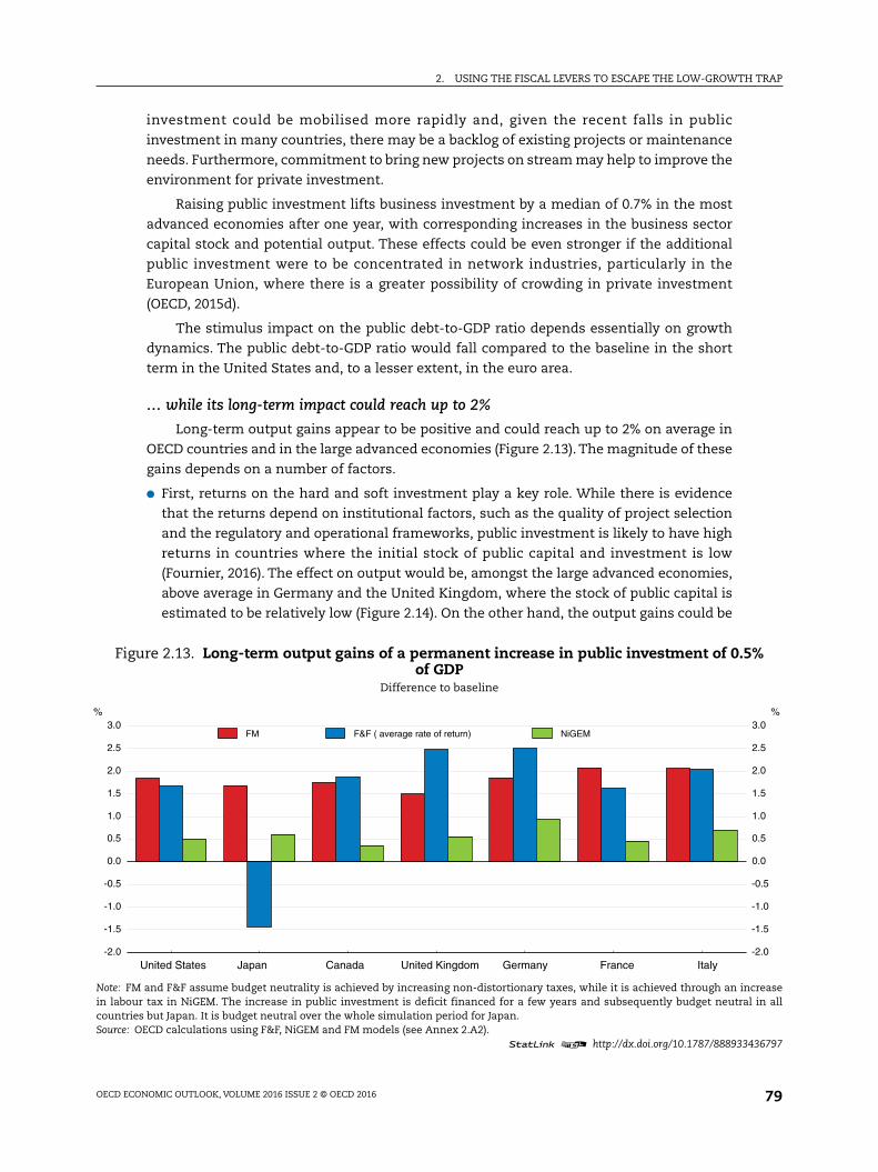
… while its long-term impact could reach up to 2%
Long-term output gains appear to be positive and could reach up to 2% on average in
OECD countries and in the large advanced economies (Figure 2.13). The magnitude of these
gains depends on a number of factors.
● First, returns on the hard and soft investment play a key role. While there is evidence
that the returns depend on institutional factors, such as the quality of project selection
and the regulatory and operational frameworks, public investment is likely to have high
returns in countries where the initial stock of public capital and investment is low
(Fournier, 2016). The effect on output would be, amongst the large advanced economies,
above average in Germany and the United Kingdom, where the stock of public capital is
estimated to be relatively low (Figure 2.14). On the other hand, the output gains could be
Figure 2.13. Long-term output gains of a permanent increase in public investment of 0.5%of GDP
Difference to baseline
Note: FM and F&F assume budget neutrality is achieved by increasing non-distortionary taxes, while it is achieved through an increasein labour tax in NiGEM. The increase in public investment is deficit financed for a few years and subsequently budget neutral in allcountries but Japan. It is budget neutral over the whole simulation period for Japan.Source: OECD calculations using F&F, NiGEM and FM models (see Annex 2.A2).
1 2 http://dx.doi.org/10.1787/888933436797
-2.0
-1.5
-1.0
-0.5
0.0
0.5
1.0
1.5
2.0
2.5
3.0%
-2.0
-1.5
-1.0
-0.5
0.0
0.5
1.0
1.5
2.0
2.5
3.0%
United States Japan Canada United Kingdom Germany France Italy
FM F&F ( average rate of return) NiGEM

2. USING THE FISCAL LEVERS TO ESCAPE THE LOW-GROWTH TRAP
OECD ECONOMIC OUTLOOK, VOLUME 2016 ISSUE 2 © OECD 201680
very negative for Japan, reflecting a large initial public capital stock and associated low
and even negative rates of return at the margin for conventionally-defined public capital.
The long-term elasticity of capital to potential output and the depreciation rates
determine the extent to which the additional public investment will accumulate into
productive capacity. These parameters have been calibrated using results reported in the
economic literature. For instance, a meta-study by Bom and Ligthard (2014) suggests,
that the elasticity of investment in core infrastructure, such as roads, rails and
telecommunications on long-term output could be relatively high. In particular,
spillovers from the higher public capital stock on potential output have been estimated
to be positive for infrastructure spending in the United States and in the European Union
(White House, 2016; European Commission, 2014).
● Second, the long-term impact also depends on the way budget neutrality is achieved
over the medium term. The 2% gains in long-term output are conditional on the
assumption that the stimulus is financed after three to four years through an increase in
non-distortionary taxes or a cut in other spending, with neither of these factors affecting
potential output. Alternative assumptions, such as financing a stimulus through an
increase in direct taxes on households, which reduces household disposable income and
spending, would lower this impact.
Structural reforms enhance the growth impact of the fiscal initiative
The output gains of the fiscal initiative would be increased if countries undertake
much needed structural reforms that will enhance total factor productivity and potential
output. In recent years, the pace of structural reforms in both advanced and EMEs has
slowed. This slowdown is particularly troubling for long-term growth prospects. Actions
across a broad range of reform objectives, such as product market competition, labour
mobility and financial market robustness are essential in order to reverse the widespread
slowdown in productivity and improve inclusiveness.
Figure 2.14. Long-term output gains of different assumptions on the rate of returnon public investment
Difference to baseline
Note: The increase in public investment is deficit financed for a few years and subsequently budget neutral in all countries but Japan. Itis budget neutral over the whole simulation period for Japan.Source: OECD calculations using the F&F models.
1 2 http://dx.doi.org/10.1787/888933436800
-3
-2
-1
0
1
2
3
4
5%
-3
-2
-1
0
1
2
3
4
5%
United States Japan Canada United Kingdom Germany France Italy
F&F ( high rate of return) F&F ( average rate of return) F&F ( low rate of return)
2. USING THE FISCAL LEVERS TO ESCAPE THE LOW-GROWTH TRAP
OECD ECONOMIC OUTLOOK, VOLUME 2016 ISSUE 2 © OECD 2016 81
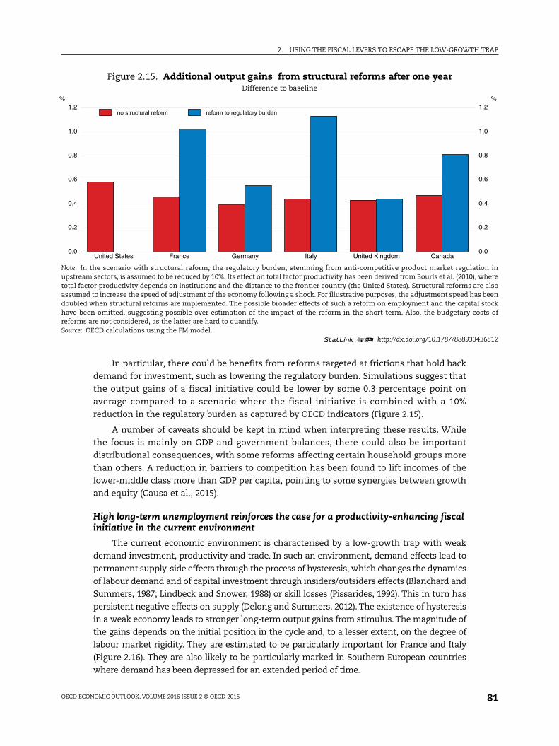
In particular, there could be benefits from reforms targeted at frictions that hold back
demand for investment, such as lowering the regulatory burden. Simulations suggest that
the output gains of a fiscal initiative could be lower by some 0.3 percentage point on
average compared to a scenario where the fiscal initiative is combined with a 10%
reduction in the regulatory burden as captured by OECD indicators (Figure 2.15).
A number of caveats should be kept in mind when interpreting these results. While
the focus is mainly on GDP and government balances, there could also be important
distributional consequences, with some reforms affecting certain household groups more
than others. A reduction in barriers to competition has been found to lift incomes of the
lower-middle class more than GDP per capita, pointing to some synergies between growth
and equity (Causa et al., 2015).
High long-term unemployment reinforces the case for a productivity-enhancing fiscalinitiative in the current environment
The current economic environment is characterised by a low-growth trap with weak
demand investment, productivity and trade. In such an environment, demand effects lead to
permanent supply-side effects through the process of hysteresis, which changes the dynamics
of labour demand and of capital investment through insiders/outsiders effects (Blanchard and
Summers, 1987; Lindbeck and Snower, 1988) or skill losses (Pissarides, 1992). This in turn has
persistent negative effects on supply (Delong and Summers, 2012). The existence of hysteresis
in a weak economy leads to stronger long-term output gains from stimulus. The magnitude of
the gains depends on the initial position in the cycle and, to a lesser extent, on the degree of
labour market rigidity. They are estimated to be particularly important for France and Italy
(Figure 2.16). They are also likely to be particularly marked in Southern European countries
where demand has been depressed for an extended period of time.
Figure 2.15. Additional output gains from structural reforms after one yearDifference to baseline
Note: In the scenario with structural reform, the regulatory burden, stemming from anti-competitive product market regulation inupstream sectors, is assumed to be reduced by 10%. Its effect on total factor productivity has been derived from Bourls et al. (2010), wheretotal factor productivity depends on institutions and the distance to the frontier country (the United States). Structural reforms are alsoassumed to increase the speed of adjustment of the economy following a shock. For illustrative purposes, the adjustment speed has beendoubled when structural reforms are implemented. The possible broader effects of such a reform on employment and the capital stockhave been omitted, suggesting possible over-estimation of the impact of the reform in the short term. Also, the budgetary costs ofreforms are not considered, as the latter are hard to quantify.Source: OECD calculations using the FM model.
1 2 http://dx.doi.org/10.1787/888933436812
United States France Germany Italy United Kingdom Canada0.0
0.2
0.4
0.6
0.8
1.0
1.2%
0.0
0.2
0.4
0.6
0.8
1.0
1.2%
no structural reform reform to regulatory burden

2. USING THE FISCAL LEVERS TO ESCAPE THE LOW-GROWTH TRAP
OECD ECONOMIC OUTLOOK, VOLUME 2016 ISSUE 2 © OECD 201682
Hysteresis matters essentially in the longer term and when the stimulus is sustained
(Mourougane et al., 2016). For instance, an investment-led fiscal stimulus is found to have
a stronger long-term effect on the output level of about ½ percentage point in France and
Italy than it would be in the absence of labour market hysteresis. The differences are
smaller, of by around ¼ percentage point, in the United States and Canada. Starting from
an output gap that is close to zero, the United Kingdom does not benefit from additional
output gains when hysteresis is taken into account.
Collective action brings additional gains
With globalisation and tighter links between countries, collective action may be
increasingly more powerful than taking fiscal action alone. Demand spillovers, whereby
policy action in one country influences investment and export flows with partner
economies (Barrell et al., 2012), are found to be significant in the case of synchronised fiscal
stimulus (Auerbach and Gorodnichenko, 2014). In addition to these traditional channels,
knowledge spillovers, resulting from the international diffusion of innovations and higher
trade levels, will raise the benefits to other countries from higher innovation in each
economy. While the knowledge spillovers are less important in the short term, they play a
role in the long term.
Episodes of collective fiscal action have rarely been observed in the past, the
coordinated response to the 2008 financial crisis and the period of fiscal austerity that
followed in the euro area being two notable exceptions. For example, the number of OECD
countries which simultaneously injected a sustained large public investment stimulus was
around four per year on average in the pre-crisis period, and in general these were not
coordinated. By contrast, more than 15 countries markedly increased public investment
spending in 2008 and 17 did so in 2009.
In order to quantify those spillover effects, the impact of an increase of ½ percentage
point of GDP in public investment for each country acting alone was compared with a
scenario where all the countries act simultaneously in a context where monetary policy is
Figure 2.16. Effects of hysteresis on long-term output gainsDifference to baseline
Source: OECD calculations using the FM model.1 2 http://dx.doi.org/10.1787/888933436821
0.0
0.5
1.0
1.5
2.0
2.5%
0.0
0.5
1.0
1.5
2.0
2.5%
United States Japan France Germany Italy United Kingdom Canada
without hysteresis with hysteresis
2. USING THE FISCAL LEVERS TO ESCAPE THE LOW-GROWTH TRAP
OECD ECONOMIC OUTLOOK, VOLUME 2016 ISSUE 2 © OECD 2016 83
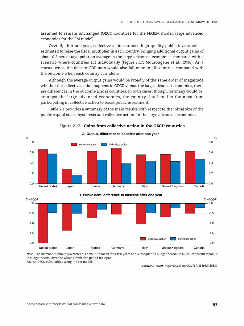
assumed to remain unchanged (OECD countries for the NiGEM model, large advanced
economies for the FM model).
Overall, after one year, collective action to raise high-quality public investment is
estimated to raise the fiscal multiplier in each country, bringing additional output gains of
about 0.2 percentage point on average in the large advanced economies compared with a
scenario where countries act individually (Figure 2.17, Mourougane et al., 2016). As a
consequence, the debt-to-GDP ratio would also fall more in all countries compared with
the outcome when each country acts alone.
Although the average output gains would be broadly of the same order of magnitude
whether the collective action happens in OECD versus the large advanced economies, there
are differences in the outcome across countries. In both cases, though, Germany would be,
amongst the large advanced economies, the country that benefits the most from
participating in collective action to boost public investment.
Table 2.1 provides a summary of the main results with respect to the initial size of the
public capital stock, hysteresis and collective action for the large advanced economies.
Figure 2.17. Gains from collective action in the OECD countries
Note: The increase in public investment is deficit financed for a few years and subsequently budget neutral in all countries but Japan. Itis budget neutral over the whole simulation period for Japan.Source: OECD calculations using the FM model.
1 2 http://dx.doi.org/10.1787/888933436832
0.0
0.2
0.4
0.6
0.8%
0.0
0.2
0.4
0.6
0.8%
United States Japan France Germany Italy United Kingdom Canada
collective action individual action
A. Output, difference to baseline after one year
-2.0
-1.5
-1.0
-0.5
0.0% of GDP
-2.0
-1.5
-1.0
-0.5
0.0% of GDP
United States Japan France Germany Italy United Kingdom Canada
collective action individual action
B. Public debt, difference to baseline after one year

2. USING THE FISCAL LEVERS TO ESCAPE THE LOW-GROWTH TRAP
OECD ECONOMIC OUTLOOK, VOLUME 2016 ISSUE 2 © OECD 201684
The composition of spending and taxes should be made more supportive ofinclusive growth
A fiscal initiative now can be an opportunity to improve the tax and spending mix by
focusing on the measures that will foster long-term growth and promote inclusiveness and
the protection of the environment. Countries where fiscal space is limited also have room
to move toward a mix that is more supportive of inclusive growth. Productive spending has
a permanent effect on the supply side of the economy, while unproductive spending has a
short-lived effect. Likewise, the tax structure can be modified to support inclusive growth.
The composition of the fiscal initiative is thus essential for fiscal expansion to be
undertaken without increasing the debt-to-GDP ratio in the long run.
Boosting public investment and improving education outcomes can yield largegrowth gains and benefit all
Increasing the share of public investment in government spending yields large growth
gains for the whole population (Table 2.2; Fournier, 2016). These gains are particularly
strong in fields that are associated with large externalities, such as health (e.g. hospitals,
medical equipment and prevention). A spending shift towards public investment and away
from other spending in less advanced economies would also speed up their convergence
Table 2.1. Country-specific conditions and the impactof public investment stimulus
Low level of public capital/high rateof return
Hysteresis Collective action
United States + + +
Japan -- = +
Germany ++ = ++
France + ++ +
Italy + ++ +
United Kingdom ++ = +
Canada + + +
Note: signs summarise the amplitude of the output gains following an investment-led stimulus. + means that outputgains are higher, ++ that they are markedly higher and = that there is no change. For instance the existence ofhysteresis in France and Italy makes these countries gain more from such a measure than other advancedeconomies.Source: OECD calculations based on F&F, FM and NiGEM models.
Table 2.2. Effects of public spending reforms on growth and equity
Policy Growth Income of the poorCountries which will benefitthe most from the reform
Increasing government effectiveness + + FRA, GRC, HUN, ITA, SVN
Increasing education outcomes + + CHL, GRC, MEX, PRT, TUR
Increasing public investment (including R&D) + + BEL, DEU, GBR, IRL, ISR, ITA, MEX, TUR
Pension reform + + AUT, DEU, FIN, FRA, GRC, ITA, JPN, POL, PRT, SVN
Increasing family benefits 0 + CHE, ESP, GRC, PRT
Decreasing public subsidies + 0 BEL, CHE
Note: The analysis is based on information up until 2013 and therefore do not reflect recently implemented reforms.+ stands for a positively significant, and – for a negatively significant. The countries which benefit the most from thereform are those where reforms would yield gains of more than 10% of GDP. For family benefits, the table showscountries where the reform would increase the income of the poor by more than 20%.Source: Fournier J.M. and Johansson A. (2016), “The Effect of the Size and the Mix of Public Spending on Growth andInequality”, OECD Economics Department Working Papers, No. 1344.

2. USING THE FISCAL LEVERS TO ESCAPE THE LOW-GROWTH TRAP
OECD ECONOMIC OUTLOOK, VOLUME 2016 ISSUE 2 © OECD 2016 85
with the most advanced economies, provided that good governance is in place. As
discussed above, the growth gains from increasing public investment may decline at a high
level of the public capital stock due to decreasing returns. Still, estimations suggest that all
OECD countries but Japan have room for additional public investment. Overall, such a
spending shift would lift “all boats” as it raises average income without any adverse equity
effects. Targeted additional capital spending can also help achieve long-term objectives
such as those related to climate change and environmental quality.
Output gains from increased public spending on research and development are
potentially large, particularly if spending is directed to basic research where widespread
market failures lead to under-investment by the private sector (OECD, 2015c). Higher public
spending on basic research can also enhance the ability of economies to learn from
innovations at the global frontier (Saia et al., 2015).
Recent evidence based on OECD countries suggests that increasing the quality of, and
the time spent in, education yields large growth gains by raising skills and thereby
productivity (Fournier and Johansson, 2016). In addition, an education reform that aims at
encouraging completion of secondary education can decrease income inequality. This is in
line with earlier research on the effect of education on earnings inequality: an increase in
the share of upper-secondary degrees decreases labour earning inequality, while an
increase in the share of tertiary degrees increases inequality in education outcomes and
hence can increase earnings inequality (Fournier and Koske, 2012).
Shifting spending towards family benefits and childcare and away from other
spending also decreases income inequality. This may also facilitate the participation of
second earners in the labour market and will help the social inclusion of children from more
deprived backgrounds. In the long run, these spending reforms could be funded by cutting
public subsidies and raising the retirement age, as pensions and subsidies can have adverse
effects on growth. Subsidy cuts that yield disproportionately greater gains for the rich than
the poor can be complemented by other redistributive policies that reduce inequality.
Turning to revenues, shifting part of the revenue base from personal and corporate
income taxes to less distortive taxes such as recurrent taxes on immovable property or
consumption would boost growth (Johansson et al., 2008; Table 2.3). However, such a tax
shift would reduce the overall progressivity of the tax system as these taxes are less
progressive than income taxes. Furthermore, a combination of base broadening and rate
reduction of individual taxes can complement a revenue shift.
Table 2.3. Growth and equity effects of decreases in selected tax and contributions
Decrease in…Growth Equity
Short-term Long-term Short-term Long-term
Personal income taxes + ++ - -
Social security contributions + ++ + +
Corporate income taxes + ++ - -
Environmental taxes + - +
Consumption taxes (other than environmental) + + +
Recurrent taxes on immovable property +
Other property taxes + -- -
Sales of goods and services + - + +
Source: Cournède, B., A. Pina and A. Goujard (2014), “Reconciling Fiscal Consolidation with Growth and Equity”, OECDJournal: Economic Studies, Vol. 2013 Issue 1.

2. USING THE FISCAL LEVERS TO ESCAPE THE LOW-GROWTH TRAP
OECD ECONOMIC OUTLOOK, VOLUME 2016 ISSUE 2 © OECD 201686
Beyond the average effects of a fiscal reform, the long-term effect depends on the context,
the design and the implementation. For instance, public investment gains are the largest in
countries with the lowest public capital stock, so that investment needs are the highest, and
when it is targeted toward appropriate fields, such as research and development (Fournier,
2016). As regards education spending, sound education policies are key to improve outcomes
(see Hanushek and Woessmann, 2011 for a literature review). For taxes, broadening the tax
base while reducing the tax rate avoids tax-induced distortions (Johansson et al., 2008).
Business investment can also be supported by a predictable and simple tax design.
The spending composition has moved towards unproductive outlays in recent years
Since the crisis, the tax and spending mix has moved towards a combination that is
less favourable to long-term growth prospects.
● The share of productive spending in output has decreased in many OECD countries in
recent years (Figure 2.18). Some euro area countries under market pressure have cut
public investment substantially to help meet their fiscal consolidation objectives in the
aftermath of the sovereign crisis (Figure 2.19). On average in OECD countries,
consolidations of 1% of GDP were associated with a 0.3% of GDP cut in public investment
(OECD, 2015d). Even some countries that have taken measures to ease the fiscal stance
have at the same time made further cuts to investment.
● R&D spending as a percentage of GDP has been broadly stable on average in the OECD
countries since the crisis, but has decreased in absolute terms in a few countries such as
Spain and Portugal.
● The share of education and investment in primary spending has declined in most OECD
economies, with massive declines in Spain, Ireland and Iceland.
● At the same time, about half of 27 OECD countries have increased the share of personal
income tax, social security contribution and corporate income tax in their
cyclically-adjusted primary revenues. This could be detrimental to long-term growth.
Figure 2.18. Changes in the share of productive spending between 2007 and 2013
Note: Cyclically-adjusted education and investment data are expressed as a percentage of cyclically-adjusted primary expenditure.Source: OECD Public Finance Dataset, forthcoming.
1 2 http://dx.doi.org/10.1787/888933436841
-10
-8
-6
-4
-2
0
2
4% pts
-10
-8
-6
-4
-2
0
2
4% pts
IRL
ES
P
ISL
ES
T
ITA
KO
R
PR
T
GR
C
US
A
CZ
E
SV
N
NLD
JPN
FIN
HU
N
FR
A
GB
R
NO
R
LUX
PO
L
AU
T
SV
K
BE
L
SW
E
CH
E
DE
U
DN
K
ISR

2. USING THE FISCAL LEVERS TO ESCAPE THE LOW-GROWTH TRAP
OECD ECONOMIC OUTLOOK, VOLUME 2016 ISSUE 2 © OECD 2016 87
Most advanced countries should make use of the expanded fiscal space and allcan make the tax and spending mix more growth and equity friendly
Although policy requirements vary by country depending on their national
circumstances and positions in the cycle, most advanced countries have scope to use the
expanded fiscal space in the context of an initiative, where the composition of tax and
spending choices is adjusted over time to make the mix more supportive of inclusive
growth (Table 2.4). In a few countries like Japan, however, a productivity-enhancing fiscal
initiative should be budget-neutral.
Figure 2.19. Net public investment in large euro area countries
Source: OECD Economic Outlook database.1 2 http://dx.doi.org/10.1787/888933436851
2005 2006 2007 2008 2009 2010 2011 2012 2013 2014 2015-1.0
-0.5
0.0
0.5
1.0
1.5
2.0
2.5
3.0% of GDP
-1.0
-0.5
0.0
0.5
1.0
1.5
2.0
2.5
3.0% of GDP
GermanyFranceItalySpain
Table 2.4. Planned versus recommended fiscal stances for 2017-18
Source: OECD Economic Outlook.
Contractionary Mildly contractionary Broadly neutral Mildly expansionary Expansionary
Contractionary
Mildly contractionary ARG, BRA, COL, CRI, GRC, SVK BEL AUS, GBR, IDN,
KOR
Broadly neutral
CHL, CZE, DNK, ESP, IND, IRL, ISR, JPN,
LTU, MEX, NZL, PRT,TUR, SWE, ZAF
AUT, FIN, NLD,FRA, RUS CHE
Mildly expansionary HUN SVN CAN, ITA, NOR, POL
DEU, EST, LVA
Expansionary ISL CHN LUX, USA
Recommended fiscal stance
Projected fiscal stance
OECD recommends more expansionary than plannedOECD recommends less expansionary policy than planned

2. USING THE FISCAL LEVERS TO ESCAPE THE LOW-GROWTH TRAP
OECD ECONOMIC OUTLOOK, VOLUME 2016 ISSUE 2 © OECD 201688
A number of countries have already announced a fiscal package to support the
economy. In particular, Austria, Hungary, Iceland, Norway and Spain have provided a fiscal
stimulus of 1% of GDP or more in 2016. Amongst the large advanced economies, fiscal
support in 2016 amounts to around ½ per cent of GDP in Canada, Germany and Italy.
Country-specific assessments of the fiscal packages are set out in Chapter 3.
The likely shift towards more expansionary fiscal policy in the United States in coming
years will provide support to economic growth, although the mix between tax cuts and
spending may unduly favour tax cuts. However, in many OECD countries, fiscal policy
could be more expansionary than currently planned. A few large economies, including
Germany, should borrow more in the coming years to raise public investment more than
currently envisaged. A fiscal initiative in the United Kingdom would help to manage the
contractionary impact of Brexit. By contrast, in a few countries such as Hungary and
Iceland, tighter policy stances would be preferable.
Most EMEs have room to boost public investment and health and education spending.
In China, spending needs to be directed at the health and education sectors. In India, an
increase in tax revenues and an improvement in spending efficiency will help regain fiscal
room.
The allocation of resources will depend on country needs and specificities, including
the size of public investment needs (including both hard and soft infrastructure spending),
room to improve the tax and spending mix and more generally to implement structural
reforms that boost potential output in the medium term. Countries with no fiscal space
would also benefit from raising the share of their productive spending and lowering the
share of harmful taxes in total spending and taxes.
Most OECD countries with increased fiscal space have room to significantly increase
either high-quality public investment or spending on health or education. In particular,
there is a need to repair existing infrastructure and carry out other maintenance in a
number of countries. More spending toward quality childcare and early education
spending is also warranted in a number of countries, including Germany and Italy. A few
countries such as Denmark and France, where tax rates are elevated, should possibly
rather focus on lowering labour and/or corporate taxes rather than increase spending.
In about a third of OECD countries and Key partners, bank balance sheets need to be
repaired. This is notably the case in China, India and Russia, but also in a few European
countries, Italy in particular. In the European countries, it may be preferable to use the
increase in fiscal space to clean up banks’ balance sheets and opt for a stimulus at the
euro-area-wide rather than the national level, for instance through larger bond issuance by
the European Investment Bank.
In about half of the countries considered, there is evidence that existing fiscal rules
limit recourse to fiscal policy in Europe and elsewhere, even when such a policy would be
warranted. The application of the EU Stability and Growth Pact could be modified to allow
for a more supportive fiscal stance, for example by excluding net investment spending
from fiscal rules and, more generally, developing a coherent approach for using discretion
in applying fiscal rules (Box 2.2).
2. USING THE FISCAL LEVERS TO ESCAPE THE LOW-GROWTH TRAP
OECD ECONOMIC OUTLOOK, VOLUME 2016 ISSUE 2 © OECD 2016 89
Box 2.2. Expanding fiscal space under the EU Stability and Growth Pact
Making use of the increased fiscal space from exceptionally low interest rates to address low growth inthe euro area is challenging in the context of the EU Stability and Growth Pact (SGP).1 This box considerstwo options, one temporary and the other permanent, to expand the fiscal space available to countriesunder the SGP without fundamental and difficult-to-achieve changes to the Pact’s architecture.
The rules of the SGP currently require the major euro area economies, with the exception of Germany, topursue fiscal consolidation efforts of around 0.5 percentage point of GDP or higher each year. Under the“corrective arm”, a benchmark annual structural balance adjustment of at least 0.5% of GDP is typicallyrequired under the Excessive Deficit Procedure regardless of cyclical conditions for countries. In the“preventive arm”, for countries that have not reached their medium-term objective (MTO), a benchmark0.5% of GDP annual structural balance adjustment is also required, although there is some limited scope towaive it, for example in the event of negative growth. In principle, the “1/20th of excess over 60% ceiling”debt reduction rule could here lead to much larger adjustments in countries with high debt. There is someflexibility under clauses for structural reforms and investment, as has been the case of Italy in 2016 butconditions are restrictive.
In practice, recommendations from the Council have often required annual adjustment of the structuralbalance in excess of 0.5% of GDP. However, incomplete compliance with these requirements has led – on theEuropean Commission’s assessment – to less consolidation than required and a somewhat easier stancethan the rules implied.
Current very low government yields in the euro area create additional fiscal space. If a fiscal expansionin this conjuncture were well-designed, with strong emphasis on high-quality investment projects, debt-to-GDP ratios might not even increase and therefore fiscal sustainability would not be impaired.
The SGP rules make it difficult to use this additional fiscal space, both for countries currently in the EDPor who have not reached their MTOs, and can restrict policy for countries that currently meet the EUrequirements.
To achieve the most appropriate area-wide fiscal stance, some modulation is required in how the rulesare applied. Two options are set out below, one temporary and the other permanent, to expand the roomavailable to countries under the SGP without fundamental and difficult-to-achieve changes to the Pact’sarchitecture.
Using discretion and flexibility within the rules
In practice current rules appear to be extremely complex, have been interpreted in a very ad hoc way and,as a result, lack credibility. Indeed, the Council has full discretion as to whether a rule has been breached,whether to apply sanctions and whether to modify adjustment paths (OECD, 2014). There is some room forinterpretation in the application of the rules, including the use of flexibility clauses. In practice, slippagerelative to previous adjustment requirements has been common. For example, extensions of EDP deadlineshave been allowed 18 times since 2009.
Rather than ad hoc extensions and responding in a piecemeal way to fiscal developments, the Councilcould develop a coherent approach to the application of discretion in the current exceptionalcircumstances. This would make policy more predictable and could encourage governments to pursuemedium-term plans based on spending with high multipliers. The new European Fiscal Board (EFB) couldprovide guidance on the approach.

2. USING THE FISCAL LEVERS TO ESCAPE THE LOW-GROWTH TRAP
OECD ECONOMIC OUTLOOK, VOLUME 2016 ISSUE 2 © OECD 201690
Bibliography
Auerbach, A.J. and Y. Gorodnichenko (2014), “Fiscal Multiplier in Japan”, NBER Working Paper, No. 19911.
Barbiero, O. and B. Cournède (2013), “New Econometric Estimates of Long-term Growth Effects ofDifferent Areas of Public Spending”, OECD Economics Department Working Papers, No. 1100. DOI:http://dx.doi.org/10.1787/5k3txn15b59t-en
Barnes, S., J. Botev, L. Rawdanowicz and J. Stráský (2016), “Europe’s New Fiscal Rules“, Review ofEconomics and Institutions, Vol. 7, No 1.
Barrell, R., D. Holland and I. Hurst (2012), “Fiscal Multipliers and Prospects for Consolidation”, OECDEconomic Studies, Vol. 2012.
Bi, H. (2011), “Sovereign Default Risk Premia, Fiscal and Fiscal Policy”, Bank of Canada Working Paper,2013-27, August, Ottawa.
Bi, H. and E. M. Leeper (2013), “Analysing Fiscal Sustainability”, Bank of Canada Working Paper, 2011-10,August, Ottawa.
Blanchard, O. and L. Summers (1987), “Hysteresis in Unemployment”, European Economic Review, 31 (1-2), 288-295.
Box 2.2. Expanding fiscal space under the EU Stability and Growth Pact (cont.)
Treating public investment more flexibly
The SGP rules essentially do not distinguish between public investment and other forms of expenditureas they are defined in terms of overall budget balances or broad expenditure measures. A number of smalladjustments exist to take into account investment, but these are marginal.2
Fiscal expansion through higher public investment would be facilitated by excluding net publicinvestment spending from assessment of compliance with fiscal rules, as is currently the case forcountries’ contributions to the EFSI (Juncker Plan). This could, for example, be achieved by expanding theexisting “investment clause” to cover all forms of (net) investment as defined in the national accounts andeasing the conditions for its use. The clause should also apply in the corrective arm by broadeninginterpretation of structural reforms (European Commission, 2015). Such a move to a “golden rule” could beformalised on a permanent basis through deeper changes to the rules. Existing Eurostat rules andprocedures would provide some safeguard against reclassification of spending towards investment, in partat the cost of focussing only on physical capital.
The advantage of this approach is that it creates an incentive to use additional fiscal space to boost publicinvestment, for which short and long-run multipliers are likely to be higher than other forms of fiscalexpansion. There is also evidence of sizeable spillovers across countries (OECD, 2015e; In’t Veld, 2016).Furthermore, net public investment has been zero or negative in the main euro area economies in recentyears.
These two options would help to use expanded fiscal space without fundamental changes to the EU SGPrules. There are a number of other potential issues with the EU rules in the current exceptionalenvironment that would not be addressed by these options, including a possible exacerbation ofmeasurement issues related to potential output whereby weak growth leads to a reduction in estimatedpotential output and narrows fiscal space. In addition, the change in circumstances since the numericalrules were calibrated would warrant careful re-consideration.
1. See also Box 1.6 “Fiscal space in the euro area under the European fiscal rules” in OECD (2014).2. In the preventive arm, the investment clause allows a temporary leeway of up to 0.5% of GDP (or 0.75% in total if combined with
the structural reform clause) but only for projects co-financed by the EU (including the European Fund for StrategicInvestments, EFSI) and under poor cyclical conditions (negative growth or a negative output gap – below 1.5% of GDP). Further,a country can use the clause only once until it reaches its MTO and only if its structural balance is within 1.5 percentage pointsof GDP of the MTO. In addition, the expenditure benchmark smoothes total investment expenditure over four years. In thecorrective arm, the European Commission should take into account whether the deficit exceeds total investment expenditure,but no operational provisions have been defined for investment (with the exception of national contributions to the EFSI).
2. USING THE FISCAL LEVERS TO ESCAPE THE LOW-GROWTH TRAP
OECD ECONOMIC OUTLOOK, VOLUME 2016 ISSUE 2 © OECD 2016 91
Blanchard, O., J.C. Chouraqui, R. Hagemann and N. Sartor. (1990), “The Sustainability of Fiscal Policy:New Answers to an Old Questions”, OECD Economic Studies, No. 15, Autumn, Paris.
Bom, P. and J. Ligthart (2014), “What Have we Learned from Three Decades of Research on theProductivity of Public Capital?’, Journal of Economic Surveys, Vol. 28, No. 5, 889-916.
Botev, J., J.M. Fournier and A. Mourougane (2016), “A Re-Assessment of Fiscal Space in OECDCountries”, OECD Economics Department Working Papers, No. 1352, OECD Publishing, Paris.
Causa, O., A. de Serres and N. Ruiz (2015), “Can Pro-Growth Policies lift all Boats? An Analysis based onHousehold Disposable Income”, OECD Journal: Economic Studies, Vol. 2015, OECD Publishing.
Cournède, B., A. Pina and A. Goujard (2014), “Reconciling Fiscal Consolidation with Growth andEquity”, OECD Journal: Economic Studies, Vol. 2013, Issue 1.
Delong, J. and L. Summers (2012), “Fiscal Policy in a Depressed Economy”, Brookings Papers on EconomicActivity, Spring 2012.
Dobbs, R., H. Pohl, D. Lin, J. Mischke, N. Garemo, J. Hexter, S. Matzinger, R. Palter and R. Nanavatty (2013),“Infrastructure Productivity: How to save $1 trillion a year”, McKinsey Global Institute Report, January.
European Commission (2014), “Infrastructure in the EU: Developments and Impact on Growth”,Occasional Papers 203.European Commission (2015), “Communication from the Commission to theEuropean Parliament, the Council, the European Central Bank, the Economic and SocialCommittee, the Committee of the Regions and the European Investment Bank. Making the BestUse of the Flexibility within the Existing Rules of the Stability and Growth Pact”, COM(2015) 12 finalprovisional, 13 January.
Fall, F. and J.M. Fournier (2015), “Macroeconomic Uncertainties, Prudent Debt Targets and FiscalRules”, OECD Economics Department Working Papers, No. 1230, OECD Publishing, Paris. DOI: http://dx.doi.org/10.1787/5jrxv0bf2vmx-en
Fournier, J. M. (2016), “The Positive Effect of Public Investment on Potential Growth”, OECD EconomicsDepartment Working Papers, No. 1347.
Fournier, J.M. and F. Fall (2015), “Limits to Government Debt Sustainability”, OECD EconomicsDepartment Working Papers, No. 1229, OECD Publishing, Paris. DOI: http://dx.doi.org/10.1787/5jrxv0fctk7j-en
Fournier, J.M. and A. Johansson (2016), “The Effect of the Size and the Mix of Public Spending onGrowth and Inequality”, OECD Economics Department Working Papers, No. 1344.
Fournier, J.M. and I. Koske (2012), “The Determinants of Earnings Inequality: Evidence from QuantileRegressions”, OECD Journal: Economic Studies, Vol. 2012/1. DOI: http://dx.doi.org/10.1787/eco_studies-2012-5k8zs3twbrd8
Furman J. (2016), “The New View of Fiscal Policy and Its Application”, Remarks to the Conference:Global Implications of Europe’s Redesign, New York, 5 October.
Ghosh A.R., J. I. Kim, E. G. Mendoza, J.D. Ostry and M.S. Qureshi (2013), “Fiscal Fatigue, Fiscal Space andDebt Sustainability in Advanced Economies”, Economic Journal, Vol. 123, pp.4-30.
In’t Veld, J. (2016), “Public Investment Stimulus in Surplus Countries and their Euro Area Spillovers”,Economic Brief 016, August, European Economy, European Commission.
Hanushek, E. A. and L. Woessmann (2011), “The Economics of International Differences in EducationalAchievement”, in: Hanushek, E. A., S. Machin and L. Woessmann (eds.), Handbook of the Economics ofEducation, Vol. 3, pp. 89–200. Amsterdam: North Holland.
Heller P. (2005), “Understanding Fiscal Space”, IMF Working Paper 05/4.
Johansson, A., C. Heady, J. Arnold, B. Brys, L. Vartia (2008), “Taxation and Economic Growth”, OECDEconomics Department Working Papers, No. 620, OECD Publishing, Paris. DOI: http://dx.doi.org/10.1787/241216205486
Joumard, I., C. André and and C. Nicq (2010), “Health Care Systems: Efficiency and Institutions”, OECDEconomics Department Working Papers, No. 769, OECD Publishing, Paris. DOI: http://dx.doi.org/10.1787/5kmfp51f5f9t-en
Lindbeck, A. and D. Snower (1988), “Long-Term Unemployment and Macroeconomic Policy”, AmericanEconomic Review, Vol. 78(2), 38-43.
2. USING THE FISCAL LEVERS TO ESCAPE THE LOW-GROWTH TRAP
OECD ECONOMIC OUTLOOK, VOLUME 2016 ISSUE 2 © OECD 201692
Mourougane, A., J. Botev, J.M. Fournier, N. Pain and E. Rusticelli (2016), “Can an Increase in PublicInvestment Sustainably Lift Growth?”, OECD Economics Department Working Papers, No. 1351, OECDPublishing, Paris.
OECD, (2014), OECD Economic Outlook, Vol. 2014/2, OECD Publishing, Paris.
OECD (2015a), Pension at the Glance, OECD Publishing, Paris.
OECD (2015b), Policy Framework for Investment, 2015 Edition, OECD Publishing, Paris. DOI: http://dx.doi.org/10.1787/9789264208667-en
OECD (2015c), OECD Regulatory Policy Outlook 2015, OECD Publishing, Paris.
OECD (2015d), OECD Economic Outlook, Vol. 2015/1, OECD Publishing, Paris.
OECD (2015e), OECD Economic Outlook, Vol. 2015/2, OECD Publishing, Paris.
OECD (2016), OECD Sovereign Borrowing Outlook 2016, OECD Publishing, Paris. DOI: http://dx.doi.org/10.1787/sov_b_outlk-2016-en.
Persson, J. and D. Song (2010), “The Land Transport Sector: Policy and Performance”, OECD EconomicsDepartment Working Papers, No. 817, OECD Publishing, Paris. DOI: http://dx.doi.org/10.1787/5km3702v78d6-en
Pissarides, C. (1992), “Loss of Skill during Unemployment and the Persistence of Employment Shocks”,Quarterly Journal of Economics, Vol. 107 (4), 1371-1391.
Saia, A., D. Andrews and S. Albrizio (2015), “Productivity Spillovers from the Global Frontier and PublicPolicy: Industry-Level Evidence”, OECD Economics Department Working Papers, No. 1238, OECDPublishing, Paris. DOI: http://dx.doi.org/10.1787/5js03hkvxhmr-en.
Schmitt-Grohe, S. and M. Uribe (2007), “Optimal Simple and Implementable Monetary and FiscalRules”, Journal of Monetary Economics, Vol. 54, 1702-25.
Sutherland, D., S. Araújo, B. Égert and T. Koźluk (2011), “Public Policies and Investment in NetworkInfrastructure”, OECD Journal: Economic Studies, Vol. 2011/1.
White House (2016), “The Economic Benefit of Investing in US Infrastructure”, Chapter 6 in EconomicReport of the President, Washington D.C.
2. USING THE FISCAL LEVERS TO ESCAPE THE LOW-GROWTH TRAP
OECD ECONOMIC OUTLOOK, VOLUME 2016 ISSUE 2 © OECD 2016 93
ANNEX 2.A1
Selected approaches to estimate fiscal space
This annex reviews the methods used to estimate fiscal space in this chapter.
All these methods face common limitations. In particular, they all boil down to a
stylised representation of a very complex problem and consider a closed economy. They
also do not account for many country-specific factors, for instance the maturity structure
of public debt.
Fiscal space as a measure of distance to loss in market accessFollowing Ghosh et al. (2013), Fournier and Fall (2015) investigate the limits to public
debt sustainability with a theoretical model that embeds both the fiscal reaction of
government to rising debt and the market reaction. For those countries that have never
experienced particularly high debt levels, a model-based approach makes it possible to
investigate their theoretical debt limit. Such a model-based approach also provides
insights on the mechanisms at work when government debt is becoming large.
The model builds on an estimated reaction of governments to rising debt. This means
that market participants assume that governments will behave in the future as they did in
the past. The reaction function estimation differs from Ghosh et al. (2013) and uses a
piece-wise linear functional form. Post-2007 data are also taken into account. More
specifically, fiscal authorities are assumed to follow a fiscal reaction function, whereby the
primary budget balance reacts to the public debt level and control variables:
where PBit denotes the primary budget balance of country i at time t, GAPit denotes the
output gap, OTit denotes the openness ratio scaled by the terms of trade, OOit denotes fiscal
one-offs, Dit denotes the public debt level and d1 and d2 are estimated thresholds beyond
which the fiscal reaction to debt changes. ui are country fixed effects and vit follows an
AR(1) process.
Using annual panel data for 31 OECD countries over the period 1985–2013, estimations
in Fournier and Fall (2015) reveal different government behaviours at different debt levels.
Estimates confirm that governments react weakly by increasing their primary balance
when debt increases but remains below about 120% of GDP (d1 in Figure 2.A1.1). But, from
about 120% to about 170% (d2 in Figure 2.A1.1), governments react strongly to rising debt.
Beyond this threshold, governments may abandon fiscal discipline and measure the
primary deficit. Alternative estimates also capture the effect of the business cycle on the
= + + 1 + 1 + 1 + ( )1
+ 1 + + + (1)
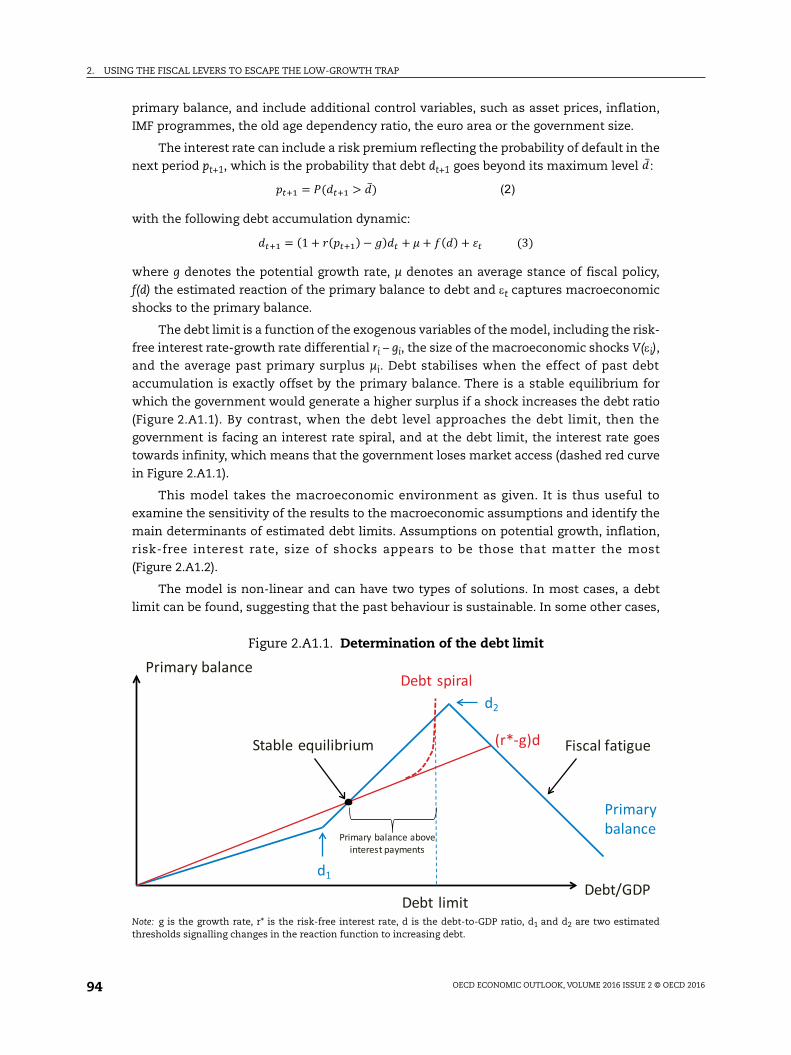
2. USING THE FISCAL LEVERS TO ESCAPE THE LOW-GROWTH TRAP
OECD ECONOMIC OUTLOOK, VOLUME 2016 ISSUE 2 © OECD 201694
primary balance, and include additional control variables, such as asset prices, inflation,
IMF programmes, the old age dependency ratio, the euro area or the government size.
The interest rate can include a risk premium reflecting the probability of default in the
next period pt+1, which is the probability that debt dt+1 goes beyond its maximum level :
with the following debt accumulation dynamic:
where g denotes the potential growth rate, µ denotes an average stance of fiscal policy,
f(d) the estimated reaction of the primary balance to debt and t captures macroeconomic
shocks to the primary balance.
The debt limit is a function of the exogenous variables of the model, including the risk-
free interest rate-growth rate differential ri – gi, the size of the macroeconomic shocks V(i),
and the average past primary surplus µi. Debt stabilises when the effect of past debt
accumulation is exactly offset by the primary balance. There is a stable equilibrium for
which the government would generate a higher surplus if a shock increases the debt ratio
(Figure 2.A1.1). By contrast, when the debt level approaches the debt limit, then the
government is facing an interest rate spiral, and at the debt limit, the interest rate goes
towards infinity, which means that the government loses market access (dashed red curve
in Figure 2.A1.1).
This model takes the macroeconomic environment as given. It is thus useful to
examine the sensitivity of the results to the macroeconomic assumptions and identify the
main determinants of estimated debt limits. Assumptions on potential growth, inflation,
risk-free interest rate, size of shocks appears to be those that matter the most
(Figure 2.A1.2).
The model is non-linear and can have two types of solutions. In most cases, a debt
limit can be found, suggesting that the past behaviour is sustainable. In some other cases,
Figure 2.A1.1. Determination of the debt limit
Note: g is the growth rate, r* is the risk-free interest rate, d is the debt-to-GDP ratio, d1 and d2 are two estimatedthresholds signalling changes in the reaction function to increasing debt.
(2)
= (1 + ( ) ) + + ( ) + (3)
Debt/GDP
Primary balance
(r*-g)d
Debt limit
Fiscal fatigue
Debt spiral Primary balance
Stable equilibrium
Primary balance above interest payments
d1
d2
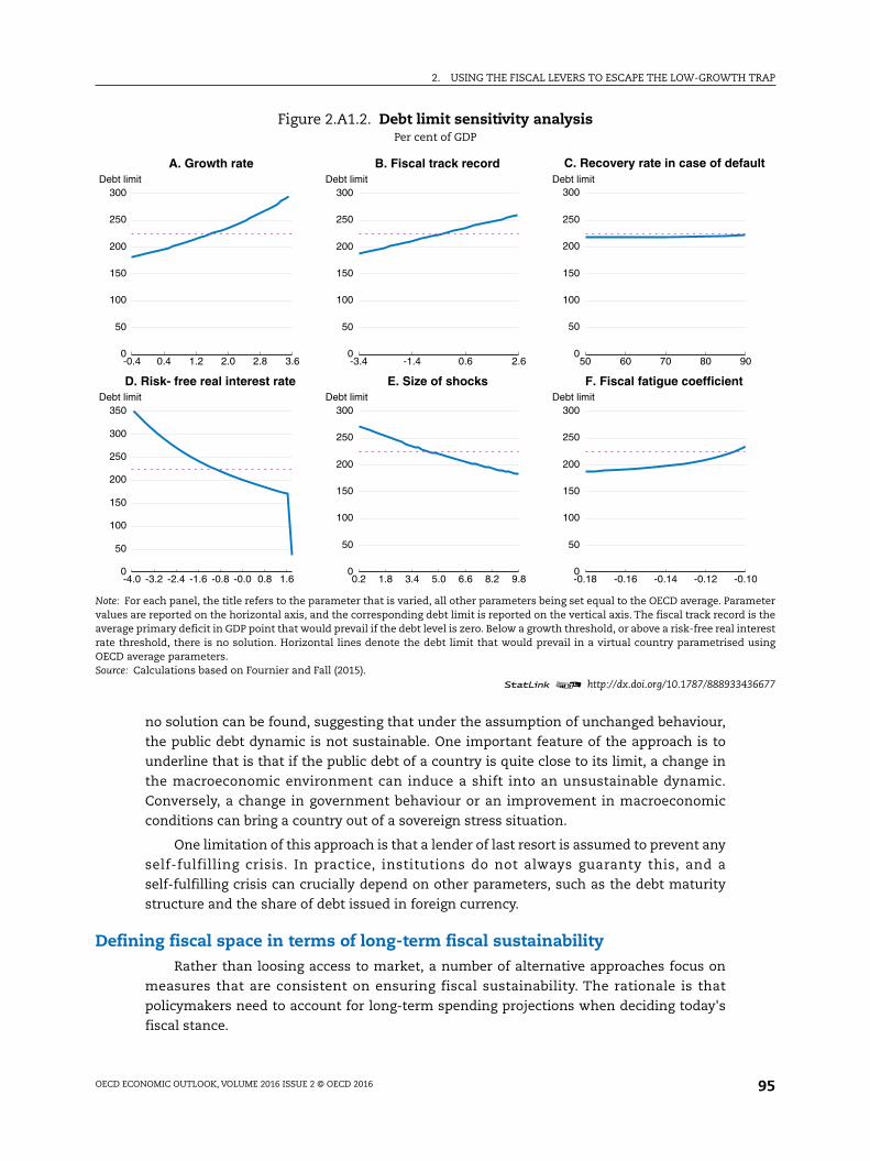
2. USING THE FISCAL LEVERS TO ESCAPE THE LOW-GROWTH TRAP
OECD ECONOMIC OUTLOOK, VOLUME 2016 ISSUE 2 © OECD 2016 95
no solution can be found, suggesting that under the assumption of unchanged behaviour,
the public debt dynamic is not sustainable. One important feature of the approach is to
underline that is that if the public debt of a country is quite close to its limit, a change in
the macroeconomic environment can induce a shift into an unsustainable dynamic.
Conversely, a change in government behaviour or an improvement in macroeconomic
conditions can bring a country out of a sovereign stress situation.
One limitation of this approach is that a lender of last resort is assumed to prevent any
self-fulfilling crisis. In practice, institutions do not always guaranty this, and a
self-fulfilling crisis can crucially depend on other parameters, such as the debt maturity
structure and the share of debt issued in foreign currency.
Defining fiscal space in terms of long-term fiscal sustainabilityRather than loosing access to market, a number of alternative approaches focus on
measures that are consistent on ensuring fiscal sustainability. The rationale is that
policymakers need to account for long-term spending projections when deciding today's
fiscal stance.
Figure 2.A1.2. Debt limit sensitivity analysisPer cent of GDP
Note: For each panel, the title refers to the parameter that is varied, all other parameters being set equal to the OECD average. Parametervalues are reported on the horizontal axis, and the corresponding debt limit is reported on the vertical axis. The fiscal track record is theaverage primary deficit in GDP point that would prevail if the debt level is zero. Below a growth threshold, or above a risk-free real interestrate threshold, there is no solution. Horizontal lines denote the debt limit that would prevail in a virtual country parametrised usingOECD average parameters.Source: Calculations based on Fournier and Fall (2015).
1 2 http://dx.doi.org/10.1787/888933436677
-0.4 0.4 1.2 2.0 2.8 3.60
50
100
150
200
250
300Debt limit
A. Growth rate
-3.4 -1.4 0.6 2.60
50
100
150
200
250
300Debt limit
B. Fiscal track record
50 60 70 80 900
50
100
150
200
250
300Debt limit
C. Recovery rate in case of default
-4.0 -3.2 -2.4 -1.6 -0.8 -0.0 0.8 1.60
50
100
150
200
250
300
350Debt limit
D. Risk- free real interest rate
0.2 1.8 3.4 5.0 6.6 8.2 9.80
50
100
150
200
250
300Debt limit
E. Size of shocks
-0.18 -0.16 -0.14 -0.12 -0.100
50
100
150
200
250
300Debt limit
F. Fiscal fatigue coefficient
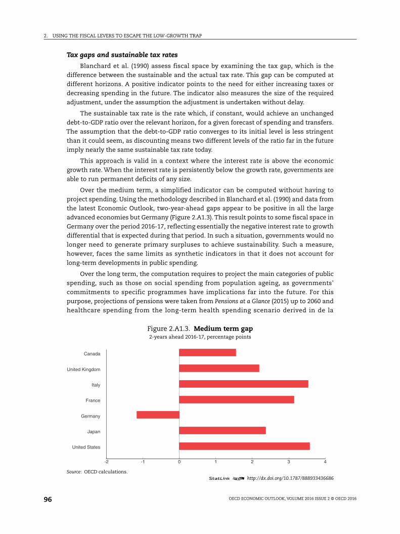
2. USING THE FISCAL LEVERS TO ESCAPE THE LOW-GROWTH TRAP
OECD ECONOMIC OUTLOOK, VOLUME 2016 ISSUE 2 © OECD 201696
Tax gaps and sustainable tax rates
Blanchard et al. (1990) assess fiscal space by examining the tax gap, which is the
difference between the sustainable and the actual tax rate. This gap can be computed at
different horizons. A positive indicator points to the need for either increasing taxes or
decreasing spending in the future. The indicator also measures the size of the required
adjustment, under the assumption the adjustment is undertaken without delay.
The sustainable tax rate is the rate which, if constant, would achieve an unchanged
debt-to-GDP ratio over the relevant horizon, for a given forecast of spending and transfers.
The assumption that the debt-to-GDP ratio converges to its initial level is less stringent
than it could seem, as discounting means two different levels of the ratio far in the future
imply nearly the same sustainable tax rate today.
This approach is valid in a context where the interest rate is above the economic
growth rate. When the interest rate is persistently below the growth rate, governments are
able to run permanent deficits of any size.
Over the medium term, a simplified indicator can be computed without having to
project spending. Using the methodology described in Blanchard et al. (1990) and data from
the latest Economic Outlook, two-year-ahead gaps appear to be positive in all the large
advanced economies but Germany (Figure 2.A1.3). This result points to some fiscal space in
Germany over the period 2016-17, reflecting essentially the negative interest rate to growth
differential that is expected during that period. In such a situation, governments would no
longer need to generate primary surpluses to achieve sustainability. Such a measure,
however, faces the same limits as synthetic indicators in that it does not account for
long-term developments in public spending.
Over the long term, the computation requires to project the main categories of public
spending, such as those on social spending from population ageing, as governments'
commitments to specific programmes have implications far into the future. For this
purpose, projections of pensions were taken from Pensions at a Glance (2015) up to 2060 and
healthcare spending from the long-term health spending scenario derived in de la
Figure 2.A1.3. Medium term gap2-years ahead 2016-17, percentage points
Source: OECD calculations.1 2 http://dx.doi.org/10.1787/888933436686
-2 -1 0 1 2 3 4
Canada
United Kingdom
Italy
France
Germany
Japan
United States
2. USING THE FISCAL LEVERS TO ESCAPE THE LOW-GROWTH TRAP
OECD ECONOMIC OUTLOOK, VOLUME 2016 ISSUE 2 © OECD 2016 97
Maisonneuve and Oliveira Martins (2015). One caveat of using these two sets of projections
is that they may rely, at least over the medium term, on different growth and price
projections. Other spending is assumed to remain constant at 2015 levels.
In this chapter, the calculation is somewhat different from the original computation
done in Blanchard et al. (1990). In particular, tax gaps are derived using the FM, a small
macroeconomic model (see Annex 2.A2 for a brief description). Health spending is partly
considered as an investment and fosters output growth. The sign of the gaps depends to a
very large extent on the assumptions used to project health care spending, which are
traditionally surrounded by large uncertainties, given the difficulty to estimate how
technology affects costs. Measures taken to contain costs in the health sector are found to
increase fiscal limits in all the countries considered. In the same vein, reforms that will
restrain increase in pension spending will also increase fiscal space.
This method presents several advantages. It takes into account future developments
of the economy and long-term spending projections. It is also tractable and relatively easy
to communicate. Gaps can also be computed under a range of policy assumptions.
However, in the current context of persistent low and negative interest rates, this approach
loses some of its relevance. Finally, a major drawback is its reliance on specific
assumptions, such as long-term spending on health care, which are surrounded by large
uncertainties.
Making use of the Laffer curve and defining forward looking debt limits
Bi (2011) and Bi and Leeper (2013) also emphasise long-term sustainability in their
assessment of fiscal limits, a measurement of the government's ability to service its debt.
Empirically those limits are derived from a DSGE framework.The fiscal limit is forward-looking
and depends on expected future policies and how credible those policies are, private
behaviour (consumption-saving and labour-leisure choices) and the fundamental shocks to
the economy.
In this approach, the fiscal limit arises endogenously from the economy's dynamic
Laffer curve, whose shape depends on the state of the economy. The maximum debt level
depends on the expected present value of future maximum primary surpluses. This is
derived from driving tax revenues to the peak of the Laffer curve and driving expenditure
and transfers to some expected levels.
More specifically, a closed economy with linear production technology is considered.
Output depends on the level of productivity and labour supply. Household consumption
and government purchases satisfy the aggregate resource constraint. The gap between
productivity and its steady state follows an autoregressive process of order 1.
At time t, the government may partially default on its liability. The government
finances lump-sum transfers to households and unproductive purchases by collecting tax
revenue through a tax on labour income and issuing one-period bonds. Lump-sum
transfers are countercyclical and government purchases follow an autoregressive process
of order 1. Following Schmitt-Grohe and Uribe (2007), the government increases tax rates
when public debt rises. An increase in the tax rate may or may not increase the tax
revenue, depending on where that actual tax rate is in the Laffer curve. For a given state,
the government can reach the maximum fiscal surplus at the peak of the Laffer curve. At
each point in time and for each state of the economy, the maximum primary balance will
be derived from the difference between these maximum revenues and projected spending
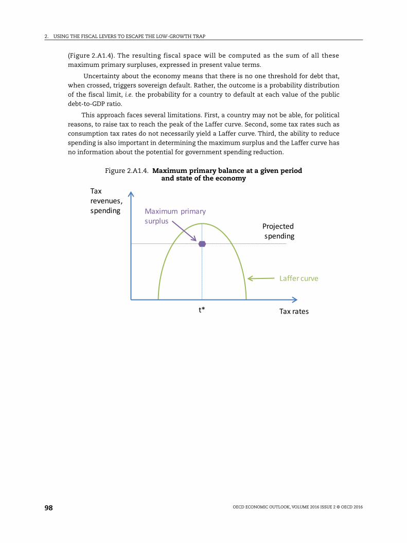
2. USING THE FISCAL LEVERS TO ESCAPE THE LOW-GROWTH TRAP
OECD ECONOMIC OUTLOOK, VOLUME 2016 ISSUE 2 © OECD 201698
(Figure 2.A1.4). The resulting fiscal space will be computed as the sum of all these
maximum primary surpluses, expressed in present value terms.
Uncertainty about the economy means that there is no one threshold for debt that,
when crossed, triggers sovereign default. Rather, the outcome is a probability distribution
of the fiscal limit, i.e. the probability for a country to default at each value of the public
debt-to-GDP ratio.
This approach faces several limitations. First, a country may not be able, for political
reasons, to raise tax to reach the peak of the Laffer curve. Second, some tax rates such as
consumption tax rates do not necessarily yield a Laffer curve. Third, the ability to reduce
spending is also important in determining the maximum surplus and the Laffer curve has
no information about the potential for government spending reduction.
Figure 2.A1.4. Maximum primary balance at a given periodand state of the economy
Laffer curve
t* Tax rates
Tax revenues, spending
Projected spending
Maximum primary surplus

2. USING THE FISCAL LEVERS TO ESCAPE THE LOW-GROWTH TRAP
OECD ECONOMIC OUTLOOK, VOLUME 2016 ISSUE 2 © OECD 2016 99
ANNEX 2.A2
Brief comparison of the models used in the publicinvestment simulations
The three models employed in the analysis share a number of common features. In
particular, the transmission mechanisms of an increase in public investment to the
economy are very similar. In addition to the short-term boost in demand, such a shock
increases output in the long run when it is permanent. When the shock is temporary, the
long-term impact on output is close to zero in the three models.
The definition of the public sector differs across countries and partly explains
observed differences in government investment across countries. One major source of
difference is the extent to which governments subcontract the delivery of public services
to private firms.
Each model has specific features that cast different lights on the examined issues.
● The Fall & Fournier model (F&F) is a long-term stochastic model and allows examining
the impact of uncertainties on simulation outcomes. Twenty-six OECD economies are
modelled. The efficiency of investment is estimated to be a decreasing function of the
initial capital stock level (Fournier, 2016). In addition, interest rates are assumed to be
more sensitive to public debt levels in the euro area countries than in the other OECD
countries.
● The Fiscal Maquette (FM model) encompasses structural features (such as hysteresis)
and some international dimensions, through trade volumes linkages. Only the large
advanced economies and the rest of the world are modelled. As in the F&F model, a rise
in public debt increases the credit risks premium faced by governments.
● NiGEM is a full-fledged international model maintained by the UK National Institute of
Economic and Social Research. All economies, including large emerging-market economies,
are modelled. Individual country models are linked through trade (via world demand
and price competiveness). The model also encompasses a number of options in terms of
monetary policy or fiscal rules and can be run in backward and forward-looking modes.
A more detailed description of the first two models is provided in Mourougane et al.
(2016). More information on the NiGEM model can be found in Barrell et al. (2012).


From:OECD Economic Outlook, Volume 2016 Issue 2
Access the complete publication at:http://dx.doi.org/10.1787/eco_outlook-v2016-2-en
Please cite this chapter as:
OECD (2016), “Using the fiscal levers to escape the low-growth trap”, in OECD Economic Outlook, Volume2016 Issue 2, OECD Publishing, Paris.
DOI: http://dx.doi.org/10.1787/eco_outlook-v2016-2-3-en
This work is published under the responsibility of the Secretary-General of the OECD. The opinions expressed and argumentsemployed herein do not necessarily reflect the official views of OECD member countries.
This document and any map included herein are without prejudice to the status of or sovereignty over any territory, to thedelimitation of international frontiers and boundaries and to the name of any territory, city or area.
You can copy, download or print OECD content for your own use, and you can include excerpts from OECD publications,databases and multimedia products in your own documents, presentations, blogs, websites and teaching materials, providedthat suitable acknowledgment of OECD as source and copyright owner is given. All requests for public or commercial use andtranslation rights should be submitted to [email protected]. Requests for permission to photocopy portions of this material forpublic or commercial use shall be addressed directly to the Copyright Clearance Center (CCC) at [email protected] or theCentre français d’exploitation du droit de copie (CFC) at [email protected].