chapter 2: boundary-value problems in electrostatics: ithschang/notes/ed02.pdf · chapter 2:...

CHAPTER 2: Boundary-Value Problems in Electrostatics: I

Applications of Green’s theorem

1

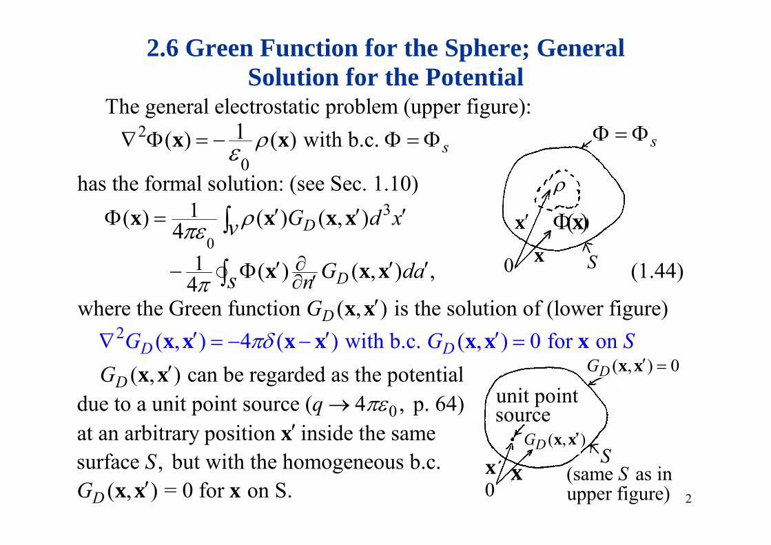
2.6 Green Function for the Sphere; General Solution for the Potential

s 2 The general electrostatic problem (upper figure): ( ) ( ) with b.c. 1

s x x s

3

0

1

( ) ( )

has the formal solution: (see Sec. 1.10)( ) ( ) ( )

s

G d

xx S

( ) x

00

31

1

( ) ( ) ( , )

( ) (

4 DG d x

G

v

x x x x

x x ) (1 44)da x

( )x

( ) (4 Dn G x x

2

, ) , (1.44)

where the Green function ( , ) is the solution( ) 4 ( ) i h

of (lower figure) b ( ) 0 f

D

da

GG G S

s

x

x x

unit point

( , ) 0DG x x

2 ( , ) 4 ( ) with ( , ) can be re

b.c. ( , ) 0 for ong

D D

DGG G S

x x x x

xx x

xx

arded as the potentiald i i ( 4 64)

( , )DG x x

unit pointsource

S

0due to a unit point source ( 4 , p. 64)at an arbitrary position inside the same

f b t ith th h b

q

S

x

x xS

(same as inupper figure)

S0 2

surface , but with the homogeneous b.c. ( , ) = 0 for on S.D

SG x x x

Use (1 44) to find due to a point charge at:Exampl qe 1 x b

2.6 Green Function for the Sphere… (continued)

2

Use (1.44) to find due to a point charge at in infinite space.

( ) ( ) ith b ( ) 0

:Exampl qe 1

q

x b

b2

0 ( ) ( ) with b.c. ( ) 0

In order to use (1.44), we firs

q x x b

t obtain the Green function from( )2 ( , ) 4 ( ) with ( , ) 0 for on S (2)

1D DG G

x x x x x x x

The solution of (2) is 1( , )

Sub ( ) for ( ) and 1/ | | for ( )|

i|D

Dq G

G

x xx x

x b x x x x x nto (1 44) Sub. ( ) for ( ) and 1/ | | for ( , ) iDq G x b x x x x x

03

1| |( )

nto (1.44)

( )1 1 Dq

G

x xx bx x

3

0

( , )1 1( ) ( ) ( , ) ( )4 4

1

DD

GG d x dan

q

v s

x xx x x x x

0

1 4 | |

q

x b

3

2 : ( ) 0 with b.c. ( ) ( , , ) 2 r a aExample x2.6 Green Function for the Sphere… (continued)

Find ( ) in the region (see left figure). First, find ( , ) fromD

r aG

xx x x

2the equation (see right figure)

( , ) 4 (

D

DG x x x ) x

xnS a

xnS a( , ) (D )

with ( , ) 0 on .: points outward from the volume of interest

DG SNote

x xn

( , ) 0DG x x( , , )a

: points outward from the volume of interest. This equation has the solution (see Sec. 2.

12):

a

Note n

2 ( ) 4 ( )G x x x x22

1( , )|

1 1

|D ax

ax

G

xx

xx x x

( , ) 4 ( )in region of interest ( )

DGr a

x x x x

221 22 2

1 1 2 cos xxx x xx

2

1 22 (3)

2 cosa xx 2

: ( , ) ( , ) D D

a

Note G G x x x x angle between x and x’4

2.6 Green Function for the Sphere… (continued)

2 2( ) ( ) ( )G G 2 2

2 2 3 2( , ) ( , ) ( )

' ( 2 cos )D D

x a x a

G G x an x a x a ax

x x x x

3

0 Sub. (3) into (1.44)

( , )1 1( ) ( ) ( ) ( ) DGG d x da

x xx x x x x

0

2 2

( ) ( ) ( , ) ( ) 4 41 ( )( ) (2 19)

DG d x dan

a x aa d

v s

x x x x x

2 2 3 2 ( , , ) (2.19)4 ( 2 cos )

:

a dx a a

Ques nx

tio ss

1. In (3), we h 2 21

| |

2 1

ave ( , ) as a solution of

( ) 4 ( ) But ( ) apparently also

D xaG a x

G G

/x x x xx x

x x x x x x 1| | ( , ) 4 ( ). But ( , ) apparently also

satisfies the same equation. Does this violate the uniqueness thm.?2 C th l

D DG G x xx x x x x x

2ti f ( ) 4 ( ) b itt i thG 2. Can the solu 2tion of ( , ) 4 ( ) be written in the form ( , ) ( )? why?

D

D D

GG G

x x x xx x x x 5

2.1 Method of Images

The method of images is not a general method. It works for someproblems with a simple geometry Consider a point charge locatedqproblems with a simple geometry. Consider a point charge located in front of an infinite and grounded plane conductor (see figure)

q. The

region of interest is 0 and is governed by the Poisson equation:x 0 0 s s

x x qq q

imagecharge2

0

g g y q

( ) ( )q x x y

0s 0s

region ofregion ofx

y y

xy

qq q

00

subject to the boundary condition

region ofinterest

region of interest ( 0) 0.

In order to maintain a zero potential on the cx

onductor, surfaceh ill b i d d (b ) h d W i lcharge will be induced (by ) on the conductor. We may simulate

the effects of the surface charge with a hypothetical "image charge", located symmetrically behind the conductor T

q

q hen 6, located symmetrically behind the conductor. Tq hen, 6

2.1 Method of Images (continued)

1 1 q 0 0

s sx x qq q

imagecharge0

1 14 | | | |

( )

and, by symmetry, ( ) satisfies

q

x y x yx

x

0s 0s

region ofregion ofx

y y

xy

qq q

00

and, by symmetry, ( ) satisfies the boundary condition ( 0) 0.x

x

region ofinterest

region of interest2

2

( ) Operate ( ) with ( ) [ ( ) ( )]q

x

x x y x y (1)0

( ) [ ( ) ( )] x x y x y (1)

In the region of interest ( 0), we have ( ) 0. Thus,( ) obeys the original Poisson equation

x

x yx

20

( ) obeys the original Poisson equation This shows that we must put the image ( ) ( ) ch

q

x

x x y arge outside the region of interest 0 g g

Since ( ) satisfies both the Poisson equation and the boundarycondition in the region of interest, it is a solution. By the uniqueness

x

7

theorem, it is the only solution. Note that the Poisson equation (1) and the solution ( ) are irrelevant outside the region of interest. x

2.2 Point Charge in the Presence of a Grounded Conducting Sphere nConducting Sphere

Refer to the conducting sphere of radius shown in the figure. Assume a point charge

aq

n

Bx

nqg p g

is at ( ). To find for , we put animage charge at ( ). Then,

qr y a r a

q r y a

qay

y q

0 04 4( ) q q

x y x yx

4 42

First set or '=y a ay 0 04 4

B d diti i

q qx y x y

n n n n

First, set , or ,'

so that =

ya y y

yyaa n n n n

0 04 4 Bounday condition requires

( ) 0y aq qa

Note: ' ; hence, ' lies outside the region of interest.'

yy a q

0 04 4( )

y aa ya y

q aq

n n n n

x

'Next, set so that RHS 0. ''Thi i '

q qa y

y a

22

( )ay

y

x y

x yx This gives ' .y aq q q

a y

8

4 4 This is eq i alent to (2 1)q aq

2.2 Point Charge in the Presence of a Grounded Conducting Sphere (continued)

22

0 04 4 This is equivalent to (2.1) Rewrite ( ) and (2.4) of Jackson.ay

q aq

y

x yx y

x

20

In the region of interest ( ), we have ( ) ( ).Thus as in the case of the plane cond

yqr a x x y

uctor satisfies the PoissonThus, as in the case of the plane conductor, satisfies the Poissonequation and the b.c. It is hence the only solution. The -field lines are shown in the figure below.

E

a e s ow t e gu e be ow.

n

Bx

q ynq qa

y

y q

9

: The solution for ( ) can beSurface charge density on the sphere x


: The solution for ( ) can beexpressed in terms of scalars as

1( ) [ ]q

Surface charge density on the sphere

a

x

x

n24 22 2 1/ 2 2 1/ 204 ( )

( 2 cos ) ( 2 cos )where is the angle between and

[ ]q

yya xax y xy y x

x

x .y

B

x

qa ynq

where is the angle between and x . By Gauss's law, the surface chargedensity at point isB

y

y

y

0 02

density at point is

( )r x a

B

E x a x

2

2

4 32 2 3/ 2 2 3/ 28(2 2 cos )2 2 cos

( 2 cos ) ( 2 cos )[ ]yq

aa aa ya aa y ay y a

2

( ) ( 2 cos )yyy y y a

221

(2 5)( )a

q a y 2

22 3/ 2

(2.5)4 (1 2 cos )

( )yy

a aya 10

:Total charge on the sphere


nx

: The total surface charge can be obtainedby integrating over the spherical surface.

Total charge on the sphere

Bqa

y q

nby integrating over the spherical surface.However, it can be deduced from a simpleargument: In the region , the electr a

ricyfield due to the surface charge is exactly

the same as that due to the image charge .b G ' l h l f h b ( )

qa

Hence, by Gauss's law, the total surface charge must be ( ).

:

aq qy Force on q

Since, at the position of charge , the field produced by the imagecharge is the same as that produced by the surface charge, the forceon is the Coulomb force betwen and

qq

q q q

22

on is the Coulomb force betwen and . ( )1 1=

q q qaq qqq y F n

2

2 2

3

1 (2.6)qay n n22

0 04 4( ) ( yay y y

F n 2 22

22 0 (2.6)

4 (1 )) aya

n n

11

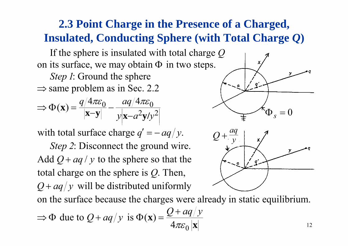
2.3 Point Charge in the Presence of a Charged, Insulated Conducting Sphere (with Total Charge Q)

Insulated, Conducting Sphere (with Total Charge Q)

If the sphere is insulated with total charge on its surface, we may obtain in two steps.

Qon its surface, we may obtain in two steps.

: Ground the sphere same problem as in Sec. 2.2 Step 1

0 0 0

2 24 4( ) q aq

a yy

x y x y/x 0s

with total surface charge . : Disconnect the ground wire.

q aq yStep 2

aqyQ

gAdd / to the sphere so that the total charge on the sphere is . Then,

pQ aq y

Q

will be distributed uniformly on the surface because the Q aq y

charges were already in static equilibrium.

0 due to is ( )

4Q aq yQ aq y

xx 12

Hence, the total is

2.3 Point Charge in the Presence of a Charged, Insulated, Conducting Sphere (continued)

02 2

Hence, the total is 1 ( ) (2.8)

4[ ]

a yq aq Q aq y

y

xx y x y/

x

3

0

0force due toadded charge

4

( / )The force on is the force in (2.6) plus 4

a yyq Q aq yq y

y x y/y

0

0 g

14

qy

F3 2 2

2 2 2(2 ) (2.9)

( )2qa y aQ

yy y y a

y q Q ya

04

2

( )

As , (Coulomb force between point charges)4

yy y y aqQy F

y

04

As , is always attractive even if and have the samey

y a F q Q

sign.

sign.

If there is an excess of electrons on the surface, why don't they leave the surface due to mutual repulsion?

:Question

don t they leave the surface due to mutual repulsion? (See p. 61 for a discussion on the work function of a metal.)

13

2.7 Conducting Spheres with Hemisphere…(to be discussed in Sec. 3.3)(to be d scussed Sec. 3.3)

2.8 Orthogonal Functions and ExpansionsDefinition of Orthogonal Functions :

Consider a set of real or complex functions ( ) ( 1,2, ) which are square integrable on the interval

nU na b

Definition of Orthogonal Functions :

which are square integrable on the interval .in

a b

b

ner product0 m n

orthogonal, if ( ) ( )

( )'s are n m

n

bU U daU

0,

0, 0

m nm n

0,

orthonormal, if ( ) ( ) 1, n m mn

m nbU U da m n

G i l l d th l t fGeometrical analogue: ex, ey, and ez are an orthonormal set ofunit vectors, i.e. emen = mn. By comparison, the dot product emenis similar to the inner product But the algebraic set U () can beis similar to the inner product . But the algebraic set Un() can beinfinite in number. 14

Linearly Independent Functions :

2.8 Orthogonal Functions and Expansions (continued)

The set of ( ) 's are said to be linearly independent if theonly solution of ( ) 0 (for every in the range of

nUa U

Linearly Independent Functions :

only solution of ( ) 0 (for every in the range of

) is 0 for any . If

n nn

n

a U

a b a n

f f i h l h l li l If a set of functions are orthogonal, they are also linearly

independent. P f

0, unless

: ( ) 0n n

n m n

Proofa U

0, unless

( ) ( ) ( ) ( )n n m n n mn n

b ba a

m n

a U U d a U U d

2

f

( ) 0

0n n

baa U d

for any 0 n na

15

Gram-Schmidt Orthogonalization Procedure:2.8 Orthogonal Functions and Expansions (continued)

Orthogonality is a sufficient, but not necessary, condition forlinear independence, i.e. linearly independent functions do nothave to be orthogonal. However, they can be reconstructed into anorthogonal set by the Gram-Schmidt orthogonalization procedure. Consider two vectors, and ( ), as a simple example.These two vectors are not orthogonal, because ( ) 0, but

x x y

x x y

e e ee e e

are linearly independent because ( ) 0 0. We may form two

x x ya b a b e e e new vectors as linear combinations of the old

1 2 1 2

1 2 2

vectors, and + + , and demand 0. 0 1+ 0 1

x x y x

y

e e e e e e e ee e e e1 2 2

1 2 The new set, ( ) and ( ), are thus orthogonal (as wely

x y e e e e l as linearly independent). The same procedure can be applied to algebraic functions.

16

Completeness of a Set of Functions :2.8 Orthogonal Functions and Expansions (continued)

Expand an arbitrary, square integrable function ( ) in terms ofa finite number ( ) of functions in the orthonormal set ( ), n

fN U

( ) (n nf a U 1

) (2.30)

d d fi th ( )

N

nM

2

and define the mean square error ( ) as

( ) ( ) .N

N

N n n

M

bM f a U d If there exists a finite number N0 such that for N > N0 the mean

M b d ll th bit il ll

1 ( ) ( ) .N n n

nM f a U da

square error MN can be made smaller than any arbitrarily smallpositive quantity by proper choice of an’s, then the set Un( ) issaid to be complete and the series representationsaid to be complete and the series representation

1 ( ) ( ) (2.33)n na U f

1is said to converge in the mean to ( ).

nf

17


R it (2 33) ( ) ( ) (2 33)f U

1 Rewrite (2.33): ( ) ( ) (2.33)

Using the orthonormal property of ( ) 's, we get

n nn

n

f a U

U

* ( ) ( ) n nbaa U f d (2.32)

Ch i (2 32) t d b tit t (2 32) i t (2 33)

*

Change in (2.32) to and substitute (2.32) into (2.33)

( ) ( ) ( ) ( ) (2.34)n nbaf U U f d

1

*

( ) ( ) ( ) ( ) ( )

( ) is arbitrary

n nn

n

af f

f U

( ) ( ) ( ) (2.35)nU n

1

(completeness or closure relation)

nn

Jackson, p. 68: "All orthonormal sets of functions normally occurring in mathematical physics have been proved to be

l " (Thi ill b ill d i S 2 9 ) complete." (This statement will be illustrated in Sec. 2.9.)18

example of complete set of orthogonal functionsFourier Series :2.8 Orthogonal Functions and Expansions (continued)

2 2

p p g ( ) :

( ) nik x

a aExponential representation of f x on the interval x

f x a e

( ) f x

2

( )

2 1; ( )

n

n

nn

ik xn n a

a

a a

f x a e

nk a f x e dx

(4)2a 2 a

x

2; ( )n n aa ak a f x e dx

In (4), ( ) is in general a complex function and, even when ( )is real is in general a complex constant

f x f xis real, is in general a complex constant. In the case ( ) is , we have the

naf x real *

*realty condition:

( ) ( ) ( )n na a

P f f l f f

* *

: ( ) ( ) ( )

n n ni in n n

k ik kx x xProof f x real f x f x

a e a e a e

n n

* (since is linearly independent)n

n n nik x

n na ea

1. Why t: " Questions n o " instead of " 0 to " ? 2. Why 2 instead of ?n n

nk n a k n a

19


2 2 ( ) :a aSinusoidal representation of f x on the interval x

01

2 2

( ) n n nik ik ikn n n

n n

x x xf x a e a a e a e

01

cos cos sin sinn n n n n n n nn

a a k x a k x i a k x a k x

0

1 cos sinn n n n n n

na a a k x i a a k

1

0 2n

x

A

Same as (2.36) and (2.37)

01

2( ) cos sin , (5)2

wheren n n n n

nn

aAf x A k x B k x k

( 0 )

( ) ( )

2 22 2

1 2( ) ( ) cosik ikn nn n n na a

a ax xA a a f x e e dx f x k xdxa a

( 0 )n

2

2cos

2( )

nik ikn n

n n n aa x x

k x

iB i a a f x e e dxa a

2 ( )sin naa

f x k xdx

( 1 )n

22 sin

( )n n n a

i kn

fa ax

2( ) na f

20


Di i : It is often more con enient to e press a ph sicalDiscussion: It is often more convenient to express a physicalquantity (a real number) in the exponential representation than inth i id l t ti b th l ffi i t ( )the sinusoidal representation, because the complex coefficient (an)of an exponential term carries twice the information of the real

ffi i t (A B ) f i id l t F l ifcoefficient (An or Bn) of a sinusoidal term. For example, ifx(t) = Re[aeiωt]

i h di l f i l h i ill h lis the displacement of a simple harmonic oscillator, the complex acontains both the magnitude and phase of the displacement. In thesinusoidal representation, the same quantity will be written

x(t) = Acos(ωt) + Bsin(ωt).Exponential terms are also easier to manipulate (such as

multiplication and differentiation). This point will be furtherdiscussed in Ch. 7.

21

Fourier Transform :2.8 Orthogonal Functions and Expansions (continued)

If the interval becomes infinite ( ), we obtain the Fourier transform (see Jackson p.68).

1

a

1( ) ( ) (2.442

ikxf x A k e dk )

1( ) ( ) (2.45)

2

ikxA k f x e dx

( )

Change to in (2.45) and sub. (2.45) into (2.44)1( ) ( )

ik x x

x x

f x dx f x e dk

( )2

( ) ( )

x x

f x dx f x e dk

( )1 k ( )1 ( ) [completeness relation] (2.47)2

Does ( ) contain any more or any less information:

ik x xe dk x x

A kQuestion 1 Does ( ) contain any more or any less information than ( )? : A kQuestio

fn

x 1

22


Does in ( ) have the same dimension nik xQue a f x a estion 2 :

12

Does in ( ) have the same dimension

as ( ) in ( ) ( ) ?

n nn

ikx

Que a f x a e

A k f x A k e d

sti on 2 :

k2

[assuming is a dimensional quantity.]

Rewri

x

( )1te (2 47): ( ) ik x xe dk x x Rewri ( )te (2.47): ( ) 2

Interchange and

e dk x x

x k( )1 ( ), [orthogonality condition] (2.46)

2

i k k xe dx k k

Let and sub. it into (2.46)1 ( )

ixy

y k k

e dx y ( )2

e dx y

Since ( ) ( ), we may write more generally,1 y y

1 ( ) (6)2

ixye dx y23

There are two useful theorems concerning the Fourier integral:2.8 Orthogonal Functions and Expansions (continued)

2 2

There are two useful theorems concerning the Fourier integral: (1) Parseval's theorem :

The Parseval's theorem states ( ) ( ) (7)

f x dx A k dkThe Parseval s theorem states ( ) ( ) (7)

: f x dx A k dk

Proof 1( ) ( ) (2 44) ikxf x A k e dk Rewrite the Fo

( ) ( ) (2.44)2urier transform:1( ) ( ) (2 45)

ikx

f x A k e dk

A k f x e dx

2 *

( ) ( ) (2.45)2

( ) ( ) ( )

A k f x e dx

f x dx f x f x dx

*

( ) ( ) ( )

1 1 ( ) ( ) 2 2

ikx ik x

f f f

dx A k e dk A k e dk2 2

dk 2* ( )1( ) ( ) ( )2

i k k xA k dk A k dxe A k dk

( )

( ) ( ) ( )2

k k 24


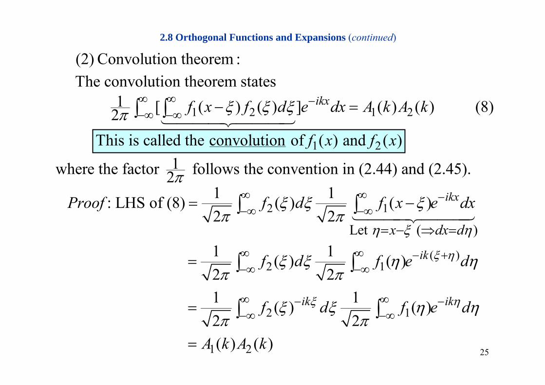
(2) Convolution theorem : (2) Convolution theorem :The convolution theorem states

1 [ ( ) ( ) ] ( ) ( ) (8) ikx

f x f d e dx A k A k1 2 1 2

1

1 [ ( ) ( ) ] ( ) ( ) (8)2 This is called the convolution of ( ) and

f x f d e dx A k A k

f x f2( )x1 21where the factor follows the convention in (2.44) and (2.45).2

1 1

k2 1

Let ( )

1 1 : LHS of (8) ( ) ( )2 2

ikx

x dx d

Proof f d f x e dx

2 1

( )1 1 ( )2 2

f d f ( )( ) ike d

2 11 1 ( ) ( )2 2

ik ikf d f e d

1 2

2 2 ( ) ( )

A k A k

25

2.9 Separation of Variables, Laplace Equation in Rectangular CoordinatesRectangular Coordinates

2 2 22

2 2 2Laplace equation in 0 (2.48)C t i di t

2 2 2 ( )Cartesian coordinates

Let ( , , )= ( ) ( ) ( ) (2.49)x y z

x y z X x Y y Z z

2 2

2 21 1 1d X d YX Ydx dy

2

2 0 (2.50)d ZZ dz

dx dy

Since this equation holds for arbitrary values of , , and , each of the three terms must be separately constant.

dzx y z

22

2

of the three terms must be separately constant.

; d X dXdx

2 2

2 2 2 2 22 2; subject to Y d ZY Z

dy d

dx2 2( ) ; ( ) ; ( ) with

i x i y zzi x i y

dy dz

X x Y y Z ze e eee

zi x i y ee e

26

2.9 Separation of Variables, Laplace Equation in Rectangular Coordinates (continued)

: Find inside a charge-free rectangular box (see figure)Example

( ) i ix xX x Ae Be

: Find inside a charge free rectangular box (see figure) with the b.c. ( , , ) = ( , ) and 0 on other sides.Example

x y z c V x y

z

( ) (0) 0 ( ) 'sin ( ) 0 1 2

i ix x

n

X x Ae BeX B A X A e e A xX a n

z

1

( ) 0 , 1, 2,

( ) sinn

n nn

naX a n

X x A x

y

1

Similarly, ( ) .(0) 0 and ( ) 0 give

ni iy yY y Ae Be

Y Y b

y

1

(0) 0 and ( ) 0 give ( ) sinm m

m

Y Y bY y A y

, m

mb

x Solution for : ( ) (0) 0 ( ) ( ) ''sinh

z z

z zZ Z z Ae Be

Z B A Z z A e e A z

22

, 1sin sin sinh , (2.56)n mnmnm n m nm

n mA x y z

27


To find we apply the b c on the plane:A z c To find , we apply the b.c. on the plane: ( , , ) ( , )

nmA z cx y z c V x y

, 1

( , ) sin sin sinh (2.57)

4

nm n m nmn m

b

V x y A x y c

0 04 (2.58)

sinh( , )sin sinnm

nm

a bn mA

ab cdx dyV x y x y

Q tiQuestions:1. The method of images is not a general method, but the method of

i i th l f ti i Wh ?expansion in orthogonal functions is. Why?2. In electrostatics, only charges can produce Φ. In this problem,

0 h th b Φ ? = 0, how can there be Φ ?3. Can we find the surface charge distribution ( ) on the walls from

h k l d f Φ i id h b ? If d h di i ?the knowledge of Φ inside the box? If so, under what condition?28

:Discussion


1

:

Rewrite (2.57): ( , ) sin sin sinh ,nm n m nmn m

Discussion

V x y A x y c

z

, 1

where and .This is a good example to substantiate

n m

n mmb

na

y

This is a good example to substantiatethe following statement on physics ground:"All orthonormal sets of functions normally

xoccurring in mathematical physics have beenproved to be complete." (p. 68)

( ) i ( ) d i ( ) h l f i In (2.57), sin( ) and sin ( ) are orthogonal functionsgenerated in a physics problem. P

n mx y hysically, we expect the problem

to have a solution for any boundary condition on the surface z cto have a solution for any boundary condition on the surface , i.e. for any function ( , ) specified in (2.57). Thus, sin( ) and and sin ( ) must each form a co

n

m

z cV x y x

y

mplete set in order to represent ( )m y p pan arbitrary ( , ).V x y

29

Homework of Chap. 2

Problems: 1, 2, 3, 4, 5,, , , , ,

9, 23, 26

30

chapter 2: boundary-value problems in electrostatics: ithschang/notes/ed02.pdf · chapter 2:...

Documents