chapter 2: bayesian decision theory (part 2)
TRANSCRIPT
Chapter 2:
Bayesian Decision Theory (Part 2)
Minimum-Error-Rate Classification
Classifiers, Discriminant Functions and Decision Surfaces
The Normal Density
Entropy and Information
All materials used in this course were taken from the textbook “Pattern Classification” by Duda et al., John Wiley & Sons, 2001
with the permission of the authors and the publisher
2
Minimum-Error-Rate Classification
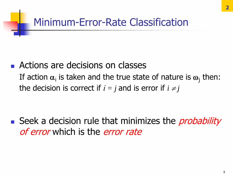
Actions are decisions on classes
If action i is taken and the true state of nature is j then:
the decision is correct if i = j and is error if i j
Seek a decision rule that minimizes the probability of error which is the error rate
3
3
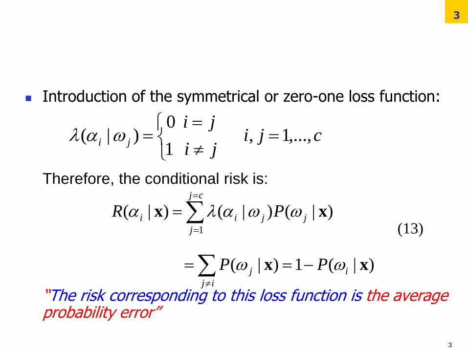
Introduction of the symmetrical or zero-one loss function:
Therefore, the conditional risk is:
“The risk corresponding to this loss function is the average probability error”
cjiji
jiji ,...,1,
1
0)|(
ij
ij
cj
j
jjii
PP
PR
)|(1)|(
)|()|()|(1
xx
xx
3
(13)
4
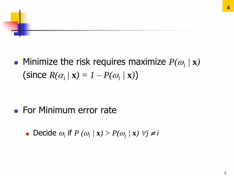
Minimize the risk requires maximize P(i | x)
(since R(i | x) = 1 – P(i | x))
For Minimum error rate
Decide i if P (i | x) > P(j | x) j i
3
5
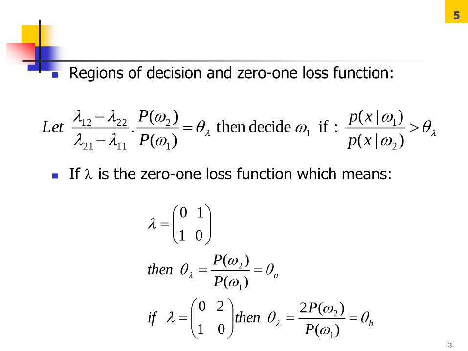
Regions of decision and zero-one loss function:
If is the zero-one loss function which means:
b
a
P
Pthenif
P
Pthen
)(
)(2
0 1
2 0
)(
)(
0 1
1 0
1
2
1
2
)|(
)|( :if decide then
)(
)(.
2
11
1
2
1121
2212
xp
xp
P
PLet
3
6
3
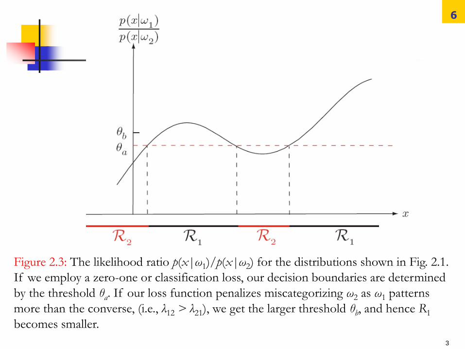
Figure 2.3: The likelihood ratio p(x|ω1)/p(x|ω2) for the distributions shown in Fig. 2.1.
If we employ a zero-one or classification loss, our decision boundaries are determined
by the threshold θa. If our loss function penalizes miscategorizing ω2 as ω1 patterns
more than the converse, (i.e., λ12 > λ21), we get the larger threshold θb, and hence R1
becomes smaller.
7
Minimax Criterion
We may want to design our classifier to perform well over a range of prior probabilities.
A reasonable approach is then to design our classifier so that the worst overall risk for any value of the priors is as small as possible — that is, minimize the maximum possible overall risk.
Let R1 denote that (as yet unknown) region in feature space where the classifier decides ω1 and likewise for R2 and ω2
8
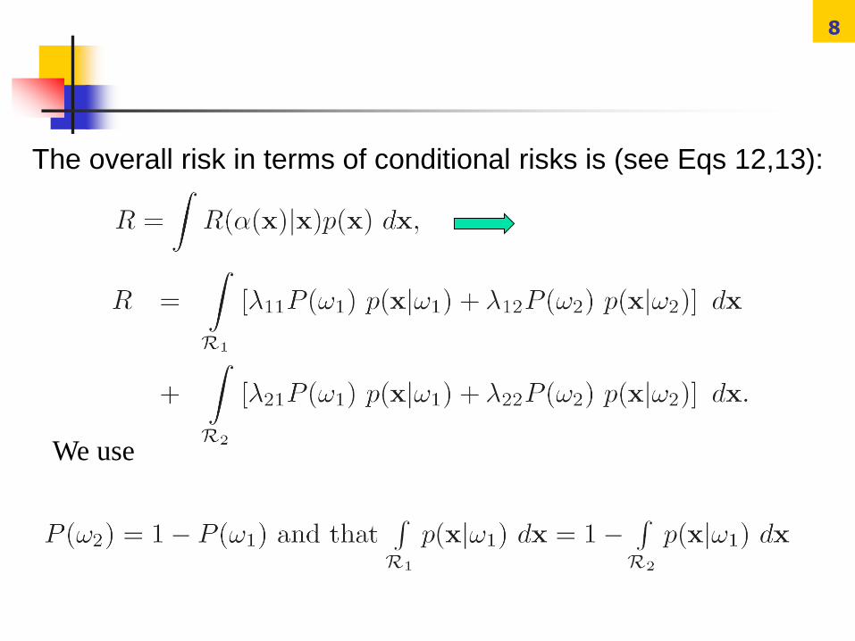
The overall risk in terms of conditional risks is (see Eqs 12,13):
We use
9
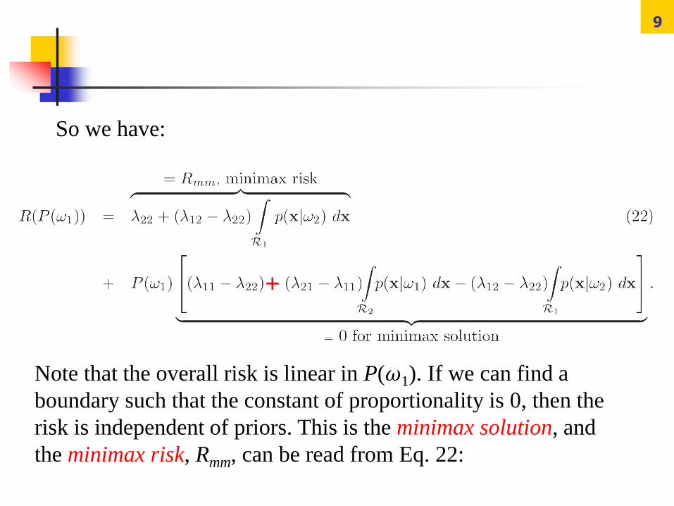
So we have:
Note that the overall risk is linear in P(ω1). If we can find a
boundary such that the constant of proportionality is 0, then the
risk is independent of priors. This is the minimax solution, and
the minimax risk, Rmm, can be read from Eq. 22:
+
10
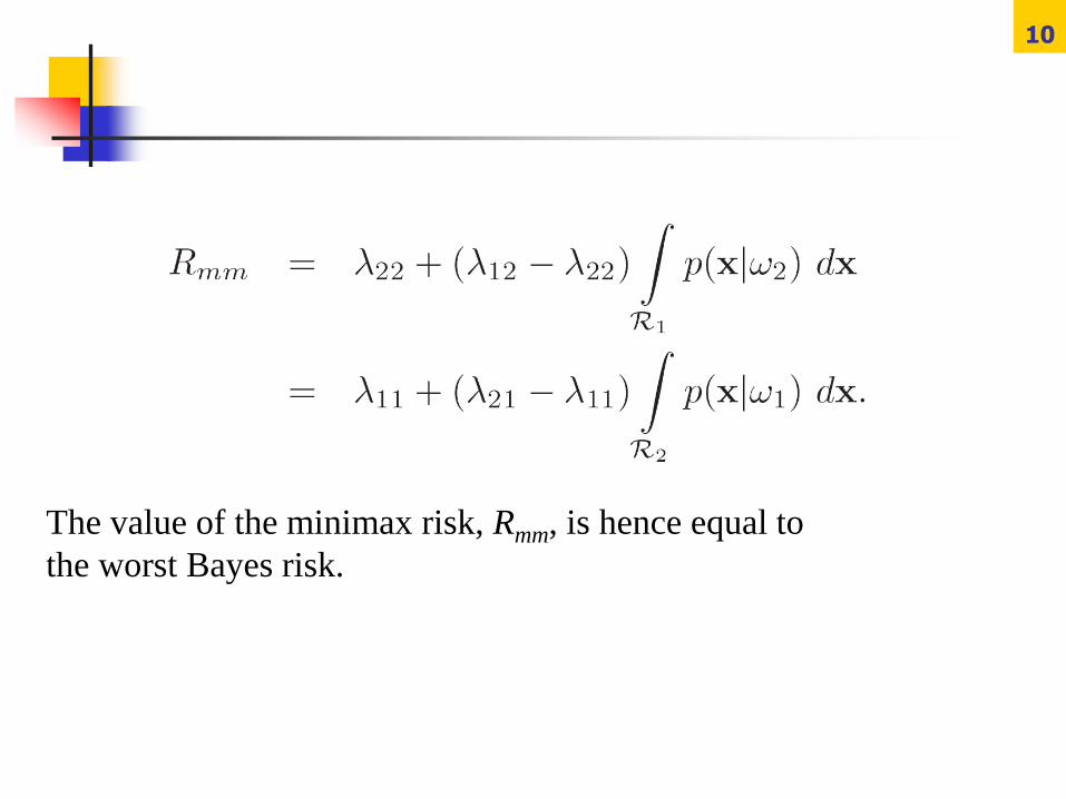
The value of the minimax risk, Rmm, is hence equal to
the worst Bayes risk.
11
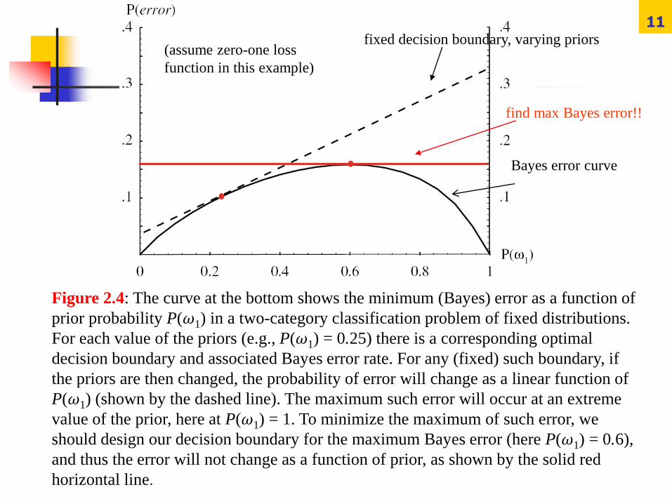
Figure 2.4: The curve at the bottom shows the minimum (Bayes) error as a function of
prior probability P(ω1) in a two-category classification problem of fixed distributions.
For each value of the priors (e.g., P(ω1) = 0.25) there is a corresponding optimal
decision boundary and associated Bayes error rate. For any (fixed) such boundary, if
the priors are then changed, the probability of error will change as a linear function of
P(ω1) (shown by the dashed line). The maximum such error will occur at an extreme
value of the prior, here at P(ω1) = 1. To minimize the maximum of such error, we
should design our decision boundary for the maximum Bayes error (here P(ω1) = 0.6),
and thus the error will not change as a function of prior, as shown by the solid red
horizontal line.
fixed decision boundary, varying priors
find max Bayes error!!
Bayes error curve
(assume zero-one loss
function in this example)
Neyman-Pearson Criterion
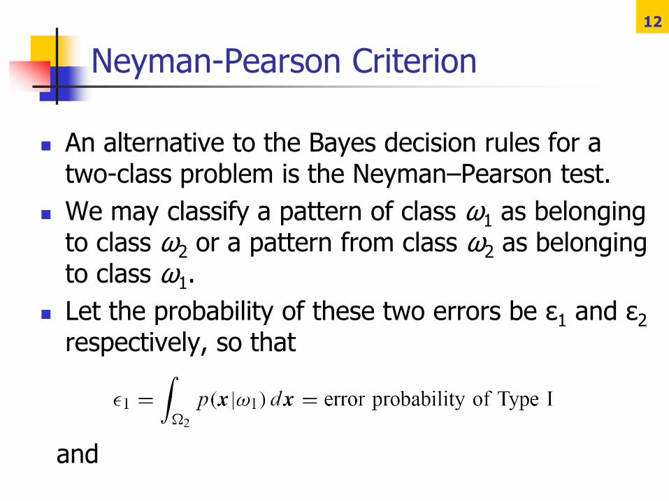
An alternative to the Bayes decision rules for a two-class problem is the Neyman–Pearson test.
We may classify a pattern of class ω1 as belonging to class ω2 or a pattern from class ω2 as belonging to class ω1.
Let the probability of these two errors be ε1 and ε2
respectively, so that
and
12
The Neyman–Pearson decision rule is to minimise the error ε1 subject to ε2 being equal to a constant, ε0, say.
If class ω1 is termed the positive class and class ω2 the negative class, then ε1 is referred to as the false negative rate, the proportion of positive samples incorrectly assigned to the negative class; ε2 is the false positive rate, the proportion of negative samples classifed as positive.
13
14
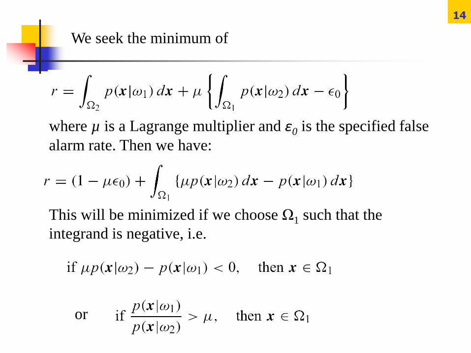
We seek the minimum of
where µ is a Lagrange multiplier and ε0 is the specified false
alarm rate. Then we have:
This will be minimized if we choose Ω1 such that the
integrand is negative, i.e.
or
15
Thus the decision rule depends only on the within-class
distributions and ignores the a priori probabilities.
The threshold µ is chosen so that
the specified false alarm rate. However, in general µ cannot
be determined analytically and requires numerical calculation.
Statistical Pattern Recognition, Third Edition. Andrew R. Webb • Keith D. Copsey
Often, the performance of the decision rule is summarized in a
receiver operating characteristic (ROC) curve, which plots the
true positive against the false positive i.e.1-ε1 vs ε2 as the
threshold μ is varied..
16
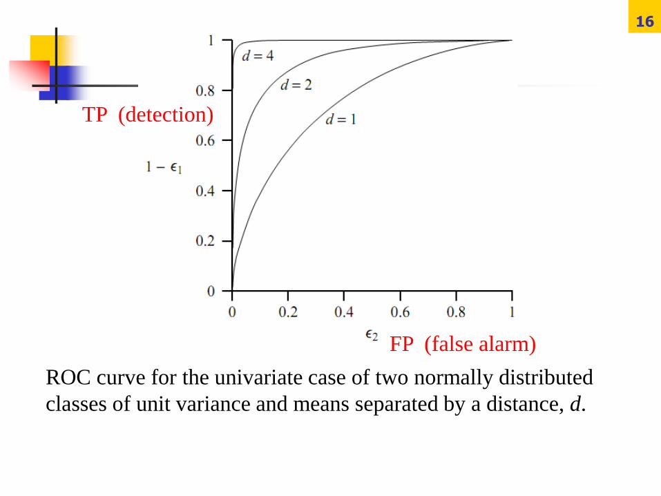
FP (false alarm)
ROC curve for the univariate case of two normally distributed
classes of unit variance and means separated by a distance, d.
TP (detection)
17
Classifiers, Discriminant Functionsand Decision Surfaces
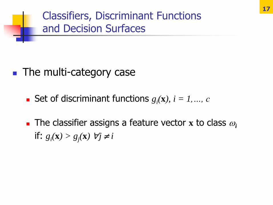
The multi-category case
Set of discriminant functions gi(x), i = 1,…, c
The classifier assigns a feature vector x to class i
if: gi(x) > gj(x) j i
18
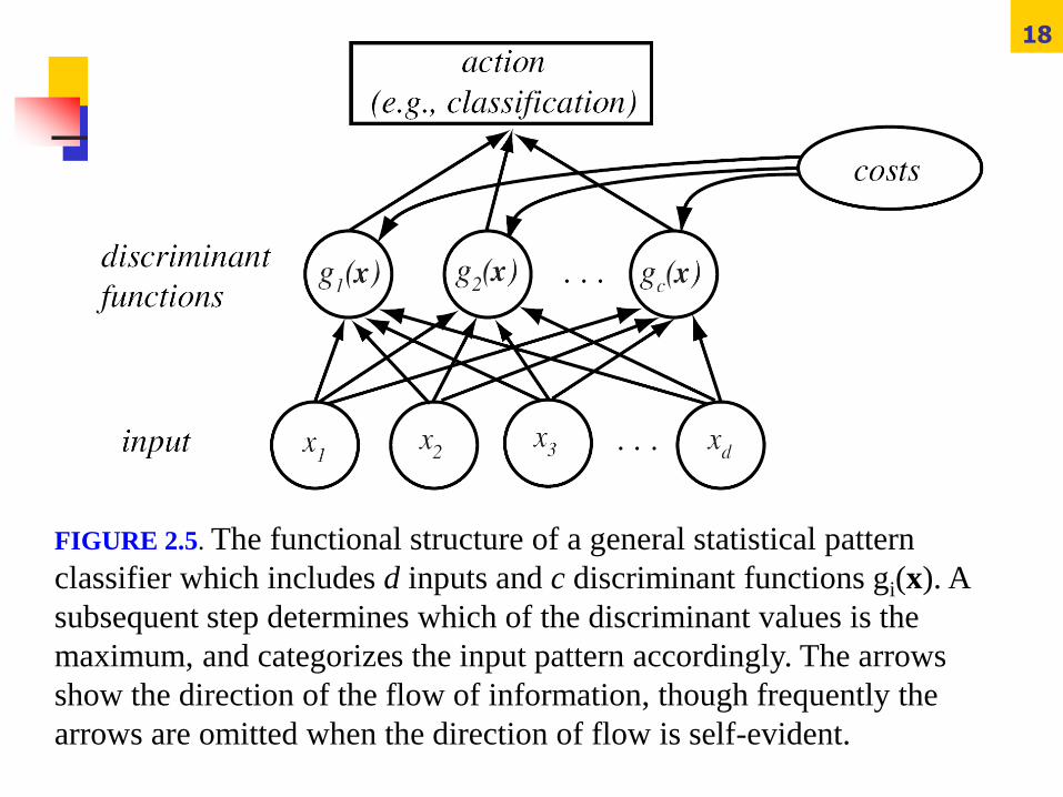
FIGURE 2.5. The functional structure of a general statistical pattern
classifier which includes d inputs and c discriminant functions gi(x). A
subsequent step determines which of the discriminant values is the
maximum, and categorizes the input pattern accordingly. The arrows
show the direction of the flow of information, though frequently the
arrows are omitted when the direction of flow is self-evident.
19
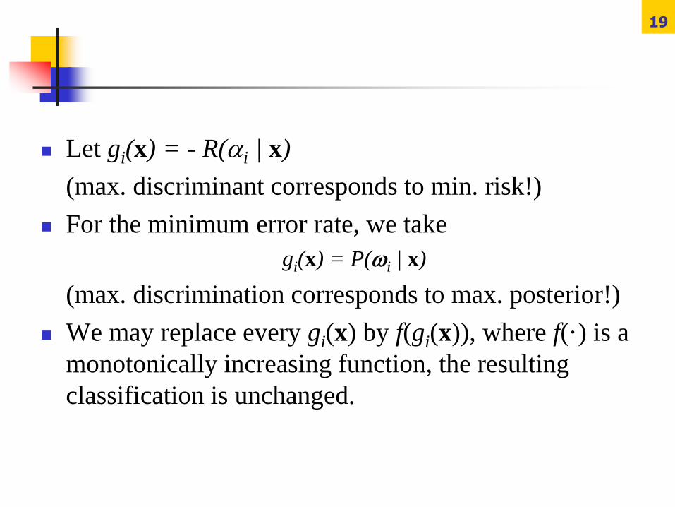
Let gi(x) = - R(i | x)
(max. discriminant corresponds to min. risk!)
For the minimum error rate, we take
gi(x) = P(i | x)
(max. discrimination corresponds to max. posterior!)
We may replace every gi(x) by f(gi(x)), where f(·) is a
monotonically increasing function, the resulting
classification is unchanged.
20
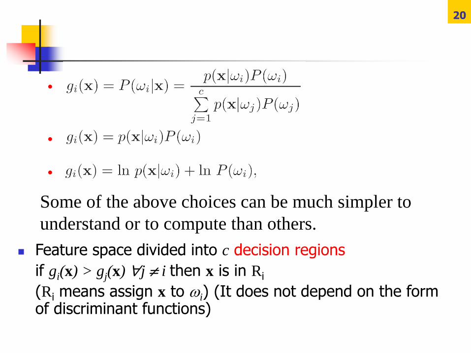
Some of the above choices can be much simpler to
understand or to compute than others.
Feature space divided into c decision regions
if gi(x) > gj(x) j i then x is in Ri
(Ri means assign x to i) (It does not depend on the form of discriminant functions)
•
•
•
21
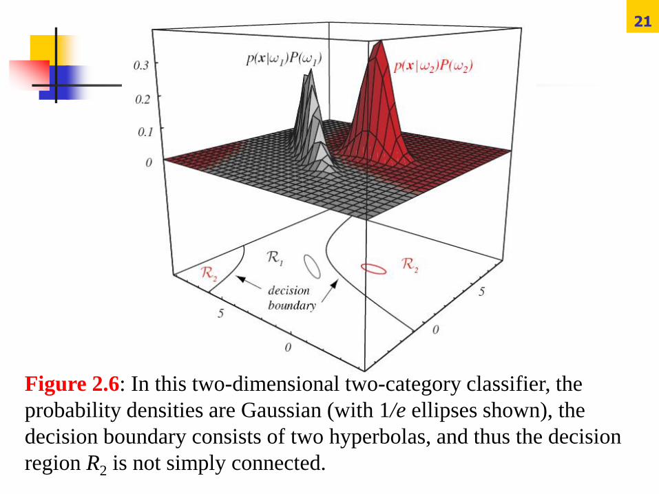
Figure 2.6: In this two-dimensional two-category classifier, the
probability densities are Gaussian (with 1/e ellipses shown), the
decision boundary consists of two hyperbolas, and thus the decision
region R2 is not simply connected.
22
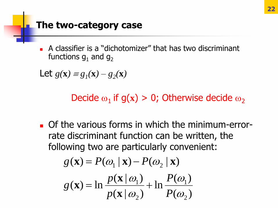
The two-category case
A classifier is a “dichotomizer” that has two discriminant functions g1 and g2
Let g(x) g1(x) – g2(x)
Decide 1 if g(x) > 0; Otherwise decide 2
Of the various forms in which the minimum-error-rate discriminant function can be written, the following two are particularly convenient:
1 2
1 1
2 2
( ) ( | ) ( | )
( | ) ( )( ) ln ln
( | ) ( )
g P P
p Pg
p P
x x x
xx
x
23
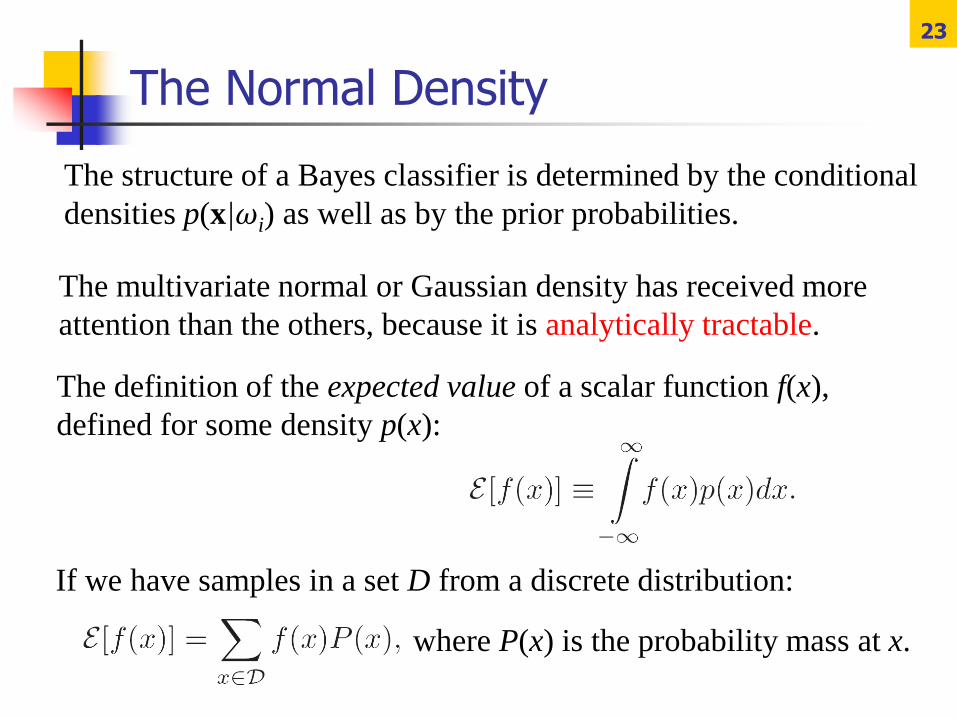
The Normal Density
The structure of a Bayes classifier is determined by the conditional
densities p(x|ωi) as well as by the prior probabilities.
The multivariate normal or Gaussian density has received more
attention than the others, because it is analytically tractable.
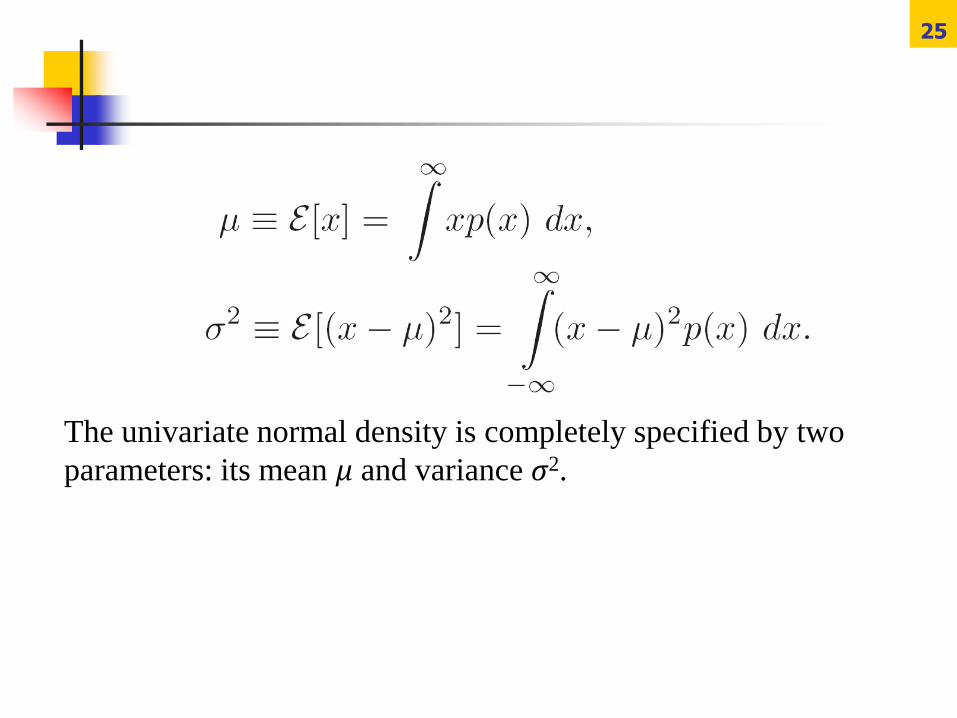
The definition of the expected value of a scalar function f(x),
defined for some density p(x):
If we have samples in a set D from a discrete distribution:
where P(x) is the probability mass at x.
24
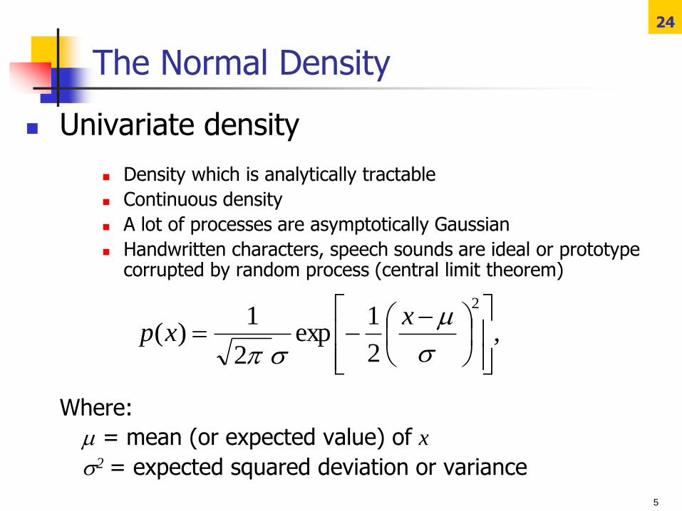
The Normal Density
Univariate density
Density which is analytically tractable
Continuous density
A lot of processes are asymptotically Gaussian
Handwritten characters, speech sounds are ideal or prototype corrupted by random process (central limit theorem)
Where:
= mean (or expected value) of x
2 = expected squared deviation or variance
,2
1exp
2
1)(
2
xxp
5
25
The univariate normal density is completely specified by two
parameters: its mean μ and variance σ2.
26
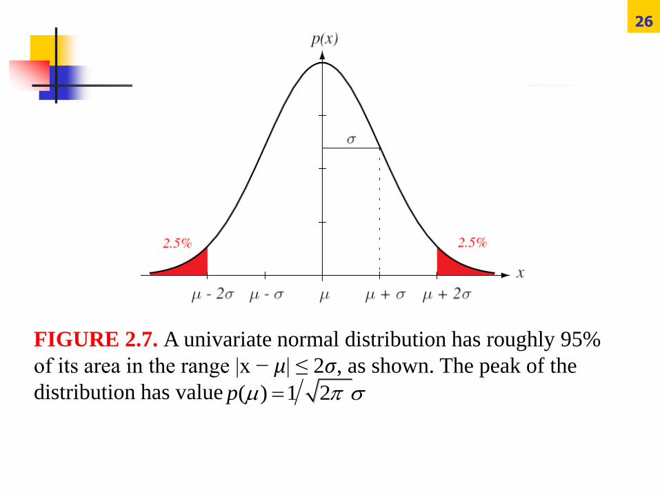
FIGURE 2.7. A univariate normal distribution has roughly 95%
of its area in the range |x − μ| ≤ 2σ, as shown. The peak of the
distribution has value ( ) 1 2 p
27
Entropy and information
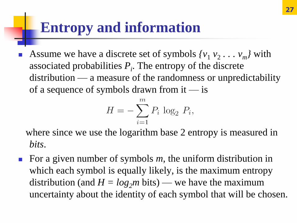
Assume we have a discrete set of symbols {v1 v2 . . . vm} with
associated probabilities Pi. The entropy of the discrete
distribution — a measure of the randomness or unpredictability
of a sequence of symbols drawn from it — is
where since we use the logarithm base 2 entropy is measured in
bits.
For a given number of symbols m, the uniform distribution in
which each symbol is equally likely, is the maximum entropy
distribution (and H = log2m bits) — we have the maximum
uncertainty about the identity of each symbol that will be chosen.
28
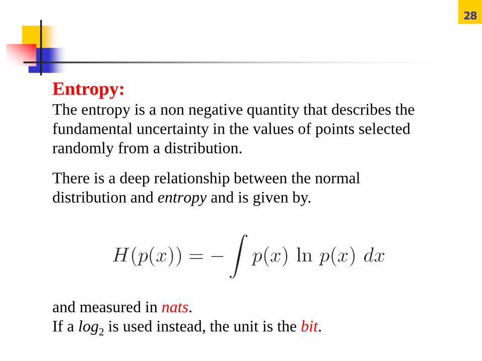
There is a deep relationship between the normal
distribution and entropy and is given by.
and measured in nats.
If a log2 is used instead, the unit is the bit.
Entropy:The entropy is a non negative quantity that describes the
fundamental uncertainty in the values of points selected
randomly from a distribution.
29
It can be shown that the normal distribution has the maximum entropy of all distributions having a given mean and variance.
As stated by the Central Limit Theorem, the aggregate effect of a large number of small, independent random disturbances will lead to a Gaussian distribution.
The Kullback-Leibler Divergence or the relative entropy
30
Consider some unknown distribution p(x), and
suppose that we have modelled this using an
approximating distribution q(x). If we use q(x) to
construct a coding scheme for the purpose of
transmitting values of x to a receiver, then the
average additional amount of information (in nats)
required to specify the value of x (assuming we
choose an efficient coding scheme) as a result of
using q(x) instead of the true distribution p(x) is
given by:From: Theodoridis & Koutroumbas
31
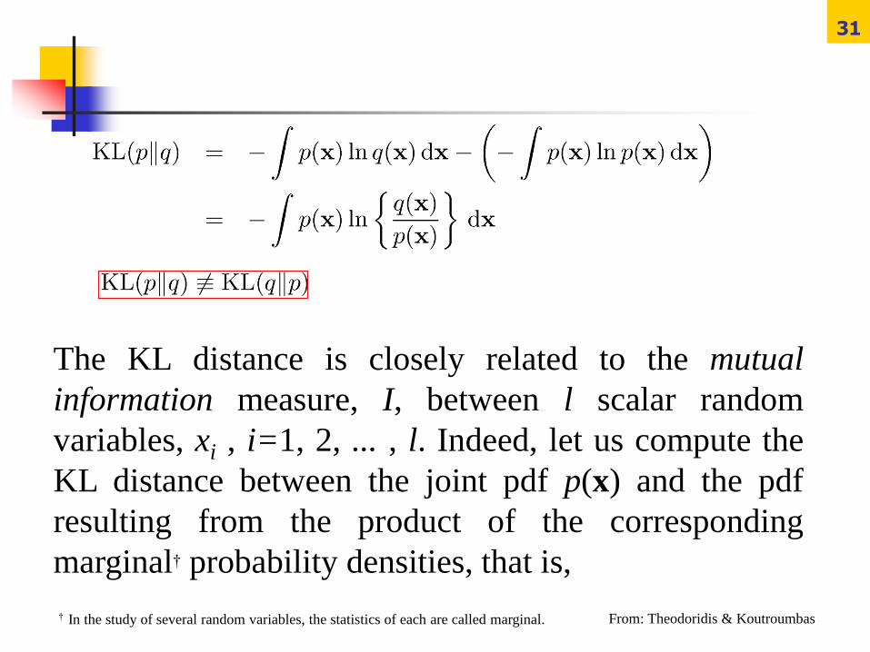
The KL distance is closely related to the mutual
information measure, I, between l scalar random
variables, xi , i=1, 2, ... , l. Indeed, let us compute the
KL distance between the joint pdf p(x) and the pdf
resulting from the product of the corresponding
marginal† probability densities, that is,
From: Theodoridis & Koutroumbas† In the study of several random variables, the statistics of each are called marginal.
32
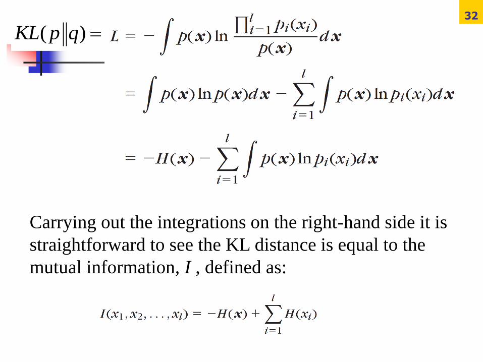
Carrying out the integrations on the right-hand side it is
straightforward to see the KL distance is equal to the
mutual information, I , defined as:
( )KL p q
33
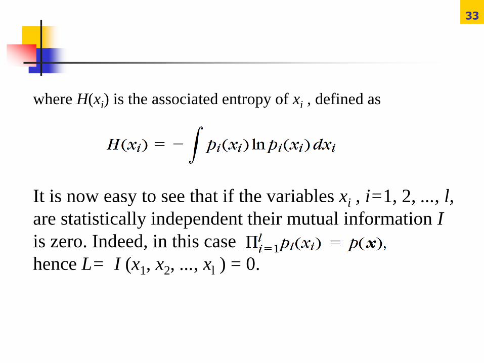
where H(xi) is the associated entropy of xi , defined as
It is now easy to see that if the variables xi , i=1, 2, ..., l,
are statistically independent their mutual information I
is zero. Indeed, in this case
hence L= I (x1, x2, ..., xl ) = 0.
34
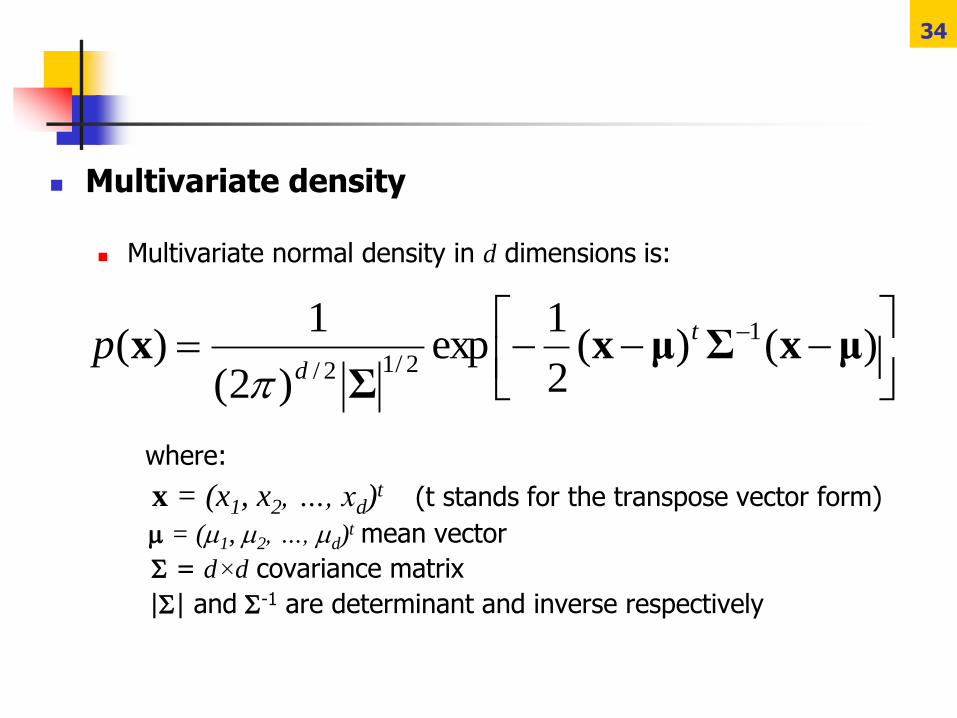
Multivariate density
Multivariate normal density in d dimensions is:
where:
x = (x1, x2, …, xd)t (t stands for the transpose vector form)
= (1, 2, …, d)t mean vector
= d×d covariance matrix
|| and -1 are determinant and inverse respectively
)()(
2
1exp
)2(
1)( 1
2/12/μxΣμx
Σx
t
dp
35
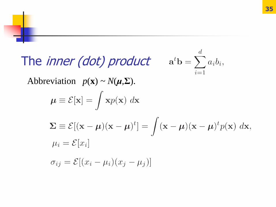
The inner (dot) product
Abbreviation p(x) ~ N(μ,Σ).
36
The covariance matrix Σ is always symmetric and
positive semidefinite.
(A matrix A is pos. semidefinite if: for any z.)
In the case in which Σ is positive definite, the
determinant of Σ is strictly positive.
The diagonal elements σii are the variances of the
respective xi (i.e., σ2i ), and the off-diagonal elements
σij are the covariances of xi and xj .
If xi and xj are statistically independent, σij = 0.
0t z Az
37
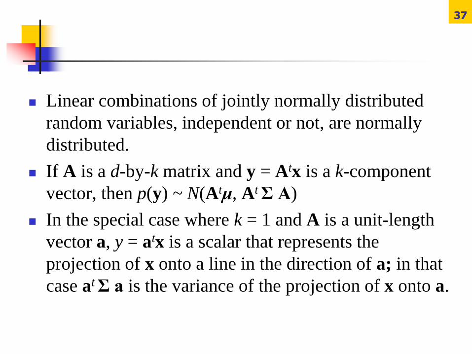
Linear combinations of jointly normally distributed
random variables, independent or not, are normally
distributed.
If A is a d-by-k matrix and y = Atx is a k-component
vector, then p(y) ~ N(Atμ, At Σ A)
In the special case where k = 1 and A is a unit-length
vector a, y = atx is a scalar that represents the
projection of x onto a line in the direction of a; in that
case at Σ a is the variance of the projection of x onto a.
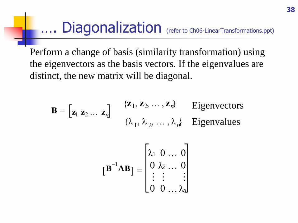
…. Diagonalization (refer to Ch06-LinearTransformations.ppt)
Perform a change of basis (similarity transformation) using
the eigenvectors as the basis vectors. If the eigenvalues are
distinct, the new matrix will be diagonal.
B z1 z2 zn=z1 z2 zn{ , } Eigenvectors
1 2 n{ , } Eigenvalues
n
B1–AB[ ]
1 0 0
0 2 0
0 0
=
38
39
[ ]1
t
t
t -1 t
... matrix consisting of eigenvectors
use as the transformation matrix
covariance matrix of transformed vector
note: ( ) and
n
t
d d d
y x
Φ φ φ
y Φ x Φ A
Φ Φ Λ
Φ Φ Φ Φ
1/2 t 1/2 t
1/2
1/2 t 1/2 1/2 1/2
( )
use as the transformation matrix
covariance matrix of transformed vector is identity matrix
y x
y Λ Φ x ΦΛ x
ΦΛ A
Λ Φ ΦΛ Λ ΛΛ I
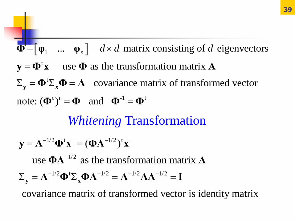
Whitening Transformation
40
If we define Φ to be the matrix whose columns are the
orthonormal eigenvectors of Σ, and Λ the diagonal
matrix of the corresponding eigenvalues, then the
transformation Aw = ΦΛ-1/2 applied to the coordinates
insures that the transformed distribution has covariance
matrix equal to the identity matrix.
In signal processing, the transform Aw is called a
whitening transformation, since it makes the spectrum
of eigenvectors of the transformed distribution uniform.
Properties
41
The multivariate normal density is completely
specified by d + d(d + 1)/2 parameters — the
elements of the mean vector μ and the independent
elements of the covariance matrix Σ.
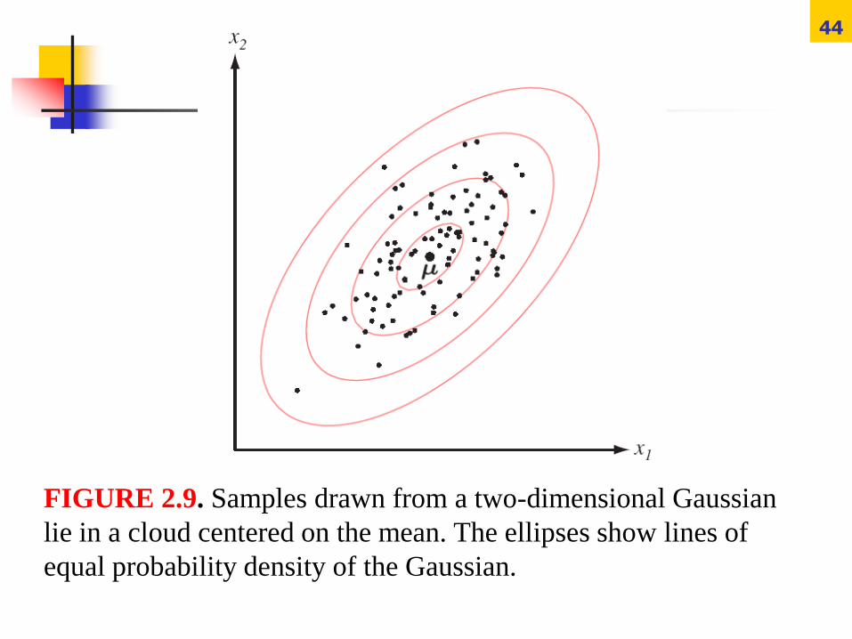
Samples drawn from a normal population tend to fall
in a single cloud or cluster (Fig. 2.9); the center of
the cluster is determined by the mean vector, and the
shape of the cluster is determined by the covariance
matrix.
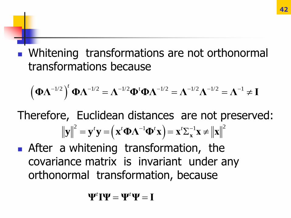
Whitening transformations are not orthonormal transformations because
Therefore, Euclidean distances are not preserved:
After a whitening transformation, the covariance matrix is invariant under any orthonormal transformation, because
42
1/2 1/2 1/2 t 1/2 1/2 1/2 1t
ΦΛ ΦΛ Λ ΦΦΛ Λ Λ Λ I
2 21 1t t t t xy y y xΦΛ Φ x x x x
t t Ψ IΨ Ψ Ψ I
43
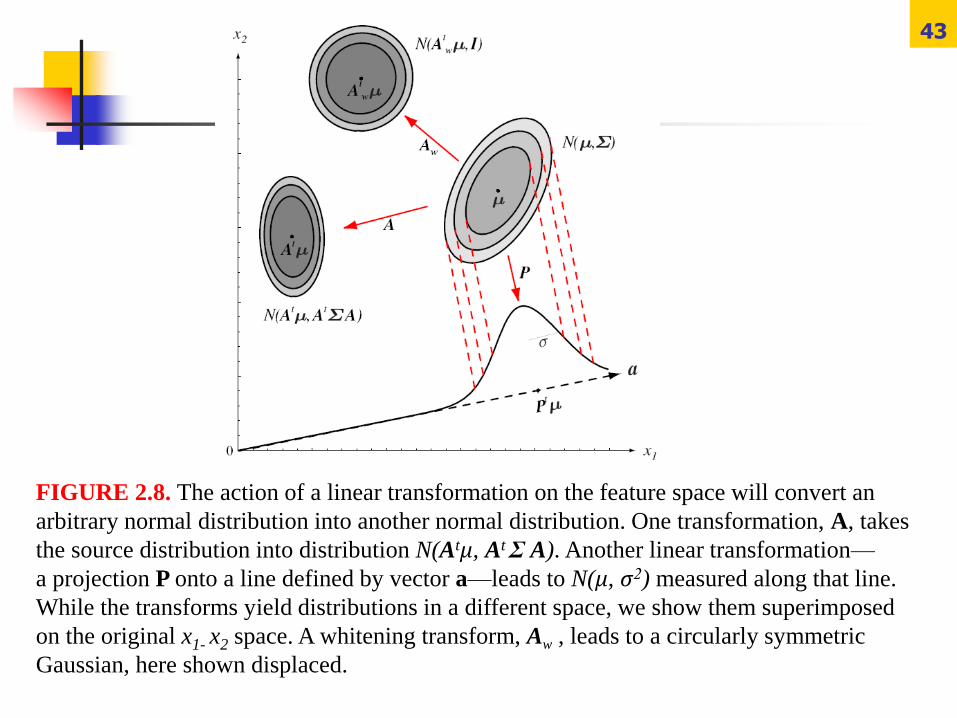
FIGURE 2.8. The action of a linear transformation on the feature space will convert an
arbitrary normal distribution into another normal distribution. One transformation, A, takes
the source distribution into distribution N(Atμ, At Σ A). Another linear transformation—
a projection P onto a line defined by vector a—leads to N(μ, σ2) measured along that line.
While the transforms yield distributions in a different space, we show them superimposed
on the original x1- x2 space. A whitening transform, Aw , leads to a circularly symmetric
Gaussian, here shown displaced.
44
FIGURE 2.9. Samples drawn from a two-dimensional Gaussian
lie in a cloud centered on the mean. The ellipses show lines of
equal probability density of the Gaussian.
45
x1
x2
x1
x2
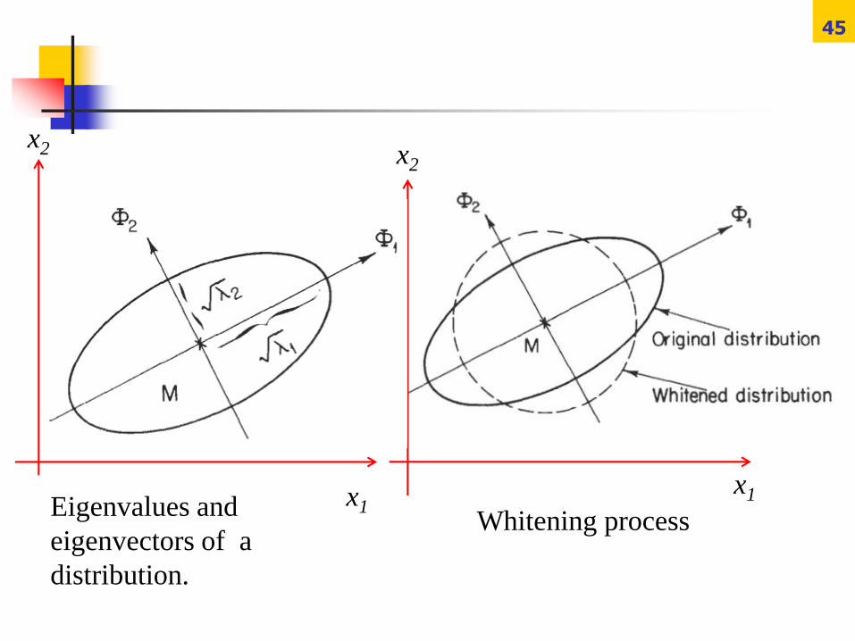
Whitening processEigenvalues and
eigenvectors of a
distribution.
46
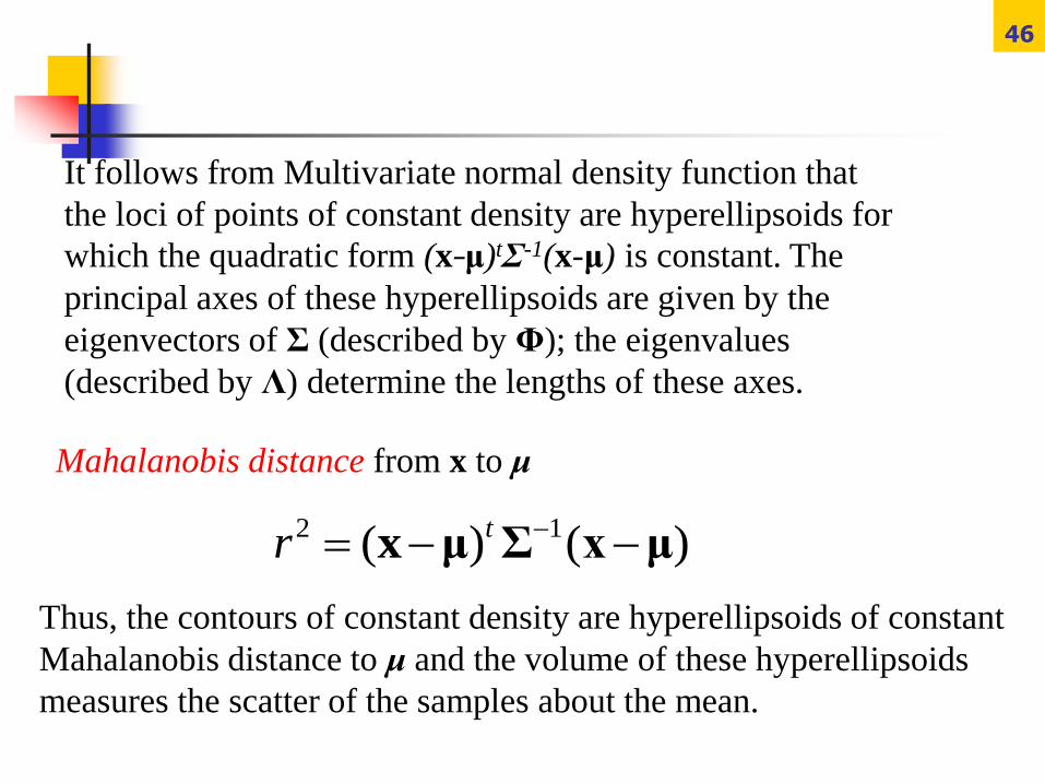
Mahalanobis distance from x to μ
Thus, the contours of constant density are hyperellipsoids of constant
Mahalanobis distance to μ and the volume of these hyperellipsoids
measures the scatter of the samples about the mean.
It follows from Multivariate normal density function that
the loci of points of constant density are hyperellipsoids for
which the quadratic form (x-μ)tΣ-1(x-μ) is constant. The
principal axes of these hyperellipsoids are given by the
eigenvectors of Σ (described by Φ); the eigenvalues
(described by Λ) determine the lengths of these axes.
2 1( ) ( )tr x μ Σ x μ
47
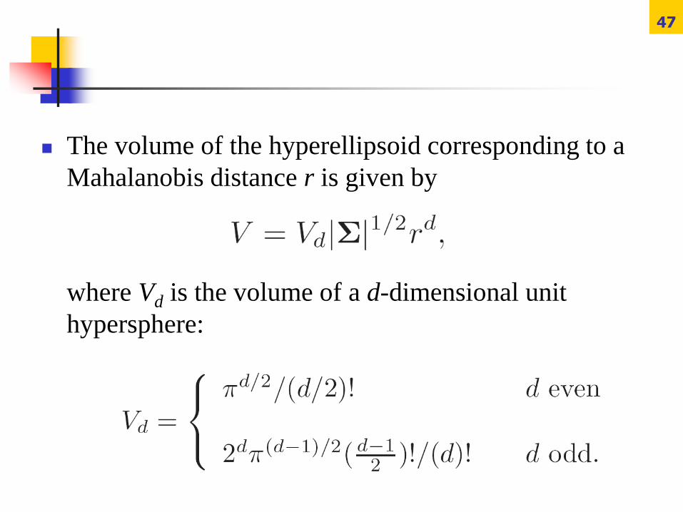
The volume of the hyperellipsoid corresponding to a
Mahalanobis distance r is given by
where Vd is the volume of a d-dimensional unit
hypersphere:
48
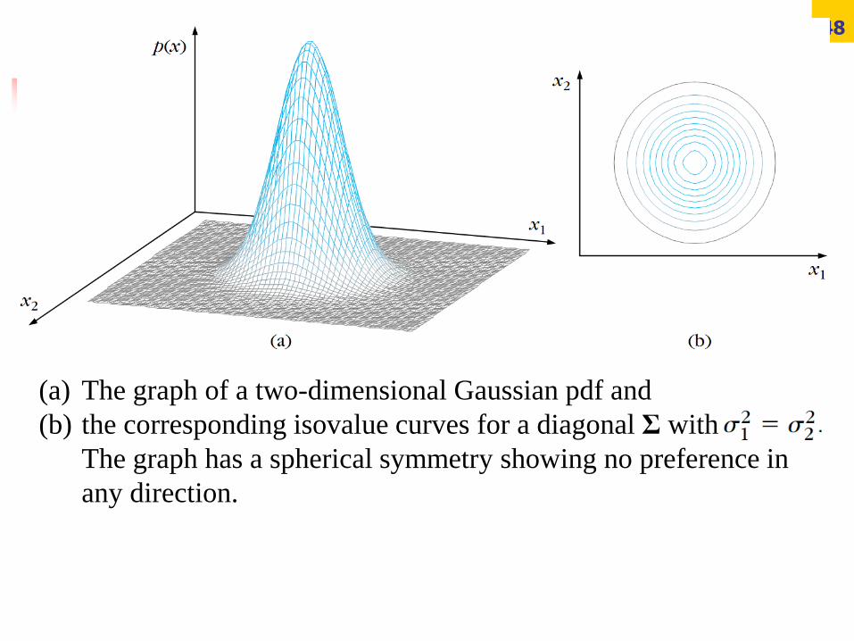
(a) The graph of a two-dimensional Gaussian pdf and
(b) the corresponding isovalue curves for a diagonal Σ with
The graph has a spherical symmetry showing no preference in
any direction.
49
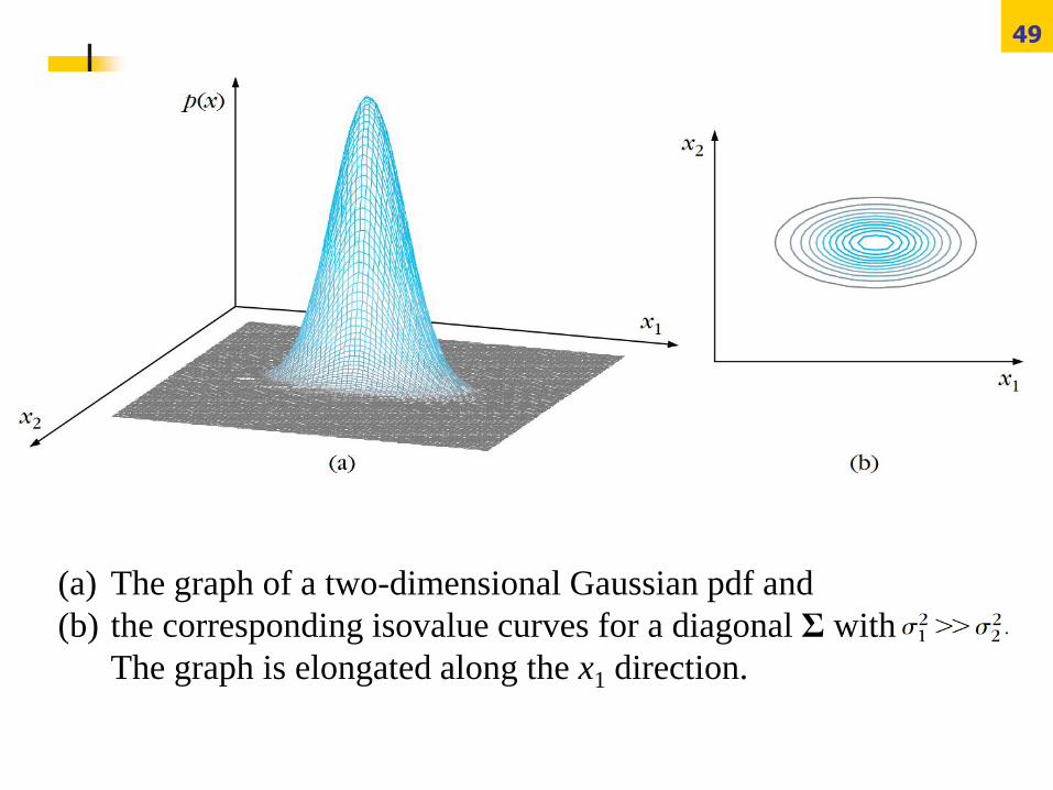
(a) The graph of a two-dimensional Gaussian pdf and
(b) the corresponding isovalue curves for a diagonal Σ with
The graph is elongated along the x1 direction.
50
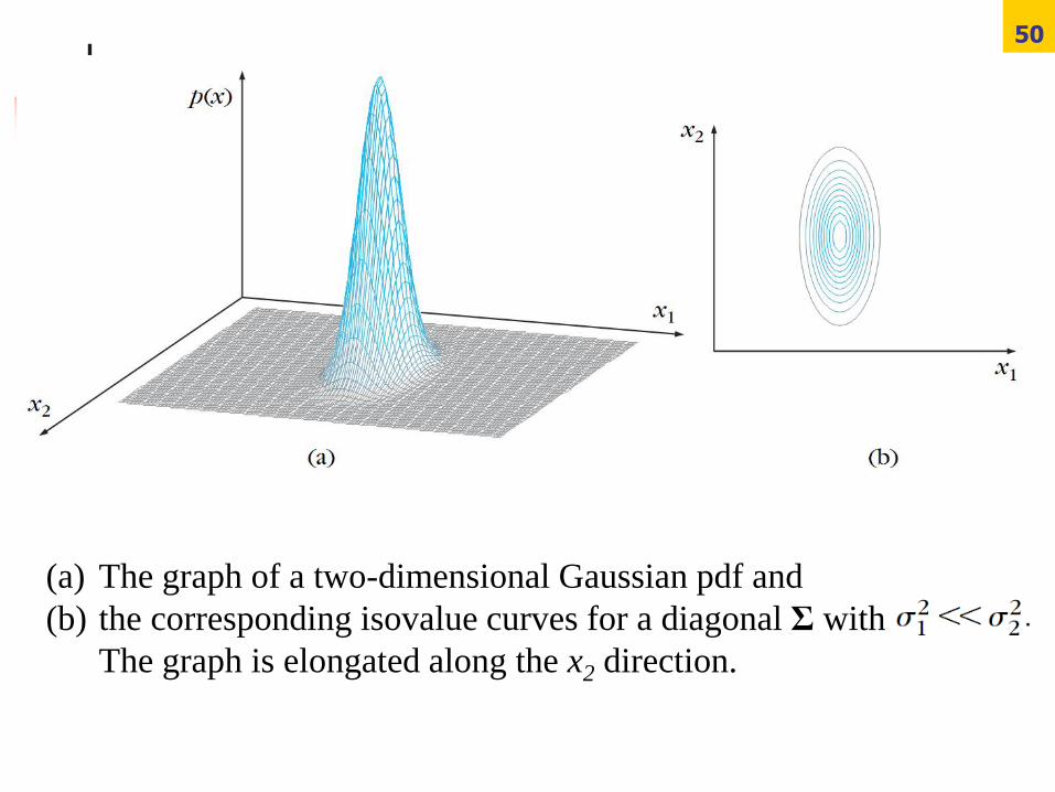
(a) The graph of a two-dimensional Gaussian pdf and
(b) the corresponding isovalue curves for a diagonal Σ with
The graph is elongated along the x2 direction.
51
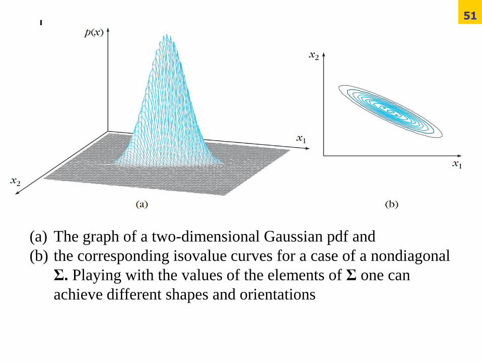
(a) The graph of a two-dimensional Gaussian pdf and
(b) the corresponding isovalue curves for a case of a nondiagonal
Σ. Playing with the values of the elements of Σ one can
achieve different shapes and orientations
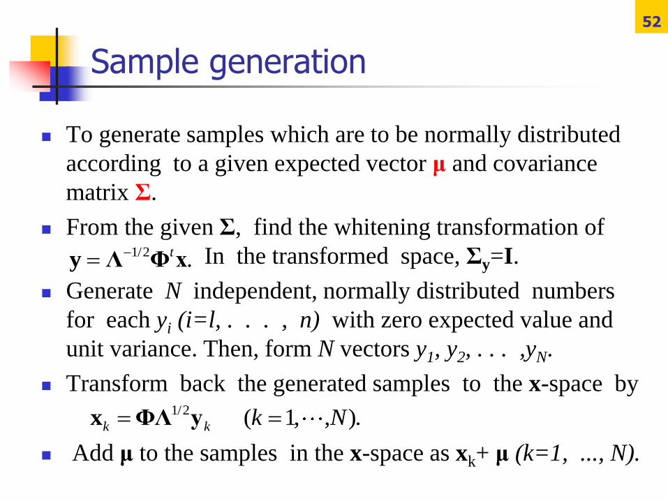
Sample generation
To generate samples which are to be normally distributed
according to a given expected vector μ and covariance
matrix Σ.
From the given Σ, find the whitening transformation of
In the transformed space, Σy=I.
Generate N independent, normally distributed numbers
for each yi (i=l, . . . , n) with zero expected value and
unit variance. Then, form N vectors y1, y2, . . . ,yN.
Transform back the generated samples to the x-space by
Add μ to the samples in the x-space as xk+ μ (k=1, ..., N).
52
1/2 .ty Λ Φ x
1/2 ( 1, , ).k k k N x ΦΛ y