chapter 2 architectures of cognition · 2016-03-05 · 2: architectures of cognition 28 generally,...

CHAPTER 2 Architectures of Cognition

2: Architectures of Cognition

26

2.1 What is an architecture of cognition?

Chapter 1 discussed the single system approach to understanding cognition. This chapter will discuss these systems: architectures of cognition. Cognitive science has borrowed the term architecture from computer science. Computer scientists use the term architecture to refer to the aspects of a computer that are relatively Þxed: the hardware and that part of the software that is Þxed for all applications.

A typical computer architecture has great flexibility: it is capable of executing an infinite variety of programs. However, the architecture can pose constraints on programs. For example, if a computer has a certain amount of memory, it can not run programs that need more memory than is available. The software part of the architecture may also pose constraints. For example, in many time-sharing systems it is impossible to guarantee accurate timing.

Although these limitations may bother many users of computers, they are not interesting for theoretical computer science. In principle, any computer has the same capabilities with respect to what kind of functions it can calculate. This is due to the fact that every computer is equivalent to a universal Turing Machine with respect to the functions it can calculate, except for the fact that a Turing Machine has an infinite memory.

According to the famous Church-Turing thesis (Turing, 1936), a universal Turing Machine can calculate any function that can be calculated at all. A computer architecture is therefore a platform that is ultimately flexible: given the right program, it can calculate any function that is computable in principle, given enough time and memory. The Church-Turing thesis, together with TuringÕs thought experiment called the Turing Test, can be used to argue that human intelligence can be simulated on a computer (Turing, 1950; Taatgen & Andringa, 1997).

Human cognition is also very flexible. Given enough time, it is capable of learning to perform almost any task that is feasible at all for people. An important distinction between computers and people is that people are not programmed in the sense that computers are. On the other hand, people cannot learn new things out of the blue: they almost always need prior knowledge. For example, one cannot learn to add numbers without knowing what numbers are.

This analogy is the basis for the idea of an architecture of cognition. It is the fixed but versatile basis of cognition. The architecture is capable of performing any cognitive task, regardless of the domain the task is from. But where is a cognitive architecture different from a computer architecture, since a computer architecture is already capable of performing any conceivable task? A first difference is that a computer runs a program, and a cognitive architecture a model. On the surface, a model is a kind of program, written in the language of the cognitive architecture. The difference

What is an architecture of cognition?

27

is that a program implements an algorithm, an abstract method to solve a problem. A model is not an algorithm, however, although in some cases it may behave like one. Rather, it specifies the prior knowledge the system has. So, if the model tries to explain the behavior of an expert, the knowledge in it may resemble an algorithm, because experts have effective ways of solving problems. If the model tries to explain novice behavior on the other hand, it can only specify general knowledge. A model of a novice has to discover an effective way to do a task itself, by translating instructions into procedures it can carry out, or by discovering these procedures by itself.

Another difference concerns the way a cognitive architecture is designed. In computer science, the architecture is part of the design of a computer. The architecture is the starting point of the computer. Given the architecture, a VLSI-designer can implement the architecture on a chip, and programmers can write an operating system and other software. If you design a better architecture, you get a better computer. Human cognition is already there, so designing an architecture of cognition serves a different purpose. Designing an architecture of cognition is like specifying a theory, a theory of how cognition works. The quality of a cognitive architecture is not measured in terms of performance, but in terms of the power of the theory it implements. This difference in purpose is the same as the difference between artificial and natural languages. An artificial language is defined by its grammar, while a grammar for a natural language is a theory of the structure of that language.

The starting point for the human cognitive architecture is the brain. But many architectures are more abstract than the architecture of the brain. The main point of discussion is whether or not the grain size of individual neurons is proper for formulating a theory of cognition. According to connectionists, properties of individual neurons are crucial for understanding cognitive performance, and an understanding of how neurons cooperate and learn in different areas of the brain will be the most fruitful route to an understanding of cognition in general. Others, often called symbolists, argue that the level of individual neurons is not the right level to study cognition, and some higher-level representation should be used. The title of Anderson & LebiereÕs 1998 book The Atomic Components of Thought directly refers to this issue. But whatever grain-size we choose, we always abstract away from the biological level of the brain, even if we model neurons in neural networks.

An architecture as a theoryWhat to expect from a cognitive architecture? Since human cognition is complex, a cognitive architecture will have to be able to make complicated predictions. Analytical methods such as the statistics used by most psychologists can be used to make predictions, but are often limited to linear relationships. Cognition is often non-linear, making analytical mathematical methods infeasible. If analytical methods fail, simulation is the next best method to be able to make predictions.


28

Generally, an architecture is an algorithm that simulates a non-linear theory of cognition. This algorithm can be used to make predictions in speciÞc domains and for speciÞc tasks (Figure 2.1).

To be able to make predictions about how people will perform on a specific task, the architecture itself is not enough. Analogous to the computer architecture, where a program is needed to perform tasks, a task model is needed to enable an architecture to simulate something meaningful. Prior knowledge, specified by the model, may be specific to the task, or may be more general. For example, many psychological experiments require the participants to perform some very specific task, such as adding letters as if they were numbers. Such an experiment relies on the fact that participants know how to add numbers and know the order of the alphabet. A model of adding letters would involve knowledge about adding numbers, numbers themselves, letters in the alphabet and knowledge on how to adapt knowledge from one domain to another. It should not incorporate knowledge about adding letters, since it is unreasonable to suppose an average participant in an experiment already has this knowledge. This task-specific knowledge can only be learned during the experiment, or, in the case of the model, during the simulation.

The way task knowledge is merged with the architecture depends on the nature of the architecture. In connectionist theories, all knowledge often has to be learned by a network. To be able to do this, a network has to have a certain topology, some way in which input is fed into the network, and some way to communicate the output. Some types of networks also need some supervisor to provide the network with

Figure 2.1. Relationship between theory, architecture, models and cognition

Architectureof

cognition

CognitionModel of chess

Unified theory of cognition

Model of the blocksworld

Model of language

Model of planning

is simulated by

implements


29

feedback. In neural networks task knowledge is not easy to identify, but is implicit in the environment the network is trained in. In symbolic architectures knowledge is readily identifiable, and consists of the contents of the long-term memory systems the architecture has. Another problem is that it is very hard to give a network any prior knowledge: one always has to start with a system that has no knowledge at all yet. In many cases, this is no problem, but it is in learning complex problem solving, since solving a problem is based to a large extent on prior knowledge.

Regardless of the details, at some point the general theory is combined with task-specific elements to create a task model. A task model is a system that can be used to generate specific predictions about behavior with respect to a certain task. These predictions can be compared to participant data. Figure 2.2 shows the layout of this paradigm. The consequence of this type of research is that the general theory cannot be tested directly. Only the predictions made by task models are tested. If the predictions made by a task model fail to come true, this may be attributed to the architecture, but it may also be attributed to inaccurate task knowledge or the way task knowledge is implemented in the architecture. To be able to judge the achievements of an architecture, there must be some way to generalize over models.

One way to judge the performance of an architecture with respect to a certain task, proposed by Anderson (1993), is to take the best model the architecture can possibly produce for that task. Although this is a convenient way, it is not entirely fair. Suppose we have two architectures, A and B. Given a set of task knowledge, architecture A can only implement a single task model, while architecture B can implement ten task models, nine of which are completely off. Although architecture B may produce the best model, architecture A provides a stronger theory since it only allows for one model.

Architecture (Theory)

Task knowledge

Taskmodel

Predictions Comparison Analyzed data

Analysis

Experiment

Figure 2.2. Research paradigm in cognitive modeling. Adapted from van Someren, Barnard and Sandberg (1994).


30

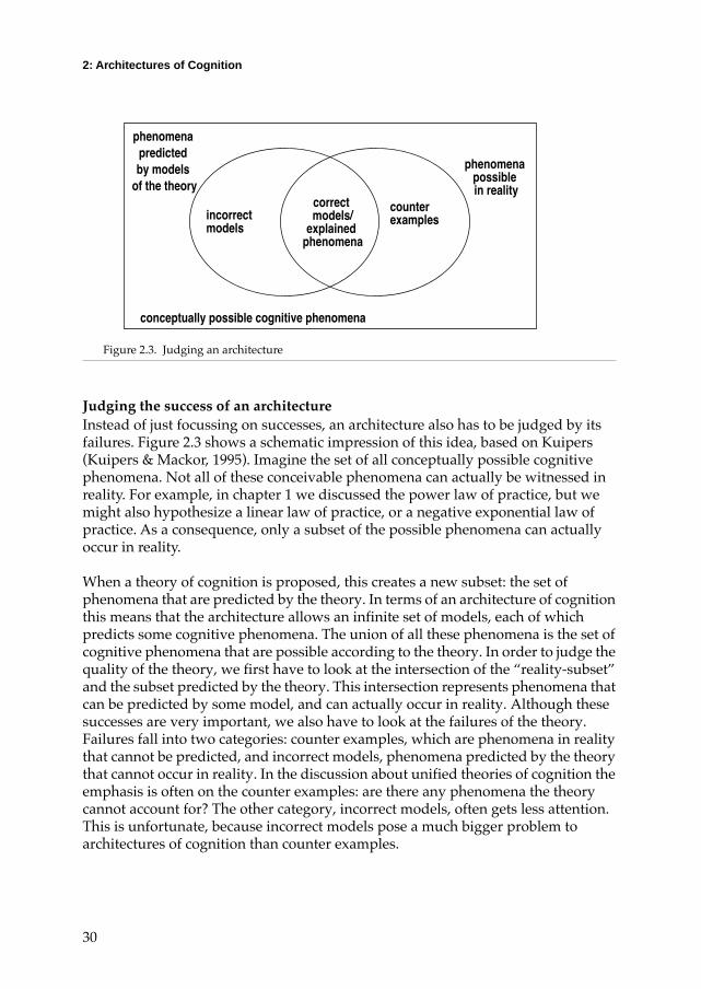
Judging the success of an architectureInstead of just focussing on successes, an architecture also has to be judged by its failures. Figure 2.3 shows a schematic impression of this idea, based on Kuipers (Kuipers & Mackor, 1995). Imagine the set of all conceptually possible cognitive phenomena. Not all of these conceivable phenomena can actually be witnessed in reality. For example, in chapter 1 we discussed the power law of practice, but we might also hypothesize a linear law of practice, or a negative exponential law of practice. As a consequence, only a subset of the possible phenomena can actually occur in reality.

When a theory of cognition is proposed, this creates a new subset: the set of phenomena that are predicted by the theory. In terms of an architecture of cognition this means that the architecture allows an infinite set of models, each of which predicts some cognitive phenomena. The union of all these phenomena is the set of cognitive phenomena that are possible according to the theory. In order to judge the quality of the theory, we first have to look at the intersection of the Òreality-subsetÓ and the subset predicted by the theory. This intersection represents phenomena that can be predicted by some model, and can actually occur in reality. Although these successes are very important, we also have to look at the failures of the theory. Failures fall into two categories: counter examples, which are phenomena in reality that cannot be predicted, and incorrect models, phenomena predicted by the theory that cannot occur in reality. In the discussion about unified theories of cognition the emphasis is often on the counter examples: are there any phenomena the theory cannot account for? The other category, incorrect models, often gets less attention. This is unfortunate, because incorrect models pose a much bigger problem to architectures of cognition than counter examples.

Figure 2.3. Judging an architecture

conceptually possible cognitive phenomena

phenomena

phenomena

correct incorrect

counter

by models predicted

of the theorypossible in reality

modelsmodels/

explained phenomena

examples


31

The reason why incorrect models are a big problem is due to the Church-Turing thesis mentioned earlier. According to this thesis, any computable function can be computed by a general purpose machine such as the Turing Machine. This implies that, theoretically, any sufficiently powerful computer architecture can implement both all possible correct and all possible incorrect models. Figure 2.4 illustrates this implication: a general purpose architecture can, in principle, model any cognitive phenomenon. In terms of a theory of cognition: an ÒemptyÓ theory can predict anything. So, the goal of designing a cognitive architecture is not to give it as much features as possible, but rather to constrain a general purpose architecture as much as possible so that it can only implement correct cognitive models. In practice, as shown in figure 2.4, a typical architecture can produce many incorrect models, but generally produces good models. Constraining the general computer architecture may have an undesired side-effect in the sense that phenomena that could previously be explained are now unreachable.

A cognitive theory in the form of an architecture is not a theory in the sense of Popper (1959), but more like a research program in the sense of Lakatos (1970). According to Popper a good theory is a theory that can be refuted. As we have seen, only predictions by models can be refuted directly. Only the claim that an architecture is an ideal architecture, in the sense of figure 2.4, can be refuted by exposing an incorrect model or producing a counter example. In LakatosÕs view of science, scientists work in research programs. A research program consists of a set of

Figure 2.4. Possible instantiations of Þgure 2.3

predicted = possible

reality

possiblereality =predicted

possible

reality predicted

An arbitrary computer architecture with the power of a universal Turing Machine can model any possible phenomenon

An ideal architecture of cognition only allows models that predict phenomena that can actually occur in reality

Typical architectures cannot exclude all incorrect models, and may not be able to generate models for all phenomena


32

core ideas and a paradigm to do research. The core ideas of a research program are generally not disputed within the program, and researchers will continue working within a certain program as long as the paradigm keeps producing encouraging results. In the research program view, the architecture can be viewed as the core idea of a research program. Creating models of cognitive phenomena is part of the research paradigm. Another part of the research paradigm is a methodology to test models. When is a model considered to be a ÒcorrectÓ model?

Matching model predictions with experimental dataTo consider a model of a cognitive task as a faithful model of human performance, it is not sufÞcient that it can perform the task. A model has to perform the task in the same manner as a participant. In order to be able to make this comparison, we have to compare data from an experiment with the output of a model. Ideally, a model produces data that can be directly compared to participant data. Measures that are used often in psychological experiments are reaction times and accuracies. Models should at least be capable of making predictions in terms of these measures. Some architectures, like ACT-R, are capable of making direct predictions about reaction times. Other architectures only indicate a correspondence between steps or cycles in the system and time. In these type of architectures only relative time between different types of problems or trials can be compared to the data. Accuracy is often measured by the rate of correct responses or by the percentage of items recalled. Not all architectures can model all aspects of accuracy. An architecture like Soar, for example, is only interested in errors that result from incomplete or inconsistent knowledge. So errors due to ÒslipsÓ or forgetting are not considered interesting in the view of the Soar theory.

Since cognitive models give a detailed account of how a task is performed, they make it possible to do more elaborate testing than just reaction times and accuracies. If a trial consists of a number of operations before the response can be given, an attempt can be made to determine the individual latencies of the separate operations, for example by registering eye movement. Reaction times and accuracies tend to change over time, mainly due to learning. The influence of learning can only be disregarded in cases where the task is very simple or the participant is trained exhaustively. Most architectures can account for learning, so should be able to model effects of learning on performance.

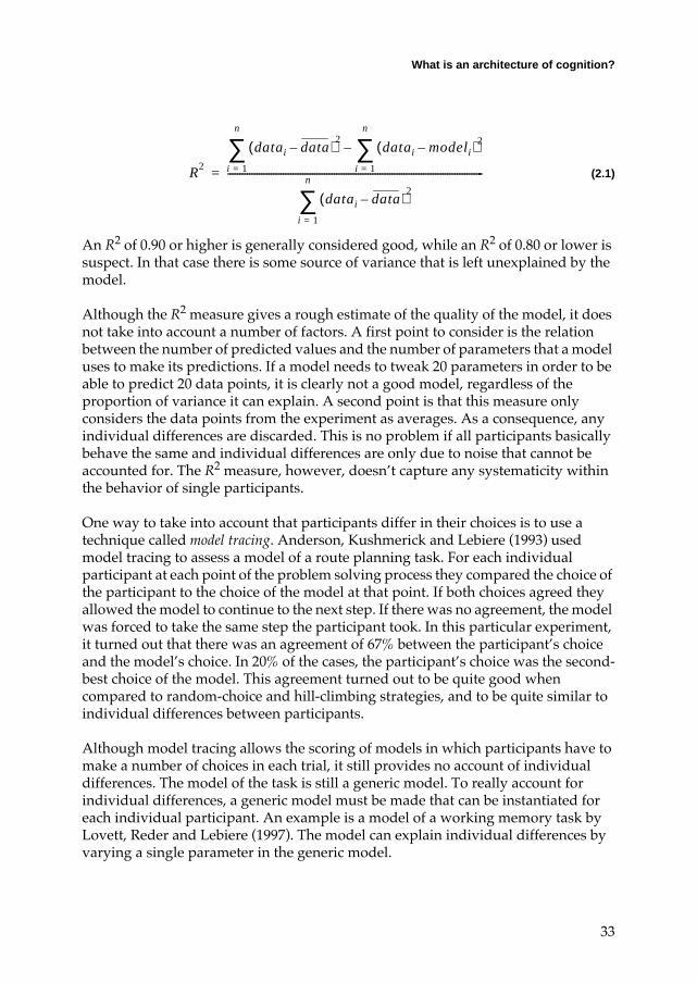
The quality of the predictions of a model is often expressed using the R2 measure, the proportion of variance the model can explain. Suppose we have an experiment that produces n data points, so for example a free-recall experiment in which 20 words can be recalled, we have 20 percentages, one for each of the words, so n=20. The experiment produces data points (datai) that have an average of . The model makes a prediction of these data points (modeli). The explained variance can now be calculated using the following equation:

data


33

(2.1)

An R2 of 0.90 or higher is generally considered good, while an R2 of 0.80 or lower is suspect. In that case there is some source of variance that is left unexplained by the model.

Although the R2 measure gives a rough estimate of the quality of the model, it does not take into account a number of factors. A first point to consider is the relation between the number of predicted values and the number of parameters that a model uses to make its predictions. If a model needs to tweak 20 parameters in order to be able to predict 20 data points, it is clearly not a good model, regardless of the proportion of variance it can explain. A second point is that this measure only considers the data points from the experiment as averages. As a consequence, any individual differences are discarded. This is no problem if all participants basically behave the same and individual differences are only due to noise that cannot be accounted for. The R2 measure, however, doesnÕt capture any systematicity within the behavior of single participants.

One way to take into account that participants differ in their choices is to use a technique called model tracing. Anderson, Kushmerick and Lebiere (1993) used model tracing to assess a model of a route planning task. For each individual participant at each point of the problem solving process they compared the choice of the participant to the choice of the model at that point. If both choices agreed they allowed the model to continue to the next step. If there was no agreement, the model was forced to take the same step the participant took. In this particular experiment, it turned out that there was an agreement of 67% between the participantÕs choice and the modelÕs choice. In 20% of the cases, the participantÕs choice was the second-best choice of the model. This agreement turned out to be quite good when compared to random-choice and hill-climbing strategies, and to be quite similar to individual differences between participants.

Although model tracing allows the scoring of models in which participants have to make a number of choices in each trial, it still provides no account of individual differences. The model of the task is still a generic model. To really account for individual differences, a generic model must be made that can be instantiated for each individual participant. An example is a model of a working memory task by Lovett, Reder and Lebiere (1997). The model can explain individual differences by varying a single parameter in the generic model.

R2

datai data–( )2

datai modeli–( )2

i 1=

n

∑–i 1=

n

∑

datai data–( )2

i 1=

n

∑----------------------------------------------------------------------------------------------------------=


34

In summary, a good model is a model that can approximate as many data points as possible using as few parameters as possible. In tasks with large individual differences, a model that can explain individual differences by varying parameters is better than a model that reproduces averages.

2.2 An overview of current architectures

In this section I will review four popular architectures of cognition, all of which have been reasonably successful in modeling various cognitive phenomena. The four architectures to be discussed, Soar, EPIC, 3CAPS and ACT-R, are all either pure symbolic or hybrid architectures. This means all of them share the idea that symbols are the right grain-size to study cognition. However, a pure symbolic theory assumes the underlying neural structure is irrelevant, while a hybrid theory argues that subsymbolic processing plays an important role.

SoarThe Soar (States, Operators, And Reasoning) architecture, developed by Laird, Rosenbloom and Newell (1987; Newell, 1990; Michon & Aky�rek, 1992), is a descendant of the General Problem Solver (GPS), developed by Newell and Simon (1963). Human intelligence, according to the Soar theory, is an approximation of a knowledge system. Newell deÞnes a knowledge system as follows (Newell, 1990, page 50):

A knowledge system is embedded in an external environment, with which it interacts by a set of possible actions. The behavior of the system is the sequence of actions taken in the environment over time. The system has goals about how the environment should be. Internally, the system processes a medium, called knowledge. Its body of knowledge is about its environment, its goals, its actions, and the relations between them. It has a single law of behavior: the system takes actions to attain its goals, using all the knowledge that it has. This law describes the results of how knowledge is processed. The system can obtain new knowledge from external knowledge sources via some of its actions (which can be called perceptual actions). Once knowledge is acquired it is available forever after. The system is a homogeneous body of knowledge, all of which is brought to bear on the determination of its actions. There is no loss of knowledge over time, though of course knowledge can be communicated to other systems.

According to this definition, the single important aspect of intelligence is the fact that a system uses all available knowledge. Errors due to lack of knowledge are no failure of intelligence, but errors due to a failure in using available knowledge are. Both human cognition and the Soar architecture are approximations of an ideal intelligent knowledge system. As a consequence, properties of human cognition that are not

An overview of current architectures

35

part of the knowledge system approach are not interesting, and are not accounted for by the Soar architecture.

The Soar theory views all intelligent behavior as a form of problem solving. The basis for a knowledge system is therefore the problem-space computational model (PSCM), a framework for problem solving based on the weak-method theory discussed in chapter 1. In Soar, all tasks are represented by problem spaces. Performing a certain task corresponds to reaching the goal in a certain problem space. As we have seen in chapter 1, the problem solving approach has a number of problems. To be able to find the goal in a problem space, knowledge is needed about all possible operators, about consequences of operators and about how to choose between operators if there is more than one available. SoarÕs solution to this problem is to use multiple problem spaces. If a problem, ÒimpasseÓ in Soar terms, arises due to the fact that certain knowledge is lacking, resolving this impasse automatically becomes the new goal. This new goal becomes a subgoal of the original goal, which means that once the subgoal is achieved, control is returned to the main goal. The subgoal has its own problem space, state and possible set of operators. Whenever the subgoal has been achieved it passes its results to the main goal, thereby resolving the impasse. Learning is also keyed to the subgoaling process: whenever a subgoal has been achieved, new knowledge is added to the knowledge base to prevent the impasse that produced the subgoal from occurring again. So, if an impasse occurs because the consequences of an operator are unknown, and in the subgoal these consequences are subsequently found, knowledge is added to SoarÕs memory about the consequences of that operator.

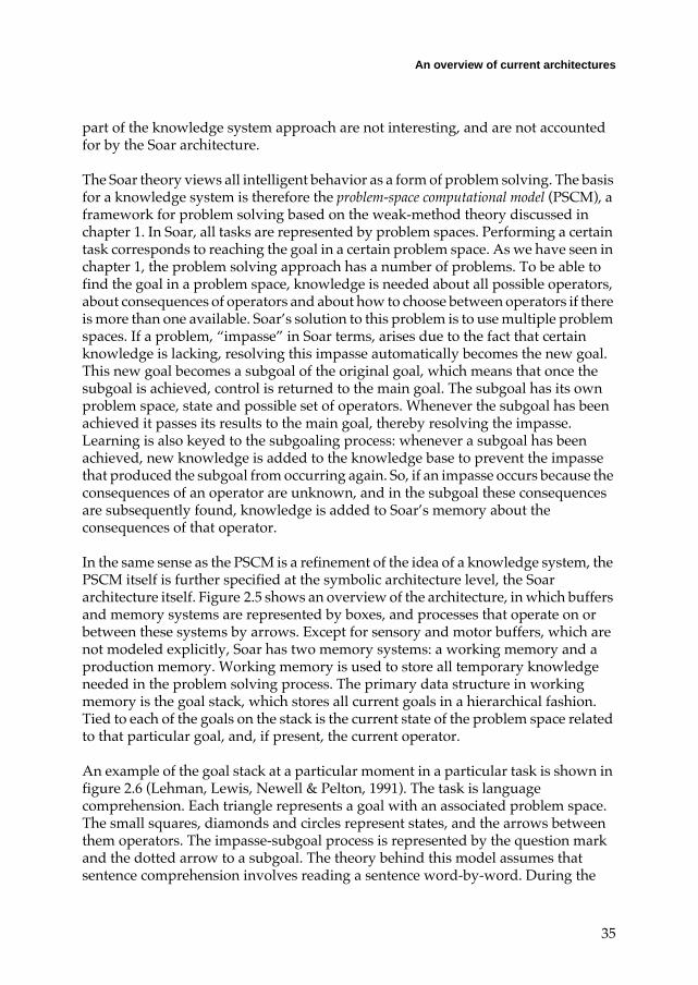
In the same sense as the PSCM is a refinement of the idea of a knowledge system, the PSCM itself is further specified at the symbolic architecture level, the Soar architecture itself. Figure 2.5 shows an overview of the architecture, in which buffers and memory systems are represented by boxes, and processes that operate on or between these systems by arrows. Except for sensory and motor buffers, which are not modeled explicitly, Soar has two memory systems: a working memory and a production memory. Working memory is used to store all temporary knowledge needed in the problem solving process. The primary data structure in working memory is the goal stack, which stores all current goals in a hierarchical fashion. Tied to each of the goals on the stack is the current state of the problem space related to that particular goal, and, if present, the current operator.

An example of the goal stack at a particular moment in a particular task is shown in figure 2.6 (Lehman, Lewis, Newell & Pelton, 1991). The task is language comprehension. Each triangle represents a goal with an associated problem space. The small squares, diamonds and circles represent states, and the arrows between them operators. The impasse-subgoal process is represented by the question mark and the dotted arrow to a subgoal. The theory behind this model assumes that sentence comprehension involves reading a sentence word-by-word. During the


36

ProductionMemory

WorkingMemory

Perceptual Systems

MotorSystems

Senses Muscles

ExecutionChunking

Decision

Match

Figure 2.5. Overview of the Soar architecture (from Newell, Rosenbloom & Laird, 1989)

Figure 2.6. Example of the goal stack in Soar in a language comprehension model (from Lehman, Lewis, Newell and Pelton, 1991).

Top problem spaceTwo alternating operators: comprehend a word and attend the next word

Language spaceTry to update the current interpretation of the sentence in accordance with the new word

Constraint spaceTry to find syntactic and semantic constraints to restrain the number of choices

Semantics spaceTry to find general world knowledge to further constrain choices


37

reading process a representation of the meaning of the sentence is assembled. So, at the top problem space, the goal is to comprehend a sentence. This goal is accomplished by alternating two operators: an attend operator, which reads the next word, and a comprehension operator, which augments or updates the current interpretation of the sentence. Comprehending a word is generally not possible in a single step, so after the comprehend operator is selected, an impasse will occur. This impasse generates the language subgoal, which tries to update the current interpretation of a sentence given a new word. The language subgoal has several operators to do this. A word can simply be linked in the interpretation. Sometimes a new word refers to a word read earlier, making it necessary to find the word referred to. In other cases the interpretation built earlier is wrong, and has to be reconstructed. The language space often offers too many choices to link words to each other, so a third subgoal, the constraint goal, is needed to create constraints on the possible linkings. This constraint space uses syntactic and semantic constraints to help making the choice. To find semantic constraints, it is sometimes necessary to use general world knowledge, which is found using the fourth and final subgoal, the semantics goal.

All knowledge needed for problem solving is stored in production memory in the form of rules. Although all knowledge is stored in production rules, they do not have the same active role production rules usually have. A rule in Soar cannot take actions by itself, it may only propose actions. So if Soar is working on a certain goal and is in a certain state, rules may propose operators that may be applied in the current state. Other rules may then evaluate the proposed operators, and may add so-called preferences to them, for example stating that operator A is better than operator B. The real decisions are made by the decision mechanism. The decision mechanism examines the proposals and decides which proposal will be executed. The decision mechanism is actually quite simple. If it is possible to make an easy decision, for example if there is just one proposal or preferences indicate a clear winner, it makes this decision, else it observes an impasse has been reached and creates a subgoal to resolve this impasse. So, the problem of choice in Soar is not handled at the level of individual production rule firings, which are allowed to occur in parallel, but at the level of the proposals of change made by these rules. The learning mechanism in Soar is called chunking.

As mentioned before, learning is keyed to impasses and subgoaling. Whenever a subgoal is popped from the goal stack, Soar creates a new production rule with a generalization of the state before the impasse occurred as the condition, and the results of the subgoal as the action. Dependent on the nature of the impasse, this new rule may propose new operators, create preferences between operators, or implement operators or do other things.

In the language comprehension example discussed earlier learning occurs at all levels of the model. At the level of the comprehension problem space, Soar may learn


38

a production rule that implements the comprehension operator for a specific word in a specific context. But Soar may also learn a production rule in the constraints problem space to generate a semantic constraint on possible meanings of a sentence.

The knowledge system approach of Soar has a number of consequences. Because not all aspects of human cognition are part of the knowledge system approximation, some aspects will not be part of the Soar theory, although they contribute to human behavior as witnessed in empirical data. Another property of the Soar system is that all choices are deliberate. Soar will never make an arbitrary choice between operators, it either knows which operator is best, or it will try to reason it out. Since intelligence, according to the knowledge system definition, can only involve choosing the optimal operator based on the current knowledge, it does not say much about what the system has to do in the case of insufficient knowledge.

An aspect of human memory that is not modeled in Soar is forgetting. According to the knowledge-system view this is a deviation from ideal intelligence, a weakness of the human mind. This rules out the possibility that forgetting has a function, for example to purge the memory from useless information, allowing for better access to useful information. An error such as choosing a sub-optimal strategy is also considered as aberration of rationality, and is therefore not part of Soar. To sometimes favor a sub-optimal strategy over the optimal strategy may on the other hand have advantages. Maybe one of the sub-optimal strategies has improved due to an increase in knowledge or a change in the environment, and has become the optimal theory. In many situations, the only way to discover how optimal a strategy is, is to just try it sometimes.

Since SoarÕs behavior deviates from human behavior with respect to aspects that are not considered rational by the Soar theory, the Soar architecture can only make predictions about human behavior in situations where behavior is not too much influenced by ÒirrationalÓ aspects. Another consequence of the fact that Soar only models rational aspects of behavior is the fact that its predictions are only approximate. An example is SoarÕs predictions about time. A decision cycle in Soar takes Ò~~100 msÓ, where Ò~~Ó means Òmay be off by a factor of 10Ó. So in a typical experiment SoarÕs predictions have to be determined in terms of the number of decision cycles needed, while the data from the experiment have to be expressed in terms of reaction times. If both types of data show the same characteristics, for example if both show the power law of practice, a claim of correspondence can be made.

One of the strong points of Soar is its parsimony. Soar has a single long-term memory store, the production memory, and a single learning mechanism, chunking. Soar also adheres to a strict symbolic representation. The advantage of parsimony is that it provides a stronger theory. For example, since chunking is the only learning mechanism, and chunking is tied to subgoaling, Soar predicts that no learning will


39

occur if there are no impasses. In a sense Soar sets an example: if one wants to propose an architecture with two long-term memory stores, one really has to show that it can not be done using just one.

ACT-RThe ACT-R (Adaptive Control of Thought, Rational) theory (Anderson, 1993; Anderson & Lebiere, 1998) rests upon two important components: rational analysis (Anderson, 1990) and the distinction between procedural and declarative memory (Anderson, 1976). According to rational analysis, each component of the cognitive architecture is optimized with respect to demands from the environment, given its computational limitations. If we want to know how a particular aspect of the architecture should function, we Þrst have to look at how this aspect can function as optimal as possible in the environment. Anderson (1990) relates this optimality claim to evolution. An example of this principle is the way choice is implemented in ACT-R. Whenever there is a choice between what strategy to use or what memory element to retrieve, ACT-R will take the one that has the highest expected gain, which is the choice that has the lowest expected cost while having the highest expected probability of succeeding.

The principle of rational analysis can also be applied to task knowledge. While evolution shapes the architecture, learning shapes the knowledge and parts of the knowledge acquisition process. Instead of only being focused on acquiring knowledge per se, learning should also aim at finding the right representation. This may imply that learning has to attempt several different ways to represent knowledge, so that the optimal one can be selected.

Both Soar and ACT-R claim to be based on the principles of rationality, although they define rationality differently. In Soar rationality means making optimal use of the available knowledge to attain the goal, while in ACT-R rationality means optimal adaptation to the environment. Not using all the knowledge available is irrational in Soar, although it may be rational in ACT-R if the costs of using all knowledge are too high. On the other hand ACT-R takes into account the fact that its knowledge may be inaccurate, so additional exploration is rational. Soar cannot handle the need for exploration very well, since that would imply that currently available knowledge is not used to its full extent.

The distinction between procedural and declarative memory is studied quite extensively in psychology. Although one should be careful to map distinctions from psychology onto cognitive architectures directly, the best way to explain this distinction is to assume different representations and different memory systems. The disadvantage of this differentiation is that the architecture becomes less simple than an architecture with only a single memory system, like Soar. On the other hand, ACT-R has no separate working memory and instead uses declarative memory in conjunction with an activation concept to store short-term facts. To keep track of the


40

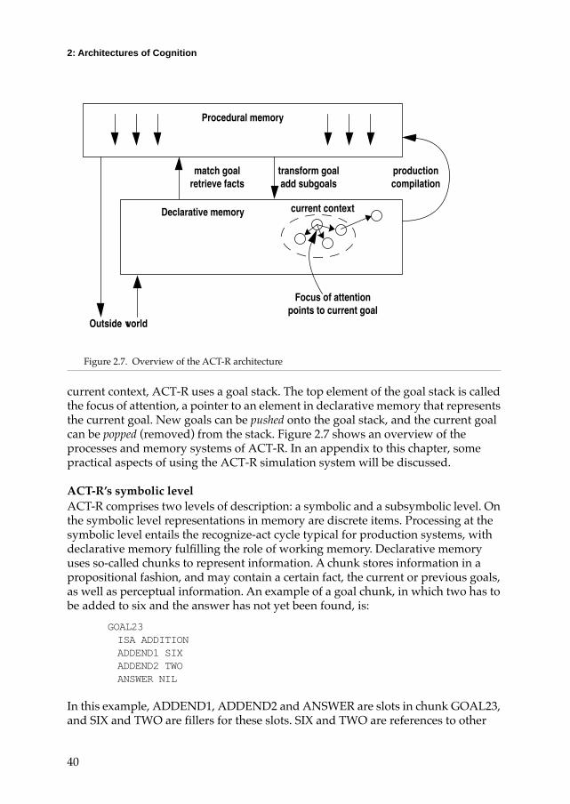
current context, ACT-R uses a goal stack. The top element of the goal stack is called the focus of attention, a pointer to an element in declarative memory that represents the current goal. New goals can be pushed onto the goal stack, and the current goal can be popped (removed) from the stack. Figure 2.7 shows an overview of the processes and memory systems of ACT-R. In an appendix to this chapter, some practical aspects of using the ACT-R simulation system will be discussed.

ACT-RÕs symbolic levelACT-R comprises two levels of description: a symbolic and a subsymbolic level. On the symbolic level representations in memory are discrete items. Processing at the symbolic level entails the recognize-act cycle typical for production systems, with declarative memory fulÞlling the role of working memory. Declarative memory uses so-called chunks to represent information. A chunk stores information in a propositional fashion, and may contain a certain fact, the current or previous goals, as well as perceptual information. An example of a goal chunk, in which two has to be added to six and the answer has not yet been found, is:

GOAL23ISA ADDITIONADDEND1 SIXADDEND2 TWOANSWER NIL

In this example, ADDEND1, ADDEND2 and ANSWER are slots in chunk GOAL23, and SIX and TWO are fillers for these slots. SIX and TWO are references to other

current context

Procedural memory

production compilation

Figure 2.7. Overview of the ACT-R architecture

Outside world

Declarative memory

Focus of attentionpoints to current goal

match goalretrieve facts

transform goaladd subgoals


41

chunks in declarative memory. The ANSWER slot has a value of NIL, meaning the answer is not known yet.

Assume that this chunk is the current goal. If ACT-R manages to fill the ANSWER slot and focuses its attention on some other goal, GOAL23 will become part of declarative memory and takes the role of the fact that six plus two equals eight. Later, this fact may be retrieved for subsequent use.

Procedural information is represented in production memory by production rules. A production rule has two main components: the condition-part and the action-part. The condition-part contains patterns that match the current goal and possibly other elements in declarative memory. The action-part can modify slot-values in the goal and can create subgoals (and some other actions we will not discuss in detail here). A rule that tries to solve a subtraction problem by retrieving an addition chunk might look like:

IF the goal is to subtract num2 from num1 and there is no answerAND there is a addition chunk num2 plus num3 equals num1

THEN put num3 in the answer-slot of the goal

This example also shows an important aspect of production rules, namely variables. Num1, num2 and num3 are all variables that can be instantiated by any value. So this rule can find the answer to any subtraction problem, if the necessary addition chunk is available.

ACT-RÕs subsymbolic levelThe symbolic level provides the basic building blocks of ACT-R. Using this level only already allows for several interesting models for tasks in which a clearly deÞned set of rules has to be applied. The symbolic level leaves a number of details unspeciÞed, however. The main topic that it delegates to the subsymbolic level is choice. Choices must be made when there is more than one production rule that can match, or when there is more than one chunk that matches a pattern in a production rule. Other matters that are taken care of by the subsymbolic level are accounts for errors and forgetting, as well as the prediction of latencies.

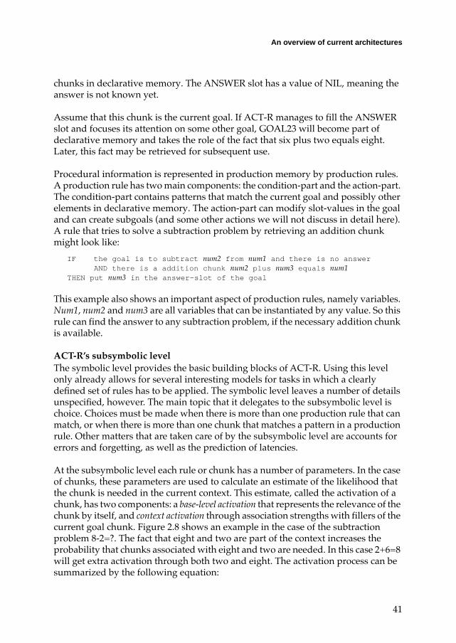
At the subsymbolic level each rule or chunk has a number of parameters. In the case of chunks, these parameters are used to calculate an estimate of the likelihood that the chunk is needed in the current context. This estimate, called the activation of a chunk, has two components: a base-level activation that represents the relevance of the chunk by itself, and context activation through association strengths with fillers of the current goal chunk. Figure 2.8 shows an example in the case of the subtraction problem 8-2=?. The fact that eight and two are part of the context increases the probability that chunks associated with eight and two are needed. In this case 2+6=8 will get extra activation through both two and eight. The activation process can be summarized by the following equation:


42

(2.2)

In this equation, Ai is the total activation of chunk i. This total activation has two parts, a relatively Þxed base-level activation (Bi) and a variable part determined by the context (the summation). The summation adds up the inßuences for each of the elements in the current context. Whether or not a chunk is part of the current context is represented by Wj: if a chunk is part of the context, Wj=W/n, otherwise Wj=0. n is the total number of chunks in the context and W is some Þxed ACT-R parameter which usually has a value of 1. The Sji values represent the association strengths between chunks.

The activation level of a chunk has a number of consequences for its processing. If there is more than one chunk that matches the pattern in a production rule, the chunk with the highest activation is chosen. Differences in activation levels can also lead to mismatches, in which a chunk with a high activation that does not completely match the production rule is selected. Such a chunk can be matched anyway, at an activation penalty, by a process called partial matching. Finally activation plays a role in latency: the lower the activation of a chunk is, the longer it takes to retrieve it. This retrieval time is calculated using the following equation:

(2.3)

Since a chunk is always retrieved by a production rule, this equation expresses the time to retrieve chunk i by production rule p. Besides the activation of the chunk, the strength of the production rule (Sp) also plays a role. The F and f parameters are Þxed ACT-R parameters, both of which default to 1. As the sum of activation and

Goal405Subtraction

Goal23Addition

Two

Six

Eight

Nil

Current context

Figure 2.8. Example of spreading activation in ACT-R. The current goal is Goal405, which represents the subtraction problem 8-2=?. The context consists of Goal405 and the numbers eight and two. Context elements are sources of spreading activation. In this example they give extra activation to Goal23, an addition fact that can be used to Þnd the answer to the subtraction. Spreading activation is indicated by dotted arrows.

Ai Bi W jS ji noise+j

∑+=

Timeip Fef Ai Sp+( )–

=


43

strength decreases, the time to retrieve a chunk grows exponentially. To avoid retrieval times that exceed the order of a second, a retrieval threshold is deÞned. Chunks with an activation value below the threshold cannot be retrieved.

Choices between production rules are determined by estimates of their expected gain. To be able to calculate the expected gain of a certain rule, several parameters are used to make an estimate. The main equation that governs this estimate is:

(2.4)

In this equation is the estimated probability of reaching the goal using production rule p, G is the value of the goal, and the estimated cost of reaching the goal using p. The unit of cost in ACT-R is time. Suppose we are willing to spend 10 seconds on a certain goal (G=10), and suppose there are two production rules p1 and p2, and p1 reaches the goal 60% of the time ( ) in 2 seconds on average ( ). Similarly, and . In that case the expected gain of p1 is 4, and the expected gain of p2 is 3. So, p1 is selected in favor of p2, since its expected gain is higher. To be able to estimate all these values, ACT-R maintains a number of parameters with each production rule. Besides parameters to calculate the expected gain, production rules also have a strength parameter, comparable to activation of chunks. The strength parameter is another component that determines the latency of firing a production: productions with a higher strength take less time to match (equation 2.3).

Learning in ACT-RWhile ACT-R has two distinct memory systems with two levels of description, distinct learning mechanisms are proposed to account for the knowledge that is represented as well as for its parameters. At the symbolic level, learning mechanisms specify how new chunks and rules are added to declarative and procedural memory. At the subsymbolic level, learning mechanisms change the values of the parameters. Objects are never removed from memory, although they may become virtually irretrievable.

A new chunk in declarative memory has two possible sources: it either is a perceptual object, or a chunk created internally by the goal processing of ACT-R itself. ACT-RÕs internally created chunks are always old goals, as exemplified by the ADDITION-goal discussed earlier. Any chunk in declarative memory that has not originated from perception has once been the current goal in ACT-R.

Learning new production rules is a more intricate process. Production rules are learned from examples. These examples are structured in the form of a dependency chunk. A dependency is a special type of chunk, which points to all the necessary components needed to assemble a production rule. Figure 2.9 shows the dependency structure necessary for the subtraction rule. In this example, three slots

Estimated Gain for production p PpG C p–=

PpC p

Pp1 0.6=C p1 2= Pp2 0.8= C p2 5=


44

of the dependency are filled: the goal slot contains an example of a goal in which the answer slot is still empty (nil), and the modified slot has an example of the same goal, but now with its answer slot filled. The constraints slot contains the fact that has been used to transform the original goal into the modified goal. Since a dependency is a chunk that obviously is not a perceptual chunk, it must be an old goal. In order to learn a new rule, a dependency goal must be pushed onto the goal-stack. After processing, the dependency is popped and the production compilation mechanism (in former versions of ACT-R called analogy) generalizes the dependency to a production rule. This scheme for production rule learning has two important properties: it is dependent on declarative memory, and assembling a rule is a goal-driven process.

Since the parameters at the subsymbolic level estimate properties of certain knowledge elements, learning at this level is aimed at adjusting the estimates in the light of experience. The general principle guiding these estimates is the well known BayesÕ Theorem (Berger, 1985). According to this principle, a new estimate for a parameter is based on its prior value and the current experience.

The base-level activation of a chunk estimates the probability that it is needed, regardless of the current context. If a chunk was retrieved a number of times in the immediate past, the probability that it will be needed again is relatively high. If a chunk has not been retrieved for a long time, the probability that it will be needed now is only small. So, each time a chunk is retrieved, its base-level activation should

Dependency

AdditionSubtraction goal

with solutionOriginal

subtraction goalNil

Eight Six Two

Figure 2.9. Example of the declarative structure needed to learn the subtraction production. In this case, the dependency has three Þlled slots: the original goal, the modiÞed goal in which the answer slot is Þlled, and a constraint, an old addition goal that was used to calculate the answer

goal modified constraints

arg1 arg1arg2arg2

answer

answer addend1addend2

sum


45

go up, and each time it is not used, it should go down. This is exactly what the base-level learning mechanism does: it increases the base-level activation of a chunk each time it is retrieved, and causes it to decay over time. The following equation calculates the base-level activation of a chunk:

(2.5)

In this formula, n is the number of times a chunk has been retrieved from memory, and represents the time at which each of these retrievals took place. So, the longer ago a retrieval was, the less it contributes to the activation. d is a fixed ACT-R parameter that represents the decay of base-level activation in declarative memory (default value=0.5).

The other parameters are estimated in a similar fashion. For example, the probability of success of a production rule goes up each time it leads successfully to a goal, and goes down each time the rule leads to failure.

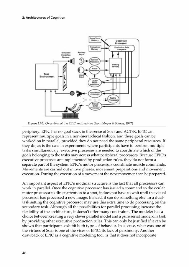
EPICSoar and ACT-R focus on central cognition. The EPIC (Executive-Process Interactive Control) architecture (Meyer & Kieras, 1997) instead stresses the importance of peripheral cognition as a factor that determines task performance. This stress on peripheral cognition is immediately apparent in the overview of EPIC in Þgure 2.10. Except for the cognitive processor with its associated memory systems, the main focus of the other three architectures discussed in this chapter, EPIC provides a set of detailed perceptual and motor processors. In order to study the role of perceptual and motor processors, it is also necessary to simulate a highly detailed task environment. The perceptual modules are capable of processing stimuli from simulated sensory organs, sending their outputs to working memory. They operate asynchronously, and the time they require to process an input depends on the modality, intensity and discriminability of the stimulus. The time requirements of the perceptual modules, as well as other modules, are relatively Þxed, and serve as an important source of constraints.

EPICÕs cognitive processor is a parallel matcher: in each cycle, which takes 50 ms, production rules are matched to the contents of working memory. Each rule that matches is allowed to fire, so there is no conflict resolution. It is up to the modeler to prevent this parallel firing scheme from doing the wrong thing. Whereas both Soar and ACT-R have a production firing system that involves both parallel and serial aspects, EPIC has a pure parallel system of central cognition. As a consequence, EPIC predicts that serial aspects of behavior are mainly due to communication between central and peripheral processors and structural limitations of sense organs and muscles. Corresponding to this idea that processing bottlenecks are located in the

Bi t( ) t t– j( ) d–

j 1=

n

∑log=

t j


46

periphery, EPIC has no goal stack in the sense of Soar and ACT-R. EPIC can represent multiple goals in a non-hierarchical fashion, and these goals can be worked on in parallel, provided they do not need the same peripheral resources. If they do, as is the case in experiments where participants have to perform multiple tasks simultaneously, executive processes are needed to coordinate which of the goals belonging to the tasks may access what peripheral processors. Because EPICÕs executive processes are implemented by production rules, they do not form a separate part of the system. EPICÕs motor processors coordinate muscle commands. Movements are carried out in two phases: movement preparations and movement execution. During the execution of a movement the next movement can be prepared.

An important aspect of EPICÕs modular structure is the fact that all processors can work in parallel. Once the cognitive processor has issued a command to the ocular motor processor to direct attention to a spot, it does not have to wait until the visual processor has processed a new image. Instead, it can do something else. In a dual-task setting the cognitive processor may use this extra time to do processing on the secondary task. Although all the possibilities for parallel processing increase the flexibility of the architecture, it doesnÕt offer many constraints. The modeler has a choice between creating a very clever parallel model and a pure serial model of a task by providing other executive production rules. This can only be justified if it can be shown that participants exhibit both types of behavior. In a sense, what was one of the virtues of Soar is one of the vices of EPIC: its lack of parsimony. Another drawback of EPIC as a cognitive modeling tool, is that it does not incorporate

Figure 2.10. Overview of the EPIC architecture (from Meyer & Kieras, 1997)


47

learning. As has been discussed in chapter 1, it can be doubted whether information processing and learning can be studied separately.

3CAPSWhile EPIC proposes that most constraints posed on the architecture are due to structural limitations of sense organs and muscles, 3CAPS (Just & Carpenter, 1992) proposes limitations on working-memory capacity as the main source of constraints. 3CAPS has a working memory, a declarative memory and a procedural memory. As in ACT-R, memory elements have activation values. As long as the activation of an element is above a certain threshold, it is considered part of working memory and can be accessed by production rules. Capacity theory, 3CAPSÕs foundation, speciÞes that a certain amount of activation units is available. These activation units can be used to either keep elements active in working memory or to propagate activation by Þring production rules. If the maximum amount is reached, both working memory maintenance and production Þring processes get less activation units than they need. The result of activation deprivation for working memory is that memory elements may be forgotten prematurely. If processing gets less activation than needed, production rules have to Þre multiple times to get the activations of target working memory elements above the threshold, effectively slowing it down.

The 3CAPS theory views the limitation in activation units as a source of individual differences. It has been successful in explaining individual differences in language comprehension, relating performance differences in reading and comprehending sentences to working memory span (Just & Carpenter, 1992). A limitation of 3CAPS is that it does not incorporate learning.

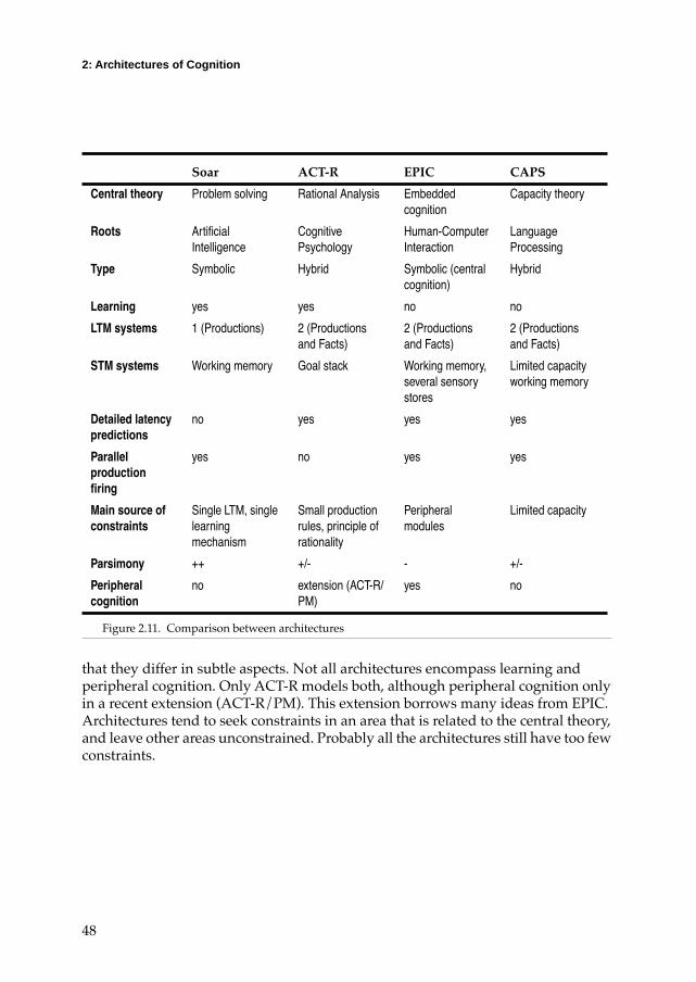
A summary of the four architecturesFigure 2.11 summarizes the properties of the four architectures discussed in this section. Each of the architectures has its own central theory, and its own roots. Most of the architectures settle on two long-term memory stores, one for procedures and one for facts. All of them have some form of working memory, although in the case of ACT-R this is only a goal stack with pointers to declarative memory. Both ACT-R and 3CAPS have an activation-based mechanism to represent availability of memory elements. Although the mechanisms behind them differ, they share some characteristics. 3CAPS poses a strict activation limit. The consequence of exceeding the limit is forgetting and longer reaction times. These consequences, however, also concur with ACT-RÕs effects of low activation. If the current context in ACT-R contains many elements, spreading activation is divided over all these elements, resulting in lower activation of associated elements. Although there is no explicit activation limit in ACT-R, thinning out activation may lead to a sudden decrease in performance when elements drop below the retrieval threshold. At least the predictions of both mechanisms are roughly equivalent, although it may turn out


48

that they differ in subtle aspects. Not all architectures encompass learning and peripheral cognition. Only ACT-R models both, although peripheral cognition only in a recent extension (ACT-R/PM). This extension borrows many ideas from EPIC. Architectures tend to seek constraints in an area that is related to the central theory, and leave other areas unconstrained. Probably all the architectures still have too few constraints.

Soar ACT-R EPIC CAPS

Central theory Problem solving Rational Analysis Embedded cognition

Capacity theory

Roots ArtiÞcial Intelligence

Cognitive Psychology

Human-Computer Interaction

Language Processing

Type Symbolic Hybrid Symbolic (central cognition)

Hybrid

Learning yes yes no no

LTM systems 1 (Productions) 2 (Productions and Facts)

2 (Productions and Facts)

2 (Productions and Facts)

STM systems Working memory Goal stack Working memory, several sensory stores

Limited capacity working memory

Detailed latency predictions

no yes yes yes

Parallel production Þring

yes no yes yes

Main source of constraints

Single LTM, single learning mechanism

Small production rules, principle of rationality

Peripheral modules

Limited capacity

Parsimony ++ +/- - +/-

Peripheral cognition

no extension (ACT-R/PM)

yes no

Figure 2.11. Comparison between architectures

Neural network architectures

49

2.3 Neural network architectures

As of yet, there are no general neural network architectures. The four architectures discussed are either purely symbolic or hybrid. The hybrid architectures borrow some ideas from neural networks in order to calculate activation levels and other parameters, but have a symbolic production system engine as main processor.

Lebiere & Anderson (1993) have developed a neural network implementation of ACT-R. This implementation proved to be a useful exercise, since it offered additional constraints to ACT-R. One of the changes made to ACT-R due to the constraints posed by the neural network implementation is the fact that only goals are matched in parallel, and any remaining matches have to be done serially. This is curious, since other architectures, most notably 3CAPS, claim parallel matching is a Òneurally inspiredÓ feature. But a ÒtrueÓ neural network architecture cannot be an implementation of a symbolic architecture, since according to connectionists the level of subsymbolic elements is the right level of abstraction to study cognition. Before a ÒtrueÓ neural network architecture of cognition can be developed, a number of problems has to be solved.

A first problem is the binding problem. In a symbolic architecture it is easy to create a temporary binding between a variable in a production rule and elements in working memory. In neural networks this is much harder. The simplest way to create a temporary link between two structures is to activate a connection between the two. But allowing for connections between arbitrary concepts requires an infeasibly large number of connections. An alternative to a direct connection is to represent a temporary connection between two concepts by a synchronous activation pattern. In that way arbitrary concepts can be combined without the need for a physical connection between them. The rest of the neural architecture has to be designed to handle this kind of representation, of course, producing networks with a totally different topology from what is currently used in neural network research. Shastri & Ajjanagadde (1993) designed a network based on this idea, which is capable of representing both short-term and long-term facts, and which has the ability to reason with those facts.

A second problem is stability. Neural networks are famous for their capacity to learn. Maintaining this knowledge is harder though. If a standard three-layer network is trained on a certain set of data, and new information is added, the old information is forgotten, unless special care is taken to present new information along with old information. Since we cannot count on the outside world to orchestrate presentation of new and old information in the way the network would like it, McClelland hypothesizes this is a function of the hippocampus. Another solution is to design networks that are not as susceptible to forgetting as the standard networks. GrossbergÕs (Carpenter & Grossberg, 1991) ART-networks are an example of this idea. An ART network first matches a new input with stored patterns. If the new


50

input resembles one of the stored patterns closely enough, learning allows the new input to interact with the stored pattern, possibly changing it due to learning. If a new input does not resemble any stored pattern, a new node is created to accumulate knowledge on a new category. In this way, new classes of input patterns do not interfere with established concepts.

A third problem is serial behavior. Many cognitive tasks, most notably problem solving, require more than one step to be performed. In order to do this, some control structure must be set up to store intermediate results. Recurrent networks (see, for example, Elman 1993) have this capability in some sense. A recurrent network is a three layer network with an additional ÒstateÓ that feeds back to the hidden layer of the network. If several inputs are presented in a sequence, for example in processing a sentence, this state can be used to store temporary results.

Although solutions have been found for each of the roadblocks to a fully functional neural architecture of cognition, these solutions do not add up (yet). Notably solutions to the binding problem demand radical changes in the architecture of a neural network, requiring new solutions to the other problems as well. But the fact that the brain is built out of neurons promises that there is a solution to all of the problems. But the debate on what the right grain-size of studying cognition is, has not ended yet.

2.4 Machine learning

All knowledge in the long-term memory stores of an architecture is somehow acquired at some point in time, unless it is inborn. Since only Soar and ACT-R model learning, the other architectures can not even address this issue. A model of a task that fully addresses the issue of learnability starts with a body of knowledge that is not speciÞcally tailored for the task, but is a set of general problem solving methods and a large database of facts. Given the task instructions, it should be able to learn some initial task-speciÞc knowledge, which is reÞned during practice. Both Soar and ACT-R provide the tools to do this in the form of learning mechanisms. But these mechanisms must be applied within a context of prior knowledge to be able to get a complete picture of learning.

The general problem of how to extract knowledge from examples, instruction and experience is studied in machine learning, a subdiscipline of artificial intelligence. Although machine learning is not primarily aimed at human cognition, it can give an overview of available methods. The task a machine learning algorithm has to carry out is often described as concept learning: given some examples of a concept and sometimes some prior knowledge, derive a knowledge representation of the

Machine learning

51

concept. A representation of a concept can be used to decide whether some new example is an example of the concept or not.

Carbonell (1990) distinguishes four machine learning paradigms: the inductive, analytic, genetic and connectionist paradigm. The inductive paradigm assumes a concept has to be derived from a set of examples. Examples can be positive (x is an example of the concept) or negative (y is not an example of the concept). The goal of an inductive machine learning algorithm is to find a generalization that covers all the positive examples, but excludes all negative ones. This generalization is based purely on the features of the examples themselves, and not on any other knowledge. The analytic paradigm has the opposite assumption that there is a rich and complete domain theory, from which the concept can be derived in principle. But since deriving things from the domain theory must be guided by some utility aspect, examples are used as a catalyst. In the analytic paradigm often only a single example is needed to create a concept description.

To take an example, suppose the concept of a swan has to be derived by an inductive paradigm. This paradigm would require a set of examples, consisting of swans and non-swans. Suppose this set contains three examples, a large white swan with a yellow beak, a large white swan with an orange beak, a small white duck with a yellow beak. Possible characterizations of a swan in this case are: large, or large and white, since both of these characterizations include both swans and exclude the duck. An analytic algorithm works in another way. It supposes we show some object to a reasoning system and ask it whether or not it is a swan. Suppose the object has the following properties: wings, white, large, orange beak, lays eggs, flies. Now the reasoning system needs to have knowledge to answer this question. It knows, for example that a swan is a large white bird that birds have wings, can fly and lay eggs. It also knows that airplanes may be white and large too, and are also able to fly. After some deduction, it may conclude that the object is indeed a swan. The analytic algorithm may now learn a new rule about swans: if the object is large, white, flies and lays eggs, it is a swan. The orange beak is not important, since it has not contributed to the decision, and the fact that the swan has wings is ignored because it is implied by the fact that it can fly.

Both the genetic and the connectionist paradigm can be seen as special cases of the inductive paradigm, since both try to generalize concepts solely using examples. But each of these approaches has grown into a separate research community. The genetic paradigm assumes that the choice of whether or not knowledge should be learned is based on utility instead of truth. This idea is not unique for the genetic approach, since the utility of knowledge is also central in ACT-R. The assumption the genetic approach makes, is that the mechanisms for determining the utility of a certain knowledge element are the same as the mechanisms nature uses to determine the utility of a certain organism that new knowledge is derived in the same fashion as new organisms are conceived. In genetic algorithms knowledge is represented by


52

strings of symbols with a fixed length and alphabet. Usually a genetic algorithm starts with a set of random strings, the initial population. For each of these strings a fitness value is determined, a value that estimates the utility of the knowledge coded by the string. Subsequently a new generation is calculated. Candidate member for the new generation are selected from the old generation using a randomization process that favors strings with a high fitness value. The new candidates are then subjected to a mutation process: some pairs of strings are mutated by a cross-over operator that randomly snaps each string in two pieces and exchanges the two pieces between strings. Other strings are mutated by a point-mutation operator that randomly changes a single token in the string. This new generation of strings is subjected to the same procedure. The idea is that the average fitness increases with each new population. To prove this idea, Holland (1975) derived the schema theorem. This theorem shows that fragments of a string (called schemas) that contribute to its overall fitness have a higher than average chance to appear in the new population, while schemas that do not contribute will gradually disappear. Consequently, in the long term the schemas with the highest fitness will survive.

The connectionist paradigm, although it has many flavors, can also be considered as a form of inductive learning. Take for example the popular three-layer feed-forward networks. In these networks an input is fed into the input layer of a network, which is connected to a hidden layer. The hidden layer is connected to an output layer that makes a final classification. After a classification has been made, the backpropagation algorithm is used to change the connection weights in the network based on the discrepancy between the required output and the actual output. Links which, on average, contribute to successful classifications will be strengthened, while links that do not contribute to success will be weakened. Cells in the hidden layer will often be feature-detectors, a role that shows close resemblance to HollandÕs schemata.

If one looks at the different paradigms, it is apparent that there is a difference in the number of examples the algorithms need before a reasonable successful generalization can be made. While an analytical algorithm sometimes only needs a single example, the connectionist and genetic algorithms often need thousands of trials before they converge. An analytical algorithm on the other hand needs to do a lot of processing and requires background knowledge to arrive at a generalization. New knowledge is often logically deduced from old knowledge, ensuring that if the domain knowledge is correct, the newly derived knowledge is also correct. This distinction is more like a dimension, since algorithms can be conceived of that use both domain knowledge and some generalization based on examining multiple examples. We will call this dimension the rational-empirical dimension.

Another issue in machine learning that is often left implicit, is the goal of learning. Sometimes learning is aimed at obtaining new knowledge. For example, if a neural network learns to discriminate letters on the basis of features or pixel patterns, it has learned new concepts. But learning can also be aimed at speeding up an existing

Machine learning

53

skill, by compiling knowledge into more efficient representations. This second goal of learning is also very important in human learning, and is in general described by the power law of practice, as discussed in chapter 1. Speedup and new knowledge are not always separate goals. As is also discussed in chapter 1, a speedup in processing may make some instances of problems tractable that were previously intractable. In that case speedup opens the road to new knowledge. So this second distinction can also be seen as a dimension, which we will call the exploration-performance dimension.

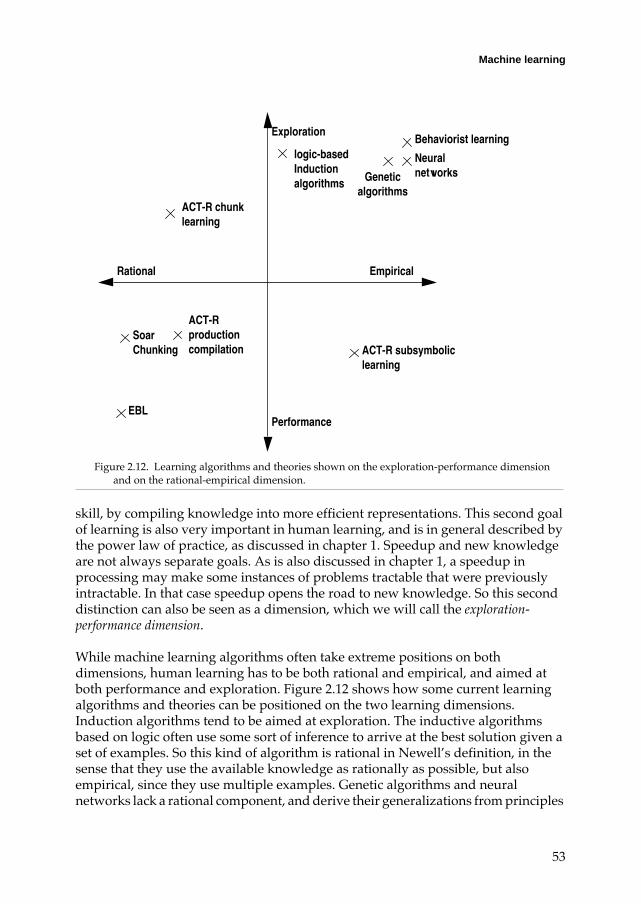
While machine learning algorithms often take extreme positions on both dimensions, human learning has to be both rational and empirical, and aimed at both performance and exploration. Figure 2.12 shows how some current learning algorithms and theories can be positioned on the two learning dimensions. Induction algorithms tend to be aimed at exploration. The inductive algorithms based on logic often use some sort of inference to arrive at the best solution given a set of examples. So this kind of algorithm is rational in NewellÕs definition, in the sense that they use the available knowledge as rationally as possible, but also empirical, since they use multiple examples. Genetic algorithms and neural networks lack a rational component, and derive their generalizations from principles

Soar Chunking

Rational

ACT-R production compilation

Empirical

EBL

ACT-R subsymbolic learning

ACT-R chunk learning

Genetic algorithms

Neural networks

Exploration

Performance

Figure 2.12. Learning algorithms and theories shown on the exploration-performance dimension and on the rational-empirical dimension.

Behaviorist learninglogic-based Induction algorithms


54

inspired by genetics and neuroscience. Behaviorist principles of learning can also be found in this area: they are strictly empirical, and are not interested in performance. This may well be one of the reasons why connectionists are sometimes falsely accused of being a new breed of behaviorists. Analytical algorithms, exemplified by explanation-based learning (EBL), are on the opposite side of the figure. EBL is strictly rational in the sense that all new knowledge is specialized domain knowledge, and is based on a single example. As a consequence it can not gather any new knowledge. SoarÕs chunking mechanism resembles EBL in the sense that learning is based on a single example, summarizing processing in a subgoal, and its stress on rationality.

ACT-RÕs learning mechanisms are harder to classify, since they cannot really be considered as learning algorithms. So their positions in the diagram are approximate. The chunk learning mechanism refers to the fact that ACT-R stores past goals in declarative memory. This may serve several functions. An old goal may just help to increase performance, for example of the fact that three plus four equals seven is memorized as a result of counting it. But a chunk may also contain information gathered from the outside world, or may contain a hypothesis posed by reasoning. If exploration is considered to be a function that proposes a new knowledge element as something that may be potentially useful, the chunk-learning mechanism is more an exploration mechanism than a performance increasing mechanism. Since new chunks are single examples, and are based on reasoning, they are more a product of rational than empirical learning. The empirical aspect of learning is covered by ACT-RÕs subsymbolic learning mechanisms. By examining many examples, ACT-R can estimate the various parameters associated with chunks and productions. But contrary to other subsymbolic learning algorithms, parameter learning is mainly aimed at performance increase. A higher activation allows quicker retrieval of a declarative chunk, and a better estimate of expected-gain parameters allows for more accurate strategy choices. In order to compile a new production in ACT-R, a detailed example must be available in the form of a dependency structure. Although production compilation can be used in any possible fashion, it is not feasible to create large amounts of production rules that contain uncertain knowledge. So the most likely role of production compilation is to increase the efficiency of established knowledge.

Although we have discussed ACT-RÕs mechanisms separately, they usually work in concert. So some new knowledge may initially be learned as a chunk. The parameters of this chunk may be learned by parameter learning. If parameter learning has established that the chunk serves an intermediate function in a problem solving step, it may be transformed into a production rule. So although ACT-RÕs learning mechanisms are not fully fledged learning algorithms, they have the capability, in principle, to cover the whole spectrum of learning means and goals. In later chapters I will show how these primitive learning mechanisms can serve as building blocks for a theory of skill learning.

Conclusions

55

2.5 Conclusions

For the purposes of this thesis, accurate modeling of learning processes in complex problem solving, the ACT-R architecture turns out to be the clear winner with respect to the comparisons made in this chapter. Neural networks Þrst have to solve a number of problems before they can achieve the architecture stadium, and 3CAPS and EPIC do not encompass learning. Although Soar supports learning, it is rigid in the sense that it is mainly aimed at performance increases, and gaining new knowledge is hard to model. SoarÕs theoretical assumptions are the main problem: by deÞning intelligence as using available knowledge, it discounts the importance of gaining new knowledge, and by ignoring performance aspects of behavior it makes detailed predictions of behavior impossible. When the learning mechanisms of ACT-R are examined in the context of machine learning, it turns out that they can in principle cover the whole spectrum of learning.

Although ACT-R is the vehicle I will use in the rest of this thesis, some of SoarÕs ideas will resurface. The idea to key learning to impasses in problem solving is not only rational in the Soar sense, but also, as we will see in chapter 5, in ACT-RÕs.

2.6 Appendix: The ACT-R simulation system

The ACT-R simulation system is a program written in Common Lisp. The basic version is based on a command-line interface in Lisp. Typically, a user loads Common Lisp, loads ACT-R and starts working on a model. A model in ACT-R, which is just a text Þle, usually consists of four areas: global parameter declarations, the contents of declarative memory, the contents of procedural memory and lisp-code to run the particular experiment.

There are two types of declarations for declarative memory: the specification of the chunk types and the initial contents of declarative memory. Although chunk types do not change during the execution of a model, the contents of declarative memory almost always does, since all the goals and subgoals ACT-R creates are added to it. In some models, a specification is added that gives the initial chunks an activation value that differs from the default value 0, for example to reflect that it is a chunk that has been in declarative memory for a long time. The next part of a model is an initial set of production rules. Sometimes initial parameters are specified for these rules. Finally some code is added to run an experiment, and to store results.


56

Figure 2.13 show an example of a very small model, a model that tries to solve an addition-problem. It knows only two addition-facts: 3+4=7 and 4+2=6. Whenever it tries to solve an addition-problem, two rules are applicable: the do-addition rule that tries to retrieve a matching addition-fact and the do-addition-fail rule that give ÒdonÕt knowÓ as an answer. The parameter declaration for the do-addition-fail rule makes sure that its expected gain is lower than the expected gain of the do-addition rule. ACT-R will therefore first try do-addition, and only when that rule fails will do-addition-fail be allowed to fire.

The Lisp code consists of a function that goes through n addition-problems. It generates a random addition-problem, which is given to the model. After one of the

; Very simple ACT-R example model

; Parameter declarations: switch on rational analysis and set Activation Noise to 0.1(sgp :era t :ans 0.1)

; chunk-type declarations(chunk-type addition-problem arg1 arg2 answer)(chunk-type addition-fact addend1 addend2 sum)

; initial contents of declarative memory

(add-dm(fact34

isa addition-factaddend1 3addend2 4sum 7)

(fact42isa addition-factaddend1 4addend2 2sum 6))

; contents of production memory

(p do-addition=goal>

isa addition-problemarg1 =num1arg2 =num2answer nil

=fact>isa addition-factaddend1 =num1addend2 =num2sum =num3

==>=goal>

answer =num3)

(p do-addition-fail=goal>

isa addition-problemanswer nil

==>=goal>

answer dont-know)

; Parameter declaration for do-addition-fail

(spp do-addition-fail :r 0.2)

; Lisp code to run sample experiment

(defun do-it (n)(let ((result 0))

(dotimes (i n)(let ((task (gentemp "goal")))(eval `(add-dm

(,task isa addition-problem arg1 ,(random 5) arg2 ,(random 5))))

(eval `(goal-focus ,task))(run 1)(when

(equal (+ (eval `(chunk-slot-value ,task

arg1))(eval `(chunk-slot-value ,task

arg2)))(eval `(chunk-slot-value ,task

answer)))(setf result (1+ result)))

(pop-goal)))(format t "~%Accuracy = ~6,3F" (/

result n))))

Figure 2.13. Example ACT-R model

Appendix: The ACT-R simulation system

57

production rules has fired, the lisp-function checks whether the answer is correct. After all n problems have or have not been solved, the function gives an accuracy score.

The following trace fragment illustrates the output of the model:

? (do-it 2) Cycle 0 Time 0.000: Do-Addition-Fail Matching latency: 1.000 Action latency: 0.050 Stopped at cycle 1 Run latency: 1.050 Cycle 1 Time 1.050: Do-Addition Matching latency: 0.950 Action latency: 0.050 Stopped at cycle 2 Run latency: 1.000Accuracy = 0.500

Figure 2.14. The ACT-R environment


58

This fragment goes through two addition-problems. The first problem fails, but the second succeeds. The trace shows relatively little detail, but additional tracing options can be used to get more information.

Although ACT-R can be used from a command-line interface, an elaborate environment is also offered. Figure 2.14 shows some of the viewers available in the environment, using the addition example. In the environment, models can be executed step-by-step. At each moment the current contents of declarative and procedural memory can be viewed, as well as the rules that are applicable to the current goal. The environment also provides for a syntax-directed editor that makes it easier for novices to enter chunks and production rules. Finally, the environment supports a tutoring function that can be used in combination with a web-based tutorial. The ACT-R code, as well as the tutorial and the code for the environment, is available from http://act.psy.cmu.edu The models discussed in this thesis are listed in an appendix at the end of the thesis, and are all available from a web page as well.

chapter 2 architectures of cognition · 2016-03-05 · 2: architectures of cognition 28 generally,...

Documents