CHAPTER

2-1

Linear Programming Models: Graphical and

Computer Methods

2

2-2

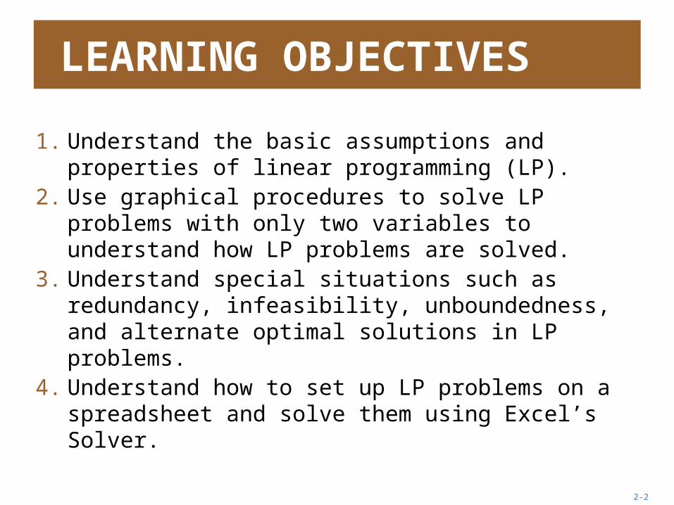
LEARNING OBJECTIVES

1. Understand the basic assumptions and properties of linear programming (LP).

2. Use graphical procedures to solve LP problems with only two variables to understand how LP problems are solved.

3. Understand special situations such as redundancy, infeasibility, unboundedness, and alternate optimal solutions in LP problems.

4. Understand how to set up LP problems on a spreadsheet and solve them using Excel’s Solver.

2-3

Introduction

• Management decisions involve the most effective use of resources

• Most widely used modeling technique is linear programming (LP)

• Deterministic models

2-4

Developing a LP Model

• All LP models can be viewed in terms of the three distinct steps

1. Formulation of simple mathematical expressions

2. Solution to identify an optimal (or best) solution to the model

3. Interpretation of the results and answer “what if?” questions

2-5

Properties of a LP Model

1. Seek to maximize or minimize some quantity (profit or cost)

2. Restrictions or constraints3. Alternative courses of action4. Linear equations or inequalities

(=, ≤, ≥)

2-6

LP Characteristics

• Feasible Region – The set of points that satisfies all constraints

• Corner Point Property – An optimal solution must lie at one or more corner points

• Optimal Solution – The corner point with the best objective function value is optimal

2-7

Formulating a LP Model

• A product mix problem• Decide how much to make of two or more

products

• Objective is to maximize profit

• Limited resources

• Flair Furniture• Best combination of tables and chairs

2-8

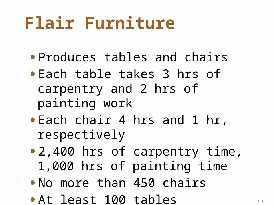
Flair Furniture

• Produces tables and chairs

• Each table takes 3 hrs of carpentry and 2 hrs of painting work

• Each chair 4 hrs and 1 hr, respectively

• 2,400 hrs of carpentry time, 1,000 hrs of painting time

• No more than 450 chairs

• At least 100 tables

• $7 and $5 profit for table and chair

2-9

Decision Variables

• What we are solving for

• Two variables in the Flair problem

• Number of tables (T, Tables or X1)

• Number of chairs (C, Chairs or X2)

• Decision variables can be in different units of measurement

2-10

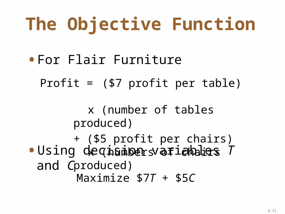
The Objective Function

• States the goal of a problem

• A single objective function

• Objective is often to maximize profit or minimize cost

2-11

The Objective Function

• For Flair Furniture

Profit = ($7 profit per table) x (number of tables

produced)

+ ($5 profit per chairs) x (numbers of chairs

produced)• Using decision variables T and C

Maximize $7T + $5C

2-12

Constraints

• Restrictions or limits on our decisions

• As many as necessary

• Can be independent

• Flair has four constraints• Carpentry time

• Painting time

• Number of chairs to make

• Number of tables to make

2-13

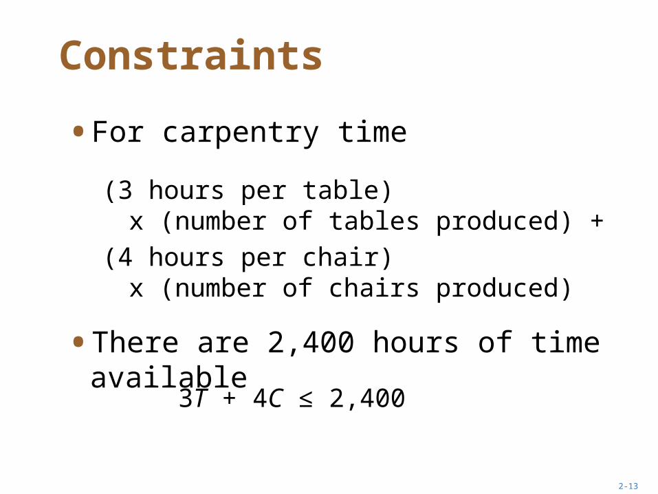
Constraints

• For carpentry time

(3 hours per table) x (number of tables produced) +

(4 hours per chair) x (number of chairs produced)

• There are 2,400 hours of time available

3T + 4C ≤ 2,400

2-14

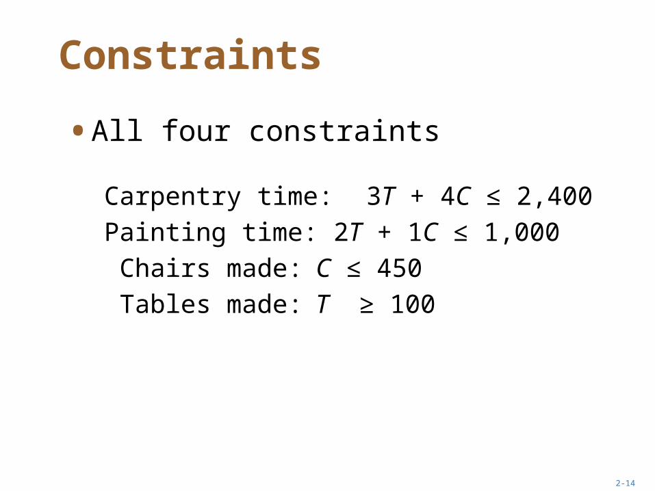
Constraints

• All four constraints

Carpentry time: 3T + 4C ≤ 2,400

Painting time: 2T + 1C ≤ 1,000

Chairs made: C ≤ 450

Tables made: T ≥ 100

2-15

Nonnegativity and Integers

• Decision variables must be ≥ 0, so

• Decision variables may have to be integers

T ≥ 0, and

C ≥ 0

2-16

Flair Model Matrix

TABLES (T) CHAIRS (C) LIMIT

Profit Contribution $7 $5Carpentry 3 hrs 4 hrs 2,400Painting 2 hrs 1 hr 1,000Chairs 0 unit 1 unit 450Tables 1 unit 0 unit 100

2-17

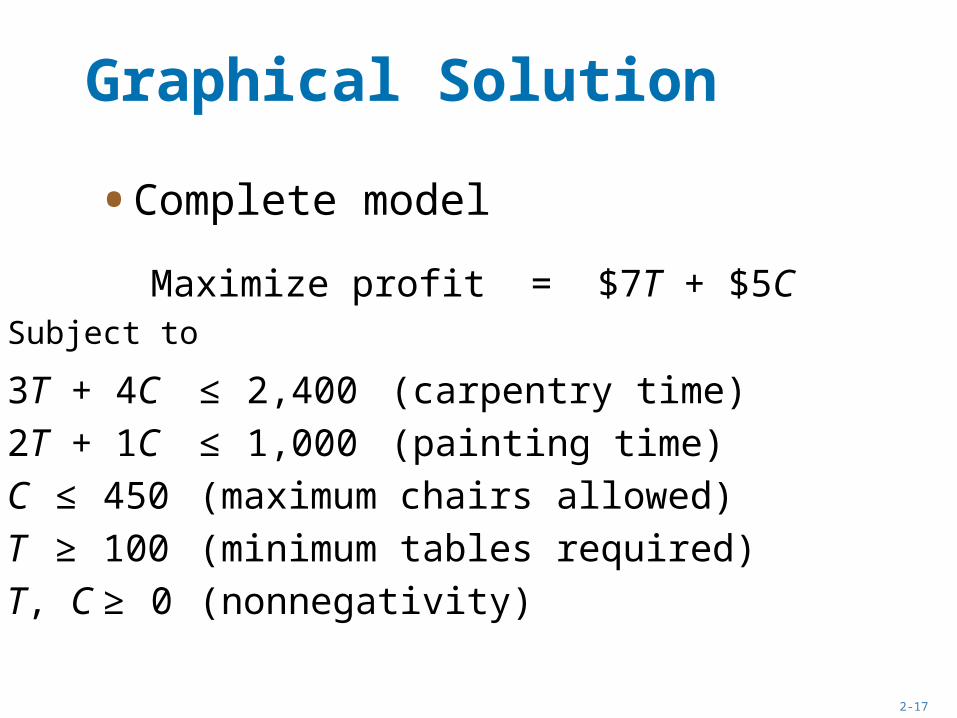
Graphical Solution

• Complete model

Maximize profit = $7T + $5CSubject to

3T + 4C ≤ 2,400(carpentry time)

2T + 1C ≤ 1,000(painting time)

C ≤ 450 (maximum chairs allowed)

T ≥ 100 (minimum tables required)

T, C ≥ 0 (nonnegativity)

2-18

Graphical RepresentationN

umbe

r of

Cha

irs (

C)

Number of Tables(T)

1,000 –

–

800 –

–

600 –

–

400 –

–

200 –

–

0 –| | | | | | | | | | | |

0 200 400 600 800 1,000

(T = 0, C = 600)

(T = 800, C = 0)

Carpentry Constraint Line

Figure 2.1

(T = 400, C = 300)

2-19

Graphical RepresentationN

umbe

r of

Cha

irs (

C)

Number of Tables(T)

1,000 –

–

800 –

–

600 –

–

400 –

–

200 –

–

0 –| | | | | | | | | | | |

0 200 400 600 800 1,000

Figure 2.2

(T = 600, C = 400)

(T = 300, C = 200)

Region Satisfying3T + 4C ≤ 2,400

2-20

Graphical RepresentationN

umbe

r of

Cha

irs (

C)

Number of Tables(T)

1,000 –

–

800 –

–

600 –

–

400 –

–

200 –

–

0 –| | | | | | | | | | | |

0 200 400 600 800 1,000

(T = 0, C = 600)

Carpentry Constraint

Figure 2.3

Painting Constraint

(T = 500, C = 0)

(T = 500, C = 200)

(T = 800, C = 0)

(T = 300, C = 200)

(T = 0, C = 1,000)

(T = 100, C = 700)

2-21

Graphical RepresentationN

umbe

r of

Cha

irs (

C)

Number of Tables(T)

1,000 –

–

800 –

–

600 –

–

400 –

–

200 –

–

0 –| | | | | | | | | | | |

0 200 400 600 800 1,000

Infeasible Solution (T = 50, C = 500)

Figure 2.4

Painting Constraint

Carpentry Constraint

Maximum Chairs Allowed Constraint

Feasible Region

Infeasible Solution(T = 500, C = 200)

(T = 300, C = 200)

Minimum Tables Required Constraint

2-22

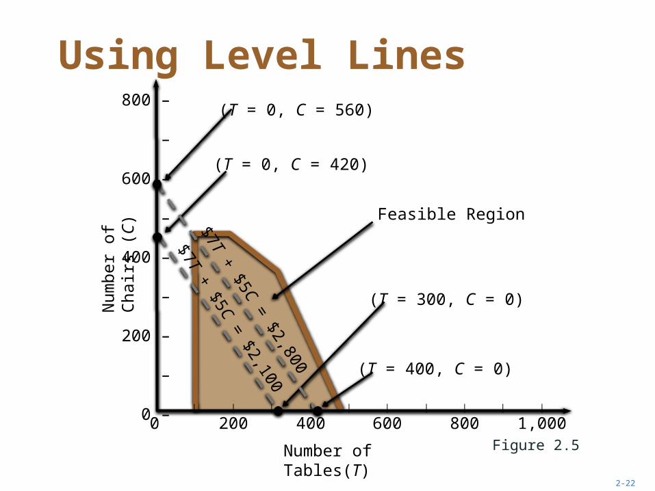
Using Level Lines

Figure 2.5

(T = 0, C = 560)

(T = 400, C = 0)

(T = 300, C = 0)

Feasible Region

(T = 0, C = 420)

$7T + $5C = $2,100

$7T + $5C = $2,800

| | | | | | | | | |

0 200 400 600 800 1,000

800 –

–

600 –

–

400 –

–

200 –

–

0 –

Num

ber

of C

hairs

(C

)

Number of Tables(T)

2-23

1

2 3

4

5

Using Level Lines

Figure 2.6

| | | | | | | | | |

0 200 400 600 800 1,000

800 –

–

600 –

–

400 –

–

200 –

–

0 –

Num

ber

of C

hairs

(C

)

Number of Tables(T)

Painting Constraint

Level Profit Line with No Feasible Points ($7T + $5C = $4,200)

Carpentry Constraint

Optimal Level Profit Line

Optimal Corner Point Solution

$7T + $5C = $2,800

$7T + $5C = $2,100

2-24

Calculating a Solution

• Optimal point 4 is the intersection of two constraints, carpentry and painting

• Solving simultaneously

6T + 8C = 4,800

– (6T + 3C = 3,000)

5C = 1,800

implies C = 360

and T = 320

2-25

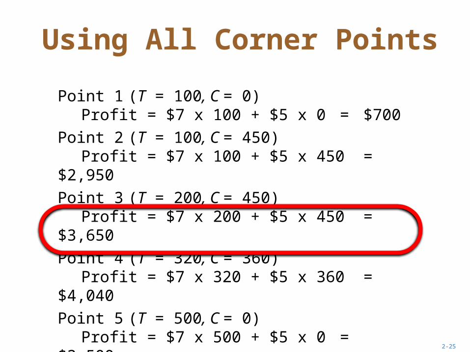
Using All Corner Points

Point 1 (T = 100, C = 0)Profit = $7 x 100 + $5 x 0 = $700

Point 2 (T = 100, C = 450)Profit = $7 x 100 + $5 x 450 =

$2,950

Point 3 (T = 200, C = 450)Profit = $7 x 200 + $5 x 450 =

$3,650

Point 4 (T = 320, C = 360)Profit = $7 x 320 + $5 x 360 =

$4,040

Point 5 (T = 500, C = 0)Profit = $7 x 500 + $5 x 0 = $3,500

2-26

Extension to the Model

Figure 2.7

| | | | | | | | | |

0 200 400 600 800 1,000

800 –

–

600 –

–

400 –

–

200 –

–

0 –

Num

ber

of C

hairs

(C

)

Number of Tables(T)

This Portion of the Original Feasible Region Is No Longer Feasible

($7T + $5C = $2,800)

(T = 300, C = 375) is the New Optimal Corner Point Solution

Optimal Level Profit Line for Revised Problem

1 5

2 3

4

6

7 Additional Constraint C – T ≥ 75 Has a Positive Slope

(T = 320, C = 360) is No Longer Feasible

2-27

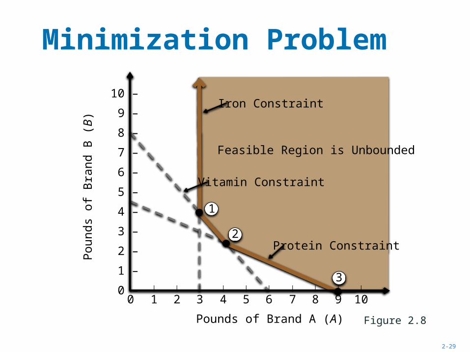
Minimization Problem

• Minimize cost

• Holiday Meal Turkey Ranch• Two types of feed

Minimize cost = $0.10A + $0.15B

subject to

5A + 10B ≥ 45 (protein required)4A + 3B ≥ 24 (vitamin required)0.5A ≥ 1.5 (iron required)A,B ≥ 0 (nonnegativity)

2-28

Minimization Problem

• Data for Holiday Meal Turkey Ranch

Table 2.1

NUTRIENTS PER POUND OF FEED MINIMUM REQUIRED PER TURKEY PER

NUTRIENT BRAND A FEED BRAND B FEED MONTH

Protein (units) 5 10 45Vitamin (units) 4 3 24Iron (units) 0.5 0 1.5Cost Per Pound $0.10 $0.15

2-29

Minimization Problem

Figure 2.8

1

2

3

Feasible Region is Unbounded

Protein Constraint

Iron Constraint

Vitamin Constraint

Pou

nds

of B

rand

B (

B)

Pounds of Brand A (A)

10 –

9 –

8 –

7 –

6 –

5 –

4 –

3 –

2 –

1 –

0 –| | | | | | | | | | |

0 1 2 3 4 5 6 7 8 9 10

2-30

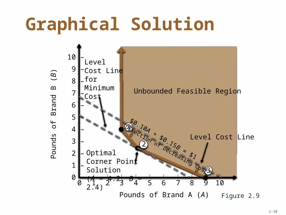
Unbounded Feasible Region

1

2

3

Graphical Solution

Figure 2.9

Pou

nds

of B

rand

B (

B)

Pounds of Brand A (A)

10 –

9 –

8 –

7 –

6 –

5 –

4 –

3 –

2 –

1 –

0 –| | | | | | | | | | |

0 1 2 3 4 5 6 7 8 9 10

Level Cost Line

Level Cost Line for Minimum Cost

Optimal Corner Point Solution(A = 4.2, B = 2.4)

$0.10A + $0.15B = $1

Direction of Decreasing Cost

2-31

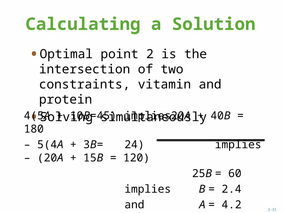
Calculating a Solution

• Optimal point 2 is the intersection of two constraints, vitamin and protein

• Solving simultaneously

4(5A + 10B = 45) implies 20A + 40B = 180

– 5(4A + 3B = 24) implies – (20A + 15B = 120)

25B = 60

implies B = 2.4

and A = 4.2

2-32

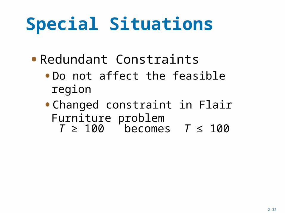
Special Situations

• Redundant Constraints• Do not affect the feasible region

• Changed constraint in Flair Furniture problem

T ≥ 100 becomes T ≤ 100

2-33

Special Situations

C ≤ 450

Figure 2.10

Constraint Changed to T ≤ 100

Carpentry Constraint Is Redundant

Painting Constraint Is Redundant

Fea

sibl

e R

egi

on

Num

ber

of C

hairs

(C

)

Number of Tables(T)

1,000 –

–

800 –

–

600 –

–

400 –

–

200 –

–

0 –| | | | | | | | | | | |

0 200 400 600 800 1,000

2-34

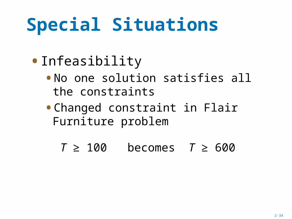
Special Situations

• Infeasibility• No one solution satisfies all the

constraints

• Changed constraint in Flair Furniture problem

T ≥ 100 becomes T ≥ 600

2-35

Region Satisfying Fourth Constraint

Region Satisfying Three Constraints

Special SituationsN

umbe

r of

Cha

irs (

C)

Number of Tables(T)

1,000 –

–

800 –

–

600 –

–

400 –

–

200 –

–

0 –| | | | | | | | | | | |

0 200 400 600 800 1,000

C ≤ 450

Figure 2.11

Constraint Changed to T ≥ 600

2T + C ≤ 1,000

Two Regions Do Not Overlap

3T + 4C ≤ 2,400

2-36

Special Situations

• Alternate Optimal Solutions• More than one solution satisfies all the

constraints

• Changed objective in Flair Furniture problem

$7T + $5C becomes $6T + $3C

2-37

1

2 3

4

5

Feasible Region

Special Situations

Figure 2.12

| | | | | | | | | |

0 200 400 600 800 1,000

800 –

–

600 –

–

400 –

–

200 –

–

0 –

Num

ber

of C

hairs

(C

)

Number of Tables(T)

$6T + $3C = $2,100

Level Profit Line Is Parallel to Painting Constraint

Level Profit Line for Maximum Profit Overlaps Painting Constraint

Optimal Solution Consists of All Points Between Corner Points 4 and 5

2-38

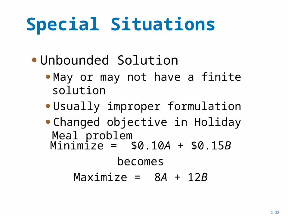
Special Situations

• Unbounded Solution• May or may not have a finite solution

• Usually improper formulation

• Changed objective in Holiday Meal problem

Minimize = $0.10A + $0.15B

becomes

Maximize = 8A + 12B

2-39

UnboundedFeasible Region

Special Situations

Figure 2.13

Pou

nds

of B

rand

B (

B)

Pounds of Brand A (A)

10 –

9 –

8 –

7 –

6 –

5 –

4 –

3 –

2 –

1 –

0 –| | | | | | | | | | |

0 1 2 3 4 5 6 7 8 9 10

Iron Constraint

Protein Constraint

Vitamin Constraint

8A + 12B = 1008A + 12B = 80

Direction of Increasing Value

Value Can Be Increased to Infinity

2-40

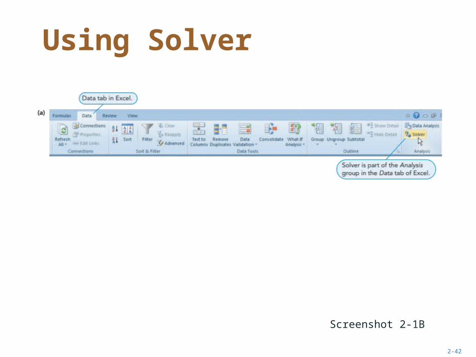
Using Excel’s Solver

• Excel’s built-in LP solution tool for LP

• Commonly available and easy access

• Familiar software

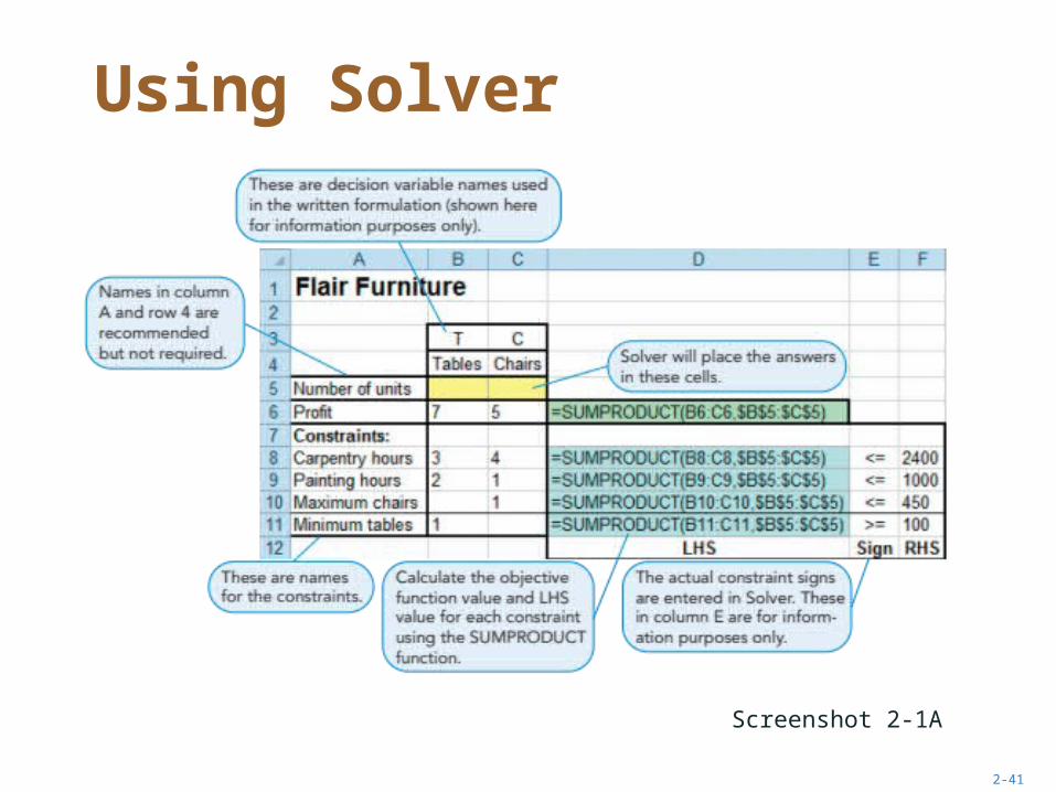
2-41

Using Solver

Screenshot 2-1A

2-42

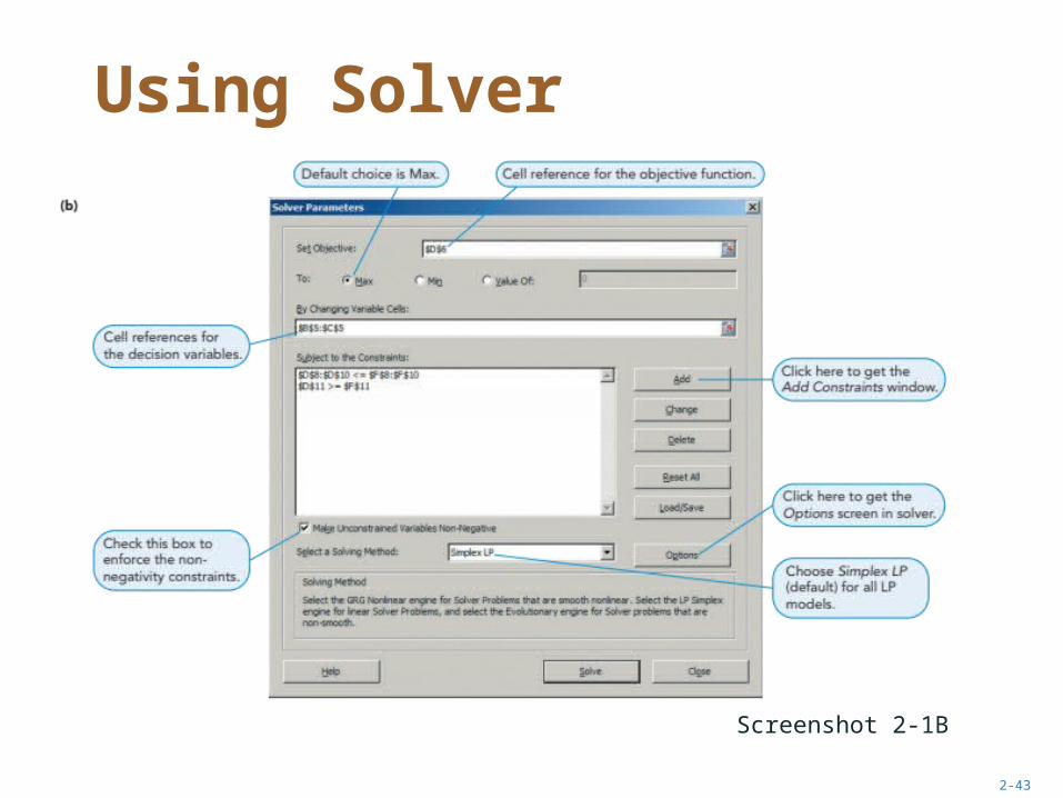
Using Solver

Screenshot 2-1B

2-43

Using Solver

Screenshot 2-1B

2-44

Using Solver

Screenshot 2-1C

2-45

Using Solver

Screenshot 2-1D

2-46

Using Solver

Screenshot 2-1E

2-47

Using Solver

Screenshot 2-1F

2-48

Using Solver

Screenshot 2-2

2-49

Using Solver

Screenshot 2-3A

2-50

Using Solver

Screenshot 2-3B