1

Chapter 17

Gene predictions and annotations

Roderic Guigó (Insitut Municipal d’Investigació Mèdica, Centre de Regulació Genòmica, Universitat Pompeu Fabra, Barcelona, Spain)

and Michael Q. Zhang M.Q. (Cold Spring Harbor Laboratory, NY, USA)

Table of contents 1. Introduction 2. Ab initio gene prediction a. Prediction of signals b. Prediction of exons c. Exon assembly into genes d. Gene Prediction Programs 3. Comparative gene prediction

a. Genomic Query against Protein or cDNA Target b. Genomic Query against Genomic Target c. Prediction of Selenoproteins

4. Accuracy of gene predictions a. Measures of Prediction Accuracy b. Accuracy in single gen sequences c. Accuracy in Large Genomic Sequences

5. Genome annotation systems References 1. INTRODUCTION After the genome of an organism is sequenced and assembled, comprehensive and accurate initial gene prediction and annotation by computational analysis have become the necessary first step towards understanding of the functional content of the genome. This chapter describes typical computational methods for identification of protein coding genes in a mammalian genome. The organization of a gene, as any other biological structure, is determined by functional and evolutionary constraints; all computational methods are therefore based on our experimental understanding of such constraints. Similar structure features would imply similar function and a tendency to be conserved through evolution. According to the central dogma, genetic information flows as DNA → RNA → Protein (see Chapters 5 and 6). Namely, a gene is first transcribed into a pre-mRNA, this transcript is subsequently processed (i.e. capped, spliced and polyadenylated) and the mature mRNA transcript is then transported from the nucleus into the cytoplasm for translation into the gene product – a functional protein. An example of a eukaryotic gene structure and its corresponding mature mRNA transcript are depicted in Figure 17.1. There are two types of genetic elements with respect to primary structure of proteins: short cis-regulatory elements (also called “signals”, mostly in non-coding regions) that control how the gene is

2

expressed, and coding sequences (CDSs) that code for the gene product (protein). There are also RNA genes such as miRNAs and tRNAs, , but they are not the focus of this chapter. Since the majority of the mammalian genes have introns, the key in gene prediction is to detect splice site signals and to locate CDSs. In the early 80s, computer methods were developed to find genes either by detecting extended CDS regions based on codon usage (Staden & McLachlan 1982) or coding periodicity (Fickett 1982), or by detecting splicing signals (Mount 1982, Staden 1984). Later, more complex algorithms based on modern statistical (e.g. linear or quadratic discriminant analysis, or LDA/QDA), linguistic (e.g. Hidden Markov Model or HMM) or machine-learning (e.g. Artificial Neural Networks or ANN) techniques have been developed to combine various sequence features for more accurate gene predictions. As more genomes become available, comparative genomics can offer even better prediction than ab initio methods for homologous genes. Although gene prediction tools have become more sophisticated, prediction accuracy is still far from satisfactory. Up to now, the total number of human genes, ranging from 24,500 to 45,000 (Pennisi 2003), still cannot be estimated with certainty, and current mammalian gene counts are highly hypothetical in nature. There is still a long way to go before gene prediction programs can produce accurate predictions of the gene content in mammalian genomes. 2. AB INITIO GENE PREDICTION As most mammalian genes contain introns, here we mainly describe some basic methods for predicting coding exons of the intron containing genes (see Zhang 2002 for review and discussion of more general types of exons and their predictions).

a. Prediction of signals

There are four basic signals for any coding exon predictions: the translational start site (the START site), the 5’ splice site (5’ss, or donor site), the 3’ splice site (3’ss, or acceptor site), the branch site and the translational stop site (the STOP codon). The simplest measure for a signal site is so-called consensus (word pattern). For example, a STOP site may be any of TAA, TAG or TGA (the ratio among these three stop codons in mammalian genomes is about 1:1:2). The ATG site and the START site may be characterized by the Kozak consensus GCCGCCRCCATGG (Kozak 1987). Splice site consensus was first catalogued by Mount (1982) and later was refined with more data by Senapathy et al. (1990): donor site AG|GTRAGT, acceptor site (Y)nNCAG|G and branch site CTRAY (the average distance between the branch point “A” to the 3’ss boundary, indicated by “|” in the acceptor site) is 26 bases. Senapathy et al. actually presented the splice signals by more quantitative frequency matrices (see table 17.1), where each matrix element Mij is equal to the frequency count of the base “i” at position “j” from the training set of aligned splice site sequences. If one defines fij = Mij/100, and fi as the background frequency of nucleotide i, then the popular log-odd scoring matrix (weight matrix model, or WMM) Sij = log(fij / fi) scores the signal as the sum of the scores over the bases within the signal.

3

Although useful in many cases, there are at least two main problems with any WMM approache. Firstly, it assumes that bases at different positions are independent. There are many ways to incorporate base dependencies. One method is to assume that each base is correlated with its neighboring bases (so-called Markov dependence or weight array model, WAM, Zhang 1993). It is equivalent to extending the rows to doublets (Markov order-1: AA, AC AG, etc.) or to triplets (Markov order-2: AAA, AAC, AAG, etc.). But more dependencies result in more parameters to be estimated and it requires much more training data. Another method is to apply a decision tree (so-called Maximum Dependence Decomposition, MDM, Burge & Karlin 1997) to partition total training data into subsets so that splice site bases within each subset are approximately independent and hence can be modeled by a separate WMM. This also ignores the GC-content of the gene locus. It is well known that a mammalian genome has large variations in GC-content, often referred to as isochores (Bernardi 1995), therefore all signal compositions will be highly biased by the GC-content. More modern gene prediction tools use GC-content specific signal models (Zhang 1998). For example, the GC-specific splice site WMMs are shown in table 17.2 with each element representing the frequency count obtained from both “low” and ”high” GC genes (Zhang 1998). There are other ways one may further improve the accuracy of a signal prediction. For instance, one could model secondary structures of pre-mRNAs (e.g. Patterson et al. 2002). But the most effective way of improving signal site prediction is to combine flanking sequence features (for example, a donor score can be combined with upstream exon and down stream intron scores by LDA, Solovyev et al. 1994). Here we have only described statistical methods; there are also several machine-learning methods (e.g. Lapedes et al. 1990, Degroeve et al 2002) in parallel to each of the statistical approaches. Recently, Pertea et al (2001) compared several leading prediction programs: NetGene2 (Brunak et al. 1991, http://genome.cbs.dtu.dk/services/NetGene2/), HSPL (Solovyev et al. 1984, http://genomic.sanger.ac.uk/), NNSplice (Reese MG et al. 1997, http://www.fruitfly.org/seq_tools/splice.html) GENIO (Mache & Levi, 1998, http://genio.informatik.uni-stuttgart.de/GENIO/splice/) and SpliceView (Rogozin & Milanesi, 1997, http://l25.itba.mi.cnr.it/~webgene/wwwspliceview.html) with their own GeneSplicer (Pertea et al., 2001, http://www.tigr.org/tdb/GeneSplicer/gene_spl.html), and concluded that “Overall, NetGene2 appears to be the best for donor site prediction, while for acceptor sites either GeneSplicer, NetGene2 or HSPL perform comparably. One advantage of GeneSplicer for the latter task is that its thresholds can be adjusted by the user to vary the false negative and false positive rates”. The best average of error (false-positive + false-negative) rate for either donor or acceptor site prediction is about 5%. This may sound not bad if the search is restricted in a short (say, coding) region. If one uses any predictor to search a large region of a genome, the false-positive rate is unacceptable because for every true site there are hundreds of pseudo-sites. For example, if a large region has 40 true sites and 4000 pseudo-sites, one true site would be missed (2.5% false-negatives) and 100 pseudo-sites would be predicted as true sites (2.5% false-positives)! Since adjacent donor site and acceptor site are not independent (Zhang 1998), this correlation can be explored for further eliminating false-positives. For short introns, occurring mostly in lower eukaryotes, an intron is recognized by the interaction of splicing

4

factors binding across the intron-ends (hence 5’ss – 3’ss correlation, Lim & Burge 2001). In vertebrates, exons are much shorter, recognition of exons by the interaction of splicing factors binding across the exon-ends (hence 3’ss – 5’ss correlation, Zhang 1998) is the key (Robbertson et al. 1990). Therefore mammalian functional splice sites can only be effectively identified simultaneously through exon recognition. An additional complication, dealt poorly with by current splice site prediction programs is the presence of non-canonical sites. At least 1% of all introns do not conform to the canonical AG-GT boundaries (Burset et al., 2000), and they are systematicall ignored by splice site and gene prediction methods.

b. Prediction of exons In addition to signal features, prediction of exons (here we only discuss internal coding exons which can be easily generalized to other types of exons. See Zhang 1998 for the complete classification of 12 types of exons in the mammalian genomes) should also require content features for both exon regions and flanking intron regions (typically < 100 bp on each side). To discriminate CDS from introns, the best content feature is the frame-specific hexamer frequency score, named so because it captures codon-bias information and codon-codon correlation (Fickett & Tung 1992, Guigó, 1998). There are many ways to construct such a score, both Log-Odd score LE(w,i) = log [ fE(w,i) / fI(w) ] and preference score PE(w,i) = fE(w,i) / [fE(w,i) + fI(w)] are popular among exon finders, where fE(w,i) is the frequency of hexamer w in frame i calculated from known exon training data and fI(w) is the frequency of w calculated from known flanking introns. If the hexamer w is more likely to be found in an exon at the given frame than in an intron, LE will be positive (PE will be greater than 1/2). PE is easier to use as it ranges from 0 to 1, and has been used in both LDA (HEXON: Solovyev et al. 1994) and QDA (MZEF: Zhang 1997) exon finders. In addition to coding measures, exon size is another important feature variable one must consider. For human internal coding exons, the size distribution is close to a log-normal distribution centered around 125 bp (Zhang 1998). For intron regions, one may also construct similar hexamer scores: LI(w) = log [ fI(w) / fE(w)] = −LE(w) or PI(w) = fI(w) / [fE(w) + fI(w)] = 1 – PE(w), where fE(w) is the average of fE(w,i) over all three reading frames (i.e. fE(w) = [fE(w,0) + fE(w,1) + fE(w,2)]/3). These coding measures can only help with prediction of CDS regions, there has not been any effective method for predicting non-translated regions (UTRs) of an exon. With a training set of exons and pseudo-exons (randomly selected AG-ORF-GT regions, also called a spliceable open reading frame, i.e. open reading frames bounded by the conserved 3’ss AG and 5’ss GT pair) and a set of feature variables x = (x1, x2, …,xK) (for example, x1 = 5’-flanking intron region score = average LI(w) over all hexamers in the 5’-flanking intron region, x2 = acceptor site score, x3 = maximum exon score = average LE(w,i) over all hexamers in reading frame i and then take the maximum over i, x4 = exon size, x5 = donor site score, x6 = 3’-flanking intron region score, etc.), each training sample (a true exon or a pseudo-exon) can be represented by a point in the k-dimensional feature space. There are many statistical or machine-learning methods (most of them have been tried) that can be used to build an optimal (in the sense of minimization of false-positive and false-

5

negative errors using cross-validation tests) discrimination function. This function is a decision surface (exon predictor) in the k-dimensional feature space that can best separate true exons from pseudo-exons. In MZEF (Zhang 1997), QDA is implemented. Namely, the two training sample points (true exons and pseudo-exons) in the feature space are approximated by two separate k-dimensional Gaussian distributions characterized by the sample means and covariance matrices (estimated from the training data), the intersection of the two Gaussian distributions is a (k-1)-dimensional quadratic discrimination surface separating the two sample points in an optimal way (for a pedagogical introduction on DNA pattern discrimination, see Zhang 2000). When the two Gaussians are assumed to have the same covariance matrix, the surface will become a hyper-plane and QDA will reduce to LDA, a method implemented in HEXON (Solovyev et al. 1994) that is the exon-finder part of FGENEH (see below). Internal coding exon finding performance (Zhang 1997) is shown in table 17.3 using a dataset of 570 mammalian single-gene sequences (Burset & Guigo 1996, see section 4).

Splice site identification helps exon recognition, internal coding exon measure can help further improve functional splice site selection. Indeed, Thanaraj and Robinson (2000) found that (i) a high proportion of false positive splice sites from computational predictions occur in the vicinity of real splice sites; and (ii) current algorithms are misled to predict wrong splice sites more often when the coding potential ends within +/-25 nucleotides from real sites than when it ends at father positions. Their integrated system (MZEF-SPC) with Splice ProximalCheck (SPC) as a front-end filter for MZEF was able to eliminate 2/3 of the predicted false positives at the expense of loosing 1/10 of predicted true positives. In fact, these “false positive” splice sites could be alternate splice sites in a lot of cases. Exon extensions and truncations are commonly seen when an exon is skipped. Existing alternative exons obviously makes it so much harder to predict accurately the splice sites, as there are quite a number of real splice sites. Over half of all genes are alternatively spliced, and over 10 isoforms on average per gene, so the in-silico “false positives” may actually be “false negatives” in-vitro!

c. Exon assembly into genes As exons are not independent, by splicing exons together to assemble a gene one can further eliminate false exon predictions by imposing translatability (i.e. adjacent exons must maintain the open reading frame). The main difficulty in exon assembly is the combinatorial explosion problem: the number of ways N candidate exons may be combined grows exponentially with N. The key idea of computational feasibility comes from dynamic programming (DP), which allows finding “optimal assembly” quickly without having to enumerate all possibilities (Gelfand and Roytberg 1993). DP is also used in GeneParse (Snyder & Stormo 1993) to recursively search for exon-intron boundaries with signal and content measures obtained by a neural network. The FGENEH (Solovyev et al. 1995) algorithm incorporate 5’-, internal, and 3’-exon identification linear discriminant functions and a dynamic programming approach for exon assembly. A more efficient dynamic programming algorithm was introduced by Guigó (1998), and it is incorporated in the program GENEID (Guigo et al., 1992, Parra et al., 2000).

6

A novel advance in gene prediction methodologies was the application of generalized Hidden Markov Models (HMMs) initially implemented in the Genie algorithm (Kulp et al. 1996, HMM was first used in a bacterial gene finder by Krogh et al. 1994 after its success in protein modeling). Soon after, it was implemented in the Genscan algorithm (Burge & Karlin 1997) to predict multiple genes. Several other HMM-based gene prediction programs were developed later: VEIL (Henderson et al 1997), HMMGENE (Krogh 1997) and FGENESH (Salamov & Solovyev 2000). In a HMM approach, different types of structure components (such as, exon or intron) are characterized by a state, a gene model is thought to be generated by a state machine: starting from 5’ to 3’, each base-pair is generated by a “emission probability” conditioned on the current state and surrounding sequences and transition from one state to another is governed by a “transition probability” which obeys all the constraints (such as an intron can only follow an exon, reading frames of two adjacent exons must be compatible, etc.). All the parameters of the “emission probabilities” and the (Markov) “transition probabilities” are learned (pre-computed) from some training data. Since the states are unknown (“Hidden”), an efficient algorithm (called the Viterbi algorithm, similar to DP) may be used to select a best set of consecutive states (called a “parse”), which has the highest overall probability compared with any other possible parse of the given genomic sequence (see Rabiner 1989 for a tutorial on HMMs). The reason these fully probabilistic state models have become preferable is that all scores are probabilities themselves and the weighting problem has become a matter of counting relative observed state frequency. It is easy to add more states (such as intergenic regions, promoters, UTRs, etc.) and transitions into HMM-based models to allow partial genes, intronless genes, even multiple genes or genes on different strands to be incorporated. These features are essential when annotating genomes or large contigs in an automated fashion. The advantage of modeling both strands simultaneously is that it avoids the prediction of overlapping genes on the two strands, which presumably are very rare in mammalian genomes, although in some cases, they may a natural regulatory function.

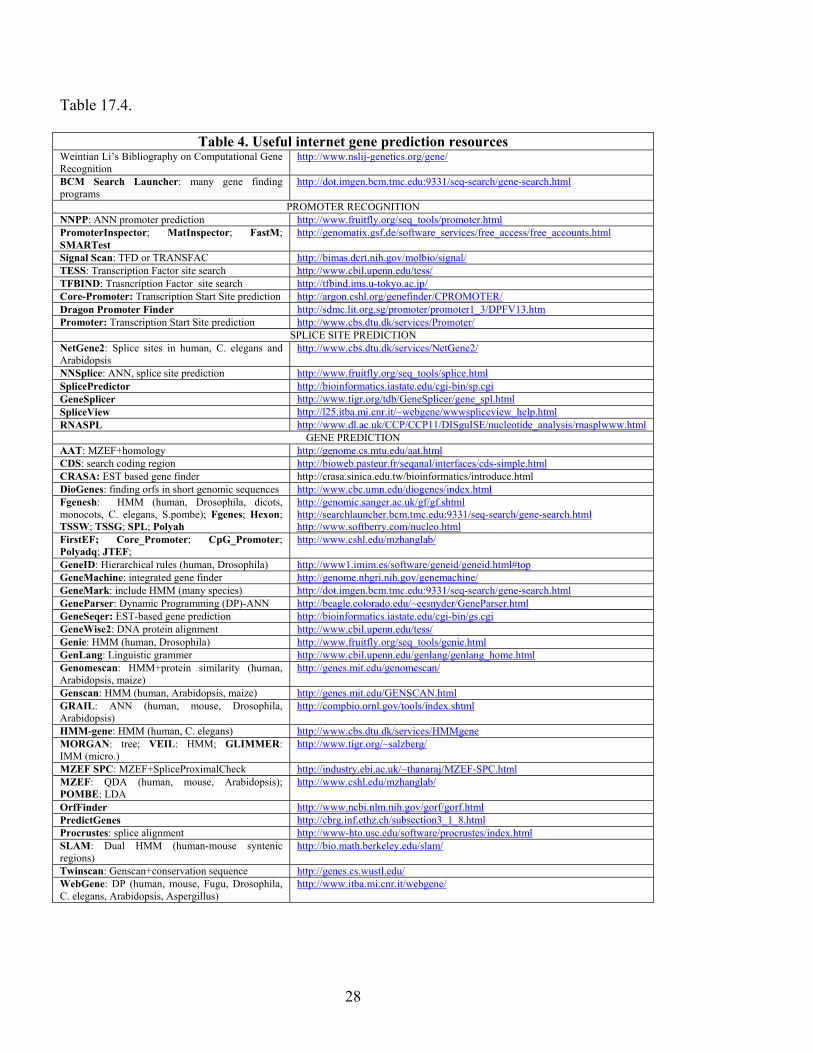
d. Gene prediction programs In table 17.4, we have listed a number of the most popular gene finders available on the internet, as well as other useful gene prediction resources. Benchmarks on the accuracy of these programs are described in section 4. It has been reported that by integrating different programs together, one could achieve higher accuracy. For example, in DIGIT (Yada et al, 2003), a Bayesian procedure and a HMM were used to combine the results of FGENESH, GENSCAN and HMMGENE to report better performance than the individual programs (see section 4). 3. COMPARATIVE GENE PREDICTION The rationale behind comparative or similarity base gene prediction methods is that the regions in the genome sequence coding for proteins are generally more conserved during evolution that non-functional regions (figure 17.2). Essentially, there are two main classes of similarity based approaches for gene identification: the comparison of the DNA query sequence with a protein or cDNA sequence, or a database of such sequences, and the

7

comparison of two or more genomic sequences. In both approaches query and target sequences may be from the same or different species.

a. Genomic Query Against Protein or cDNA Target

The backbone of similarity-aided or similarity-based gene structure determination is constituted by those methods that rely on a comparison of the query sequence with protein, or cDNA sequences. Although mostly known as a database search program, BLASTX (Altschul et al., 1990; Gish and States, 1993) illustrates the rationale behind this approach. With BLASTX a genomic query is translated into a set of amino acid sequences in the six possible frames and compared against a database of known protein sequences. The assumption is that those segments in the genomic query similar to database proteins are likely to correspond to coding exons. A similar assumption is behind the comparison of the genomic query against a database of cDNA sequences (such as ESTs), using BLASTN (Altschul et al., 1990), FASTA (Pearson, 1999), or similar programs. Such database search programs, however, are not dedicated gene prediction tools; they report exclusively matching sequences, but are not capable of automatically identifying start and stop codons or splice sites. Thus, after a database search and the identification of potential targets, additional tools are required to define exonic structures. One approach is to use the top database match as target sequence, and obtain a so-called spliced alignment between this and the genomic query. In such an alignment, large gaps - likely to correspond to introns - are only allowed at legal splice junctions. A popular program (SIM4) to calculate such a spliced pairwise alignment has been developed by Florea et al. (1998). One of the first programs for the specific task to map ESTs onto a genomic sequence is EST_GENOME (Mott, 1997). Splicing alignment algorithms with protein targets require a conceptual translation of the query sequence, computation of the alignment and post-processing, which includes the combinatorial problem of finding the best fit of a multi-exon structure to a related protein. Most such splicing alignment tools employ for this task dynamic programming techniques. Therefore, gene prediction in large scale sequences may become extremely time- and space-demanding. This investment, however, is usually at the benefit of prediction accuracy. PROCRUSTES (Gelfand et al., 1996) and GENEWISE (Birney and Durbin, 1997) are powerful programs to predict genes based on a comparison of a genomic query with protein targets. GENEWISE is at the core of the ENSEMBL system (see Section 5). GENESEQER (Usuka and Brendel, 2000) is a similar spliced alignment program for plant genomes. In an alternative approach, the results of a database search can be integrated in a more or less ad-hoc way into the framework of a typical ab initio gene prediction program. In essence, these methods promote candidate exons in the query sequence for which similar known coding sequences exist. Indeed, the score of the candidate exon - initially a function of the score of the splice (start, stop) sites and of the coding potential of the exon sequence (see Section 2)- is increased as a function of the similarity between the candidate exon and

8

the known coding sequences. In this way, candidate exons showing similarity to known coding sequences, are more likely to be included in the final gene prediction. In theory, this approach should produce predictions as accurate as pure ab initio programs when no similar target sequences exist, but more accurate ones (ideally, as accurate as those from splicing alignment tools) when such target sequences do exist. One popular example of this approach is the program GENOMESCAN (Yeh et al., 2001), an extension of GENSCAN over which it reports increased accuracy. CRASA (Chuang et al., 2003) is a recently developed method that uses ESTs instead.

b. Genomic Query Against Genomic Target

With availability of genome sequences for an increasing number of eukaryote organisms, whole genome sequence comparisons are gaining popularity as a means of identifying protein coding genes. Under the assumption that regions conserved in the sequence will tend to correspond to coding exons from homologous genes, a number of programs have been recently developed.. The program EXOFISH (Crollius et al., 2000) was one of the first such programs developed and predicts human exons based on a comparison with a database of random sequences from Tetraodon nigroviridis, a puffer fish species. Latter developments followed notably different approaches.

In one such approach (Pedersen and Scharl, 2002; Blayo et al., 2002), the problem is stated as a generalization of pairwise sequence alignment: given two genomic sequences coding for homologous genes, the goal is to obtain the predicted exonic structure in each sequence maximizing the score of the alignment of the resulting amino acid sequences. Both, Blayo et al. (2002) and Pedersen and Scharl (2002) solve the problem through a complex extension of the classical dynamic programming algorithm for sequence alignment.

In a different approach, the programs SLAM (Pachter et al., 2002, http://baboon.math.berkeley.edu/~syntenic/slam.html) and DOUBLESCAN (Meyer and Durbin, 2002) combine sequence alignment Pair Hidden Markov Models (HMMs), (Durbin et al., 1998), with gene prediction Generalized HMMs (GHMMs; Burge and Karlin, 1997) into the so-called Generalized Pair HMMs. In these, gene prediction is not the result of the sequence alignment, as in the programs above, but both gene prediction and sequence alignment are obtained simultaneously.

A third class of programs adopt a more heuristic approach, and clearly separate gene prediction from sequence alignment. The programs ROSETTA (Batzoglou et al., 2000), SGP1 (from Syntenic Gene Prediction, Wiehe et al., 2001, http://195.37.47.237/sgp-1/), and CEM (from the Conserved Exon Method, Bafna and Huson, 2000) are representative of this approach. All these programs start by aligning two syntenic sequences and then predict gene structures in which the exons are compatible with the alignment.

Although similarity based gene prediction with homologous genomic sequences may produce high quality results (Miller, 2001), an obvious shortcoming is the need for two homologous sequences. Also, genes without a homolog in the partner sequence will escape detection. This is particular problematic if species are compared where gene order or

9

synteny is not preserved. Given only a single query sequence, it is therefore desirable to automatically search for homologous sequences or syntenic chromosome stretches in other species that are suited to be applied to similarity based programs. The programs TWINSCAN (Korf et al., 2001, http://genes.cs.wustl.edu/query.html/ ) and SGP2 (Parra et al., 2003, http://genome.imim.es/software/sgp2/ ) attempt to address this limitation. The approach in these programs is reminiscent of that used in GENOMESCAN (Yeh et al., 2001) to incorporate similarity to known proteins to modify the GENSCAN scoring schema. Essentially, the query sequence from the target genome is compared against a collection of sequences from the informant genome (which can be a single homologous sequence to the query sequence, a whole assembled genome, or a collection of shotgun reads), and the results of the comparison are used to modify the scores of the exons produced by "ab initio'' gene prediction programs. In TWINSCAN, the genome sequences are compared using BLASTN and the results serve to modify the underlying probability of the potential exons predicted by GENSCAN. In SGP2, the genome sequences are compared using TBLASTX (Gish, W., 1996-2002, http://blast.wustl.edu ), and the results used to modify the scores of the potential scores predicted by GENEID.

TWINSCAN, SGP2, and SLAM have been successfully applied to the annotation of the mouse genome (Mouse Genome Sequence Consortium, 2002), and have helped to identify previously unconfirmed genes (Guigó et al., 2003). Up to date predictions of these programs on the human and rodent genomes can be accessed through the UCSC genome browser and the ENSEMBL system (see section 5).

c. prediction of selenoproteins The characterization of eukaryotic selenoproteins illustrates nicely the power of comparative gene prediction methods. In selenoproteins, the codon TGA is translated into a selenocysteine residue. Identification of transcript encoding selenocysteine-containing proteins is particularly difficult even if the full-length cDNA of the gene is known, because computational gene prediction programs—including simple ORF finders—assume without exception that the TGA triplet codes for stop codon. The alternative decoding of this codon is due to an mRNA structure, the SEleno Cysteine Insertion Element Sequence (SECIS), located at the 3' UTR of the selenoprotein-encoding genes. However, there is very little sequence conservation in the SECIS element, and searching for potential SECIS structures in eukaryotic genomes produces an overwhelming number of false positive hits. Castellano et al. (2001) developed a computational method to identify selenoproteins-encoding genes, which relies on the concerted prediction of SECIS structures and genes with in-frame TGA codons. In this regard, the fact that the region between the in-frame TGA codon and the real stop codon in selenoprotein genes exhibits the codon bias characteristic of protein coding regions is of advantage to selenoprotein gene prediction. This approach lead to the identification of the three selenoproteins so far identified in the Drosophila genome (Castellano et al., 2001). When applied to mammalian genomes with lower coding density, however, the approach was less successful. In this regard, the availability of different mammalian and vertebrate genomes is essential for the characterization of mammalian selenoproteins. Comparative analysis helps in the identification of selenoproteins, primarily, at two different levels: 1) SECIS sequences are characteristically conserved

10

between orthologous genes of species at the appropriate phylogenetic distance; and 2) coding sequence conservation across a UGA codon between a query and a target DNA sequence may strongly suggest a Sec coding function (see Figure 17.4). In contrast, if the conservation vanishes downstream of the UGA codon, this is often indicative of a stop codon function.

Conservation of SECIS sequences between human and mouse orthologous selenoproteins has been used in the search for mammalian selenoproteins (Kryukov et al. 2003), while conservation of UGA-flanking sequences as an indication of Sec coding function has been used in the comparative analysis of the human and fugu genomes (Castellano et al., in press). Indeed, sequence comparisons of TGA interrupted predicted genes obtained independently in these two genomes has lead to the identification of SelU, a novel selenoprotein family (see Figure 17.3). 4. ACCURACY OF GENE PREDICTIONS One the first comprehensive comparative analysis of gene prediction programs was published by Burset and Guigó (1996), where a number of performance metrics were introduced to evaluate the accuracy of gene predictions. We describe first these measures, and discuss a few of the more important benchmarks concerning accuracy of gene predictions in mammalian genomes. For a more detailed discussion and critical reviews of measures of gene prediction accuracy, see the papers by Bajic (2000) and Baldi et al. (2000). An extensive review on the accuracy of gene finding programs can be found in Guigó and Wiehe (2003).

a. Measures of Prediction Accuracy

To evaluate the accuracy of a gene prediction program on a test sequence, the gene structure predicted by the program is compared with the actual gene structure of the sequence. The accuracy can be evaluated at different levels of resolution. Typically, these are the nucleotide, exon, and gene levels. These three levels offer complementary views of the accuracy of the program. At each level, there are two basic measures: Sensitivity and Specificity, which essentially measure prediction errors of the first and second kind. Briefly, Sensitivity is the proportion of real elements (coding nucleotides, exons or genes) that have been correctly predicted, while Specificity is the proportion of predicted elements that are correct. More specifically, if TP are the total number of coding elements correctly predicted, TN, the number of correctly predicted non-coding elements, FP the number of non-coding elements predicted coding, and FN the number of coding elements predicted non-coding, then, in the gene finding literature, Sensitivity is defined as Sn=TP/(TP+FN) and Specificity as Sp=TP/(TP+FP).Both, sensitivity and specificity, take values from 0 to 1, with perfect prediction when both measures are equal to 1. Neither Sn nor Sp alone constitute good measures of global accuracy, since one can have high sensitivity with little specificity and vice versa. It is desirable to use a single scalar value to summarize both of them. In the gene finding literature, the preferred such measure on the nucleotide level is the correlation coefficient defined as

11

( ) ( )

( ) ( ) ( ) )( FNTNFPTPFPTNFNTPFPFNTNTPCC +×+×+×+

×−×=

CC ranges from -1 to 1, with 1 corresponding to a perfect prediction, and -1 to a prediction in which each coding nucleotide is predicted as non-coding and vice versa. At the exon level, an exon is considered correctly predicted only if the predicted exon is identical to the true one, in particular both 5' and 3' exon boundaries have to be correct. A predicted exon is considered wrong (WE), if it has no overlap with any real exon, and a real exon is considered missed (ME) if it has no overlap with a predicted exon. A summary measure on the exon level is simply the average of sensitivity and specificity. At the gene level, a gene is correctly predicted if all of the coding exons are identified, every intron-exon boundary is correct, and all of the exons are included in the proper gene.

b. Accuracy in single gene sequences Table 17.5 reproduces the results from the benchmark by Burset and Guigó (1996). These authors evaluated seven programs in a set of 570 vertebrate single gene genomic sequences deposited in GenBank after January 1993. This was done to minimize the overlap between this test set and the sets of sequences which the programs had been trained on. Average CC for the programs analyzed ranged from 0.65 to 0.78 at the nucleotide level, while the average exon prediction accuracy ((Sn+Sp)/2) ranged from 0.37 to 0.64. It can not be ruled out, however, that some of the exons considered mispredicted, may actually correspond to yet to be discovered splice isoforms of the gene Rogic et al. (2001) published recently a new independent comparative analysis of seven gene prediction programs. The programs were again tested in single gene sequences from human and rodent species. In order to avoid overlap with the training sets of the programs, only sequences were selected that had been entered in GenBank, after the programs were developed and trained. Table 7.6 shows the accuracy measures averaged over the set of sequences effectively analyzed for each of the tested programs. The programs tested by Rogic et al. (2001) showed substantially higher accuracy than the programs tested by Burset and Guigó (1996): average CC at the nucleotide level ranged from 0.66 to 0.91, while average exon prediction accuracy ranged from 0.43 to 0.76. Interestingly, DIGIT, a program that integrates the output of several gene finders, reports the Rogic et al. dataset gave a sensitivity of 0.80, and a specificity of 0.84, which is substantially larger than that of any individual program. [However, one needs to be cautious when optimizing the performance of a gene prediction program or system in one particular sequence data set, since this may lead to overtraining—that is to capturing the specificities of the sequences in the data set, rather than the generic features of coding sequences, that can be extrapolated to other data sets.

c. Accuracy in Large Genomic Sequences While the paper by Rogic et al. (2001) represented a valuable update on the accuracy of gene finders, it suffered from the same limitation as did the previous work by Burset and

12

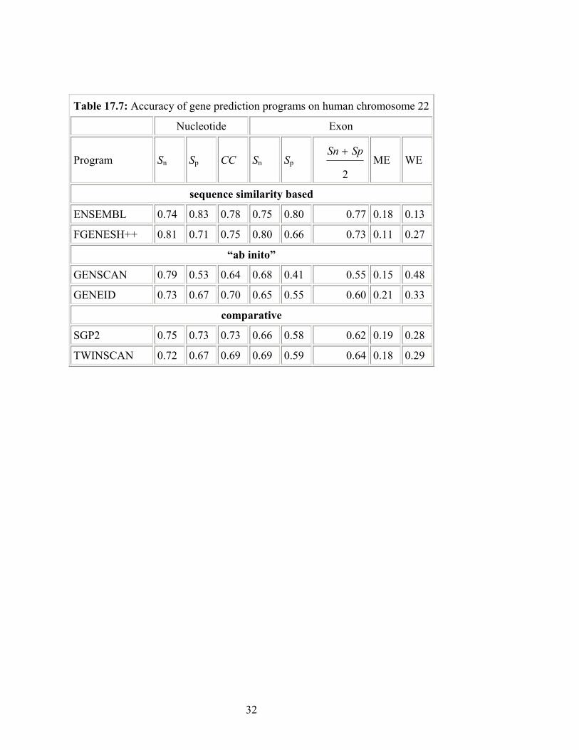
Guigó (1996) and others: gene finders were tested in controlled data sets made of short genomic sequences encoding a single gene with a simple gene structure. These data sets are not representative of the genome sequences being currently produced: large sequences of low coding density, encoding several genes and/or incomplete genes, with complex gene structure. The exhaustive scrutiniy to which the sequence of human chromosome 22 (Dunham et al., 1999) has been subjected through the Vertebrate Genome Annotation (VEGA) database project at the Sanger Center (http://vega.sanger.ac.uk/) offers in this regard, an excellent platform to obtain a more representative estimation of the accuracy of current gene finders. However, VEGA uses GENSCAN and FGENES in the annotation pipeline, and may be biased towards these programs. Table 17.7 shows the accuracy of a number of “ab initio“ and comparative gene finders in chromosome 22 when compared with the curated annotations from VEGA. Programs have been separated into categories: sequence similarity based, “ab initio“ or comparative. As can be seen, accuracy suffers substantially when moving from single gene sequences to whole chromosome sequences. For instance, GENSCAN CC drops from 0.91 in the evaluation by Rogic et al. (2001) to 0.64 for chromosome 22. But even more sophisticated gene finders, such as ENSEMBL (see section 5) or FGENESH++, which use known cDNAs and RefSeq genes, respectively, are far from producing perfect predictions, with CCs around 0.75. This numbers strongly suggest that current mammalian gene counts are still of a highly hypothetical nature. These examples demonstrate that the same program running on different datasets will often produce different results. Even running the same dataset, with the same software by different people (presumably with different way of setting the parameters for different optimization purposes or perhaps with different ways of counting positives and negatives) can result in different statistics. There can be several additional caveats when reading such accuracy estimates. Upon closer scrutiny, some false positives have turned out to be true positives after more libraries and more sensitive technologies are used . One of the fundamental reasons that no gene prediction program can give accurate total gene number is that they are all based on training statistics, hence total gene number is an intrinsically free parameter ( a normalization constant). This free parameter can be fixed (optimized) during the training process so that the total predicted gene number (or exon number) matches the total annotated (known) number in the training region. Therefore, if the training set is gene dense, the program will over predict the total for the whole genome and vice versaAnother reason has to do with the large variation of the gene sizes as has been examined more carefully by a recent study (Wang et al. 2003). It is shown that predictions of large multiple-exon genes and small single-exon genes are less reliable. The false positive is a particular serious problem for genes longer than 100kb as a long gene is more likely to be truncated into multiple shorter predicted genes (ESTs are a good way of identifying this). When the actual gene size is shorter than ~1kb, both false positive and negative predictions will rise sharply. In fact, when the predicted gene size is below 1 kb (GENSCAN), or below 10kb (FGENESH), it can be expected that most of the exons will be false positives. Since less than 4.5% genes are simple-exon genes (according to information derived from RefSeq), large multiple-exon genes are the main problem in ab initio gene predictions. Although internal exon size does not vary much, there is no typical exon number and there is no typical intron size either. It is interesting to note the mean gene size has been “evolving” from 5-10kb (before 1997), to 27kb (draft human genome in

13

2001) and to 51-59kb (finished chromosomes 14, 20 and 21 in 2003). The other three no less important reasons for not being able to obtain accurate gene numberall relate to the definition of genes. The first is the pseudo-gene (non-functional gene) and paralogous gene (duplicated gene) problems that can complicate an accurate gene count. In fact, most of the single-exon gene prediction problems are caused by the pseudo-genes, and this why unspliced ESTs are always looked upon as suspicious! The second is the overlapping, antisense or nested gene problems. The third is the alternative splicing problem. Many people define alternative transcripts as those that share exon regions, in principle this does not have to be the case. In fact some genes routinely produce transcripts containing no common exons (e.g. Titin). The bottom line is that we do not know all the rules how genes are transcribed and processed, and thus current mammalian gene catalogues are of a highly hypothetical nature. Given there is always a trade-off between false positives and false negatives, it will depend on which errors will be most detrimental, Wang et al (2003) suggest using Ensembl to control FPs (< 7%, with default parameters) and using ab initio predictions to control FNs (< 5%, with default parameters). 5. GENOME ANNOTATION SYSTEMS Currently there are three popular public human gene annotation database systems, EBI&Sanger Institute ENSEMBL (Hubbard et al. 2001, Clamp et al. 2002, http://www.ensembl.org/), UCSC Genome Browser (Kent et al. 2002, Karolchik et al. 2003, http://genome.ucsc.edu/) and NCBI LocusLink (Maglott et al 2000, Pruitt et al 2003, http://www.ncbi.nlm.nih.gov/LocusLink/). Each is associated with a native internet web browser. Fortunately, they all use the NCBI assembly of the human genome (tbuilt 33 released on April 14, 2003, Current at the time of writing).

Ensemble human genes are generated automatically by the Ensembl gene builder. For a number of chromosomes (currently chromosomes 6, 13, 14, 20 and 22), manual annotations are also available from Sanger Institute’s Vega curation system (http://vega.sanger.ac.uk/Homo_sapiens/). ENSEMBL genes are three basic types: those having full length cDNA or proteins, those having high homology to proteins in other organisms and those Genscan predicted genes matching to proteins/vertebrate mRNA and UniGene clusters. The basic gene-annotator engine (using protein homology to construct gene structure) is GENEWISE (Birney & Durbin 2000). Currently Ensembl predict 24,500 human genes (Pennisi 2003). These ‘Ensembl genes’ are regarded as being fairly conservative (with a low false positive rate), since they are all supported by experimental evidence of at least one form via sequence homology. Currently, the Ensembl project is attempting to add spliced EST information for identification of alternative transcripts and they are also incorporating comparative genomics to identify orthologs and syntenic regions.

UCSC Genome Browser provides a rapid and reliable display of any requested portion of genomes at any scale, together with dozens of aligned annotation tracks (known genes, predicted genes, ESTs, mRNAs, CpG islands, assembly gaps and coverage, chromosomal bands, mouse homologies, and more). Half of the annotation tracks are computed at UCSC from publicly available sequence data. The remaining tracks are provided by collaborators

14

worldwide. Users can also add their own custom tracks to the browser for educational or research purposes. These customizable tracks have made the Genome Browser very popular. The basic annotator engine is BLAT (Kent 2002) which allows rapid, reliable alignment of primate DNAs/RNAs or land vertebrate proteins onto the human genome, hence annotating the genome by sequence similarities. In its human gene prediction, in addition to Ensembl genes, it also displays 25,600 TWINSCAN genes, 32,400 GENEID genes, 39,800 FGENESH++ genes and 45,000 GENSCAN genes.

NCBI LocusLink has a rule-based genome annotation pipeline. Known genes are identified by aligning RefSq genes (http://www.ncbi.nlm.nih.gov/RefSeq/) and GenBank mRNAs to the genome using MegaBLAST (Zhang et al 2000). Transcript models are reconstructed by attempting to settle disagreements between individual sequence alignments without using an a priori model (such as codon usage, initiation, or polyA signals). Alternate mRNA models derived from the available mRNA and EST sequence data are grouped under the same gene when they share one or more exons on the same strand. Genes which produce non-coding transcripts are also annotated. These transcripts are annotated as "misc_RNA" features. If the defining GenBank or RefSeq sequence aligns to more than one location on the genome, the best alignment is selected and annotation made on that contig. If they are of equal quality, both are annotated. Genes (and corresponding transcript and protein features) are annotated on the contig if the defining transcript alignment is >=95% identity and the aligned region covers >=50% of the length, or at least 1000 bases. Genes predicted by GENOMESCAN are annotated only if they do not overlap any model based on a mRNA alignment. GENOMESCAN predicted 38,600 human genes from the September 2000 GoldenPath human genome sequence. In any case, the gene annotations provided by these systems are highly hypothetical, given the accuracy of currently available gene prediction programs (see Section 17.4). There is indeed a long way to go before automatic systems exist able to identify all genes in a given genomic sequence, provide the exhaustive catalogue of splice variants, and identify the sequence motifs involved in their regulation. A better understanding of what a gene is, and of the biological process involved in gene specification are certainly necessary to reach such a goal.

15

REFERENCES Abril, J.F., Guigó, R. and Wiehe, T. (2003) "gff2aplot: Plotting sequence comparisons." Bioinformatics, (in press) Altschul, S. F., Gish, W., Miller, W., Myers, E. W., and Lipman, D. (1990). Basic local alignment search tool. Journal of Molecular Biology, 215:403-410. Bafna, V. and Huson, D. H. (2000). The conserved exon method.. Proceedings of the eigth intenational conference on Intelligent Systems in Molecular Biology (ISMB, 8:3-12.) Bajic, V. (2000). Comparing the success of different prediction software in sequence analysis: A review. Briefings in Bioinformatics, 1:214-228.

Baldi, P., Brunak, S., Chauvin, Y., Andersen, C., and Nielsen, H. (2000). Assessing the accuracy of predicition algorithms for classification: an overview. Bioinformatics, 16:412-424. Batzoglou, S.,Pachter, L., Mesirov, J. P., Berger, B., and Lander, E. S. (2000). Human and mouse gene structure: Comparative analysis and application to exon prediction. Genome Research, 10(7):950-958. Bernardi G (1995) The human genome organization and evolutionary history. Annu. Rev. Genet. 29:445-476. Birney E and Durbin R (2000) Using Genewise in Drosophila annotation experiment. Genome Res. 10:547-548. Birney, E. and Durbin, R. (1997). Dynamite: a flexible code generating language for dynamic programming methods used in sequence comparison. Proceedings of the fifth intenational conference on Intelligent Systems in Molecular Biology ( ISMB, 5:56-64.) Blayo, P., Rouzé, P., and Sagot, M.-F. (2003). Orphan gene finding - an exon assembly approach. Theoretical Computer Science, 290:1407-1431 Brunak S Engelbrecht J and Knudsen S (1991) Prediction of human mRNA donor and acceptor sites from the DNA sequence. J. Mol. Biol. 220:49–65. Burge C and Karlin S (1997) Prediction of complete gene structures in human genomic DNA. J. Mol. Biol. 268:78-94. Burset M and Guigo R (1996) Evaluation of gene structure prediction programs. Genomics 34:353-367.

16

Burset M, Seledtsov IA, Solovyev VV (2000) Analysis of canonical and non-canonical splice sites in mammalian genomes. Nucleic Acids Research 28:4364-75 Castellano S., Morozova N., Morey M, Berry M.J., Serras F., Corominas M and Guigó R . (2001) in silico identification of novel selenoproteins in the Drosophila melanogaster genome. EMBO Reports 2:697-702 Castellano S, Novoselov S.V. , Kryukov GV, Lescure A , Blanco E Krol. A, Gladyshev V.N. and Guigó R. Reconsidering the evolutionary distribution of eukaryotic selenoproteins: a novel non-mammalian family with scattered phylogenetic distribution EMBO Reports, (in press) Chuang TJ, Lin WC, Lee HC, Wang CW, Hsiao KL, Wang ZH, Shieh D, Lin SC, Ch'ang LY. (2003) A complexity reduction algorithm for analysis and annotation of large genomic sequences. Genome Res. 2003 13:313-22. Clamp M et al. (2002) Ensembl 2002: accommodating comparative genomics. Nucl Acid Res. 31:38-42. Crollius, H. R., Jaillon, O., Bernot, A., Dasilva, C., Bouneau, L., Fischer, C., Fizames, C., Wincker, P., Brottier, P., Quetier, F., Saurin, W., and Weissenbach, J. (2000). Estimate of human gene number provided by genome-wide analysis using Tetraodon nigroviridis DNA sequence. Nature Genetics, 25:235-238. Dunham, I., Hunt, A. R., Collins, J. E., Bruskiewich, R., Beare, D. M., Clamp, M., Smink, L. J., Ainscough, R., Almeida, J. P., Babbage, A., et al. (1999). The DNA sequence of human chromosome 22. Nature, 402(6761):489-495. Durbin, R., Eddy, S., Crogh, A., and Mitchison, G. (1998). Biological Sequence Analysis: Probabilistic Models of Protein and Nucleic Acids. Cambridge University Press. Degroeve S, De Baets B, Van De Peer Y and Rouze P (2002) Feature subset selection for splice site prediction. Bioinformatics 18 Suppl 2:S75-S83. Dong S and Searls D (1994) Gene structure prediction by linguistic methods. Genomics 23:540-551. Fickett JW (1982) Recognition of protein coding regions in DNA sequences. Nucl. Aid. Res. 10:5303-5318. Fickett JW and Tung CS (1992) Assessment of protein coding measures. Nucl Acid Res. 20:6441-6450. Florea, L., Hartzell, G., Zhang, Z., Rubin, G. M., and Miller, W. (1998). A computer program for aligning a cDNA sequence with a genomic DNA sequence. Genome Research, 8(9):967-974.

17

Gelfand M and Roytberg M (1993) Prediction of exon-intron structure by a dynamic programming approach. BioSystems 30:173-182. Gelfand, M. S., Mironov, A. A., and Pevzner, P. A. (1996). Gene recognition via spliced alignment. Proceedings National Academy Sciences USA, 93:9061-9066. Gish, W. and States, D. (1993). Identification of protein coding regions by database similarity search. Nature Genetics, 3:266-272. Guigo R, Knudsen S, Drake N and Smith T (1992) Prediction of gene structure. J. Mol. Biol. 266:141-157. Guigó, R. (1998). Assembling genes from predicted exons in linear time with dynamic programming. Journal of Computational Biology, 5:681-702.

Guigó, R (1999) "DNA composition, codon usage and exon prediction." In M. Bishop, editor: Genetic Databases. Pp:53-80. Academic Press.

Guigó, R. and Wiehe, T. (2003). Gene prediction accuracy in large DNA sequences. In Galperin, M. Y. and Koonin, E. V., editors, Frontiers in Computational Genomic. Caister Academic Press. Guigó R, Dermitzakis E.T, Agarwal P, Ponting C.P, Parra G., Reymond A, Abril J.F, Keibler E, Lyle R, Ucla C., Antonarakis SE and Brent MR (2003) Comparison of mouse and human genomes followed by experimental verification yields an estimated 1,019 additional genes. Proc. Nat. Acad. Sci. 100:1140-1145 Henderson J, Salzberg S and Fasman KH (1997) Finding genes in DNA with a Hidden Markov Model. J Comput Biol. 4:127-141. Hubbard D et al. (2001) The Ensembl genome database project. Nucl Acid Res. 30:38-41. Hutchinson GB and Hayden MR (1992) The prediction of exons through an analysis of splicible open reading frames. Nucl Acid Res. 20:3452-3462. Karolchik D, Baertsch R, Diekhans M, Furey TS, Hinrichs A, Lu YT, Roskin KM, Schwartz M, Sugnet CW, Thomas DJ, Webwe RJ, Haussler D, Kent WJ (2003) The UCSC Genome Browser Databse. Nucl Acid Res. 31:51-54. Kent WJ (2002) BLAT – The Blast-like alignment tool. Genome Res. 12:4656-4664. Kent WJ, Sugnet CW, Furey TS, Roskin KM, Pringle TH, Zahler AM and Haussler D (2002) The human genome browser at UCSC. Genome Res. 12:996-1006.

18

Korf I, Flicek P, Duan D and Brent MR. (2001) Integrating genomic homology into gene structure prediction. Bioinformatics 17 Suppl 1, S140-148. Kozak M (1987) An analysis of 5’-noncoding sequences from 699 vertebrate messenger RNAs. Nucl. Acid. Res. 15:8125-8132. Kryukov GV, Castellano S., Novoselov SV, Lobanov AV, Zehtab O, Guigó R and Gladyshev VN (2003) "Characterization of mammalian selenoproteomes." Science 300:1439-1443 Krogh A (1997) Two methods for improving performance of an HMM and their application for gene finding. Proc Int Conf Intell Syst Mol Biol. 5:179-186. Krogh A, Mian IS and Haussler D (1994) A hidden Markov model that finds genes in E. coli DNA. Nucl Acid Res. 22:4768-4778. Kulp D, Haussler D, Reese MG and Eeckman F (1996) A generalized hidden Markov model for the recognition of human genes in DNA. Proc Int Conf Intell Syst Mol Biol. 4:134-142. Lapedes A, Barnes C, Burks C, Farber R and Sirotkin K (1990) Application of neural networks and other machine learning algorithms to DNA sequence analysis. In Computers and DNA, Bell GI and Marr TG eds, pp157-182. Addison-Wesley, New York. Lim LP and Burge CB (2001) A computational analysis of sequence features involved in recognition of short introns. Proc Natl Acad Sci USA, 98:11193-11198. Mache,N. and Levi,P. (1998) GENIO—A Non-Redundant Eukaryotic Gene Database of Annotated Sites and sequences. RECOMB-98 Poster, New York. Maglott DR, Katz KS, Sicotte H and Pruitt KD (2000) NCBI’s LocusLink and RefSeq. Nucl Acid Res. 28:126-128. Meyer, I.M. and Durbin, R. (2002). Comparative ab initio prediction of gene structures using pair HMMs. Bioinformatics, 18(10):1309-1318. Miller, W. (2001). Comparison of genomic DNA sequences: solved and unsolved problems. Bioinformatics, 17:391-397. Mount SM (1982) A catalogue of splice junction sequences. Nucl. Acid. Res. 10:459-472. Mott, R. (1997). EST_GENOME: a program to align spliced DNA sequences to unspliced genomic DNA. Computer Applications in the Biosciences, 13:477-478.

19

Pachter, L., Alexandersson, M., and Cawley, S. (2002). Applications of Generalized Pair Hidden Markov Models to Alignment and Gene Finding Problems. Journal of Computational Biology, 9(2):389-400. Parra G, Blanco E, and Guigó R. (2000) "Geneid in Drosophila." Genome Research 10:511-515 Parra G, Agarwal P, Abril JF, Wiehe T, Fickett JW and Guigó R (2003) Comparative gene prediction in human and mouse. Genome Research 13:108-117 Patterson DJ, Yasuhara K and Ruzzo WL (2002) Pre-mRNA secondary structure prediction aids splice site prediction. Pac. Symp. Biocomput. 2002:223-234. Pearson, W. R. (1999). Flexible similarity searching with the Fasta3 program package. In Misener, S. and Krawetz, S. A., editors, Bioinformatics Methods and Protocols, pages 185-219, Totowa, New Jersey. Humana Press. Pedersen, C. and Scharl, T. (2002). Comparative methods for gene structure prediction in homologous sequences. In Guigó, R. and Gusfield, D., editors, Algorithms in ioinformatics. Pennisi E (2003) Gene counters struggle to get the right answer. Science 301:1040-1041. Pertea M, Lin X and Salzberg SL (2001) GeneSplicer: a new computational method for splice site prediction. Nucl. Acid.Res. 29:1185-1190. Pruitt KD, Tatusov T and Maglott DR (2003) RefSeq and LocusLink: NCBI gene-centered resources. Nucl Acid Res. 31:34-37. Rabiner LR (1989) A tutorial on hidden Markov models and selected applications in speech recognition. Proc. IEEE 77:257-286. Reese MG, Eeckman FH, Kulp D and Haussler D (1997) Improved splice site detection in Genie. J. Comput. Biol. 4:311–323. Robbertson BL, Cote GJ and Berget SM (1990) Exon definition may facilitate splice site selection in RNAs with multiple exons. Mol Cell Biol. 10:84-94. Rogic S, Mackworth AK and Ouellette FB (2001) Evaluation of gene-finding programs on mammalian sequences. Genome Res.11:817-832. Rogozin IB and Milanesi L (1997) Analysis of donor splice signals in different organisms. J. Mol. Evol., 45:50–59. Samalov AA and Solovyev VV (2000) Ab initio gene finding in Drosophila genomic DNA. Genome Res. 10:516-522.

20

Salsberg S, Delcher A, Fasman K and Henderson J (1998) A decision tree system for finding genes in DNA. J. Comp. Biol. 5:667-680. Senapathy P, Shapiro MB and Harris NL (1990) Splice junctions, branch point sites, and exons: sequence statistics, identification and genome project. Met. Enz. 183:252-278. Snyder EE and Stormo GD (1993) Identification of coding regions in genomic DNA sequences: an application of dynamic programming and neural networks. Nucl Acid Res. 21:607-613. Snyder EE and Stormo GD (1995) Identification of protein coding regions in genomic DNA. J Mol Biol. 248:1-18 Solovyev VV, Salamov AA and Lawrence CB (1994) Predicting internal exons by oligonucleotide composition and discriminant analysis of spliceable open reading frames. Nucleic Acids Res. 22:5156-5163. Solovyev VV, Salamov AA and Lawrence CB (1995) Prediction of human gene structure using linear discriminant functions and dynamic programming. In Proc. of the Third International Conference on Intelligent Systems for Molecular Biology, Rawling C et al. eds. Cambridge, Eng.: AAAI Press, pp367-375. Solovyev VV, Salamov AA and Lawrence CB (1995) The gene-finding computer tools for analysis of human and model organisms genome sequences. In Proc. of the 5th International Conference on Intelligent Systems for Molecular Biology, Rawling C et al. eds. Cambridge, Eng.: AAAI Press, pp294-302 Solovyev VV (2002) Finding genes by computer. In Current Topics in Computational Molecular Biology. Jing T, Xu Y and Zhang MQ eds., pp201-248. The MIT Press. Cambridge, MA. Staden R (1984) Computer methods to locate signals in nucleic acid sequences. Nucl. Acid. Res. 12:505-519. Staden R and McLachlan AD (1982) Codon preference and its use in identifying protein coding regions in long DNA sequences. Nucl. Acid. Res. 10:141-156. Thanaraj TA and Robinson AJ (2000) Prediction of exact boundaries of exons. Nucl. Acid. Res. 1:343-56 Thomas A and Skolnick M (1994) A probabilistic model for detecting coding regions in DNA sequences. IMAJ. Math Appl Med Biol. 11:149-160. Usuka, J. and Brendel, V. (2000). Gene structure prediction by spliced alignment of genomic DNA with protein sequences: increased accuracy by differential splice site scoring. Journal of Molecular Biology, 297:1075-1085.

21

Wang J, Li ST, Zhang Y, Zheng HK, Xu Z, Ye J, Yu J and Wong GK (2003) Opinion: Vertebrate gene predictions and the problem of large genes. Nat Rev Genet. 4:741-749. Wiehe, T., Gebauer-Jung, S., Mitchell-Olds, T., and Guigó, R. (2001). SGP-1: Prediction and validation of homologous genes based on sequence alignments. Genome Research, 11:1574-1583. Xu Y, Einstein JR, Mural RJ, Shah M and Uberbacher EC (1994) An improved system for exon recognition and gene modeling in human DNA sequences. In Proc. of the 2nd Intl Conf. Intel. Sys for Mol Biol, Altman et al eds., Cambridge, UK: AAAI Press, 376-383. Yada T, Takagi T, Totoki Y, Sakaki Y and Takaeda Y (2003) DIGIT: a novel gene finding program by combining gene-finders. Pac Symp Biocomput. 2003:375-387. Yeh RF, Lim LP and Burge CB (2001) Computational inference of homologous gene structures in the human genome. Genome Res.11:803-816. Zhang MQ (1993) A weight array method for splicing signal analysis. CABIOS 9:499-509. Zhang MQ (1997) Identification of protein coding regions in the human genome based on quadratic discriminant analysis. Proc. Natl Acad Sci USA 94:565-568. Zhang MQ (1998) Statistical Features of Human Exons and Their Flanking Regions. Hum. Mol. Genet., 7:919-932. Zhang MQ (2000) Discriminant analysis and its application in DNA sequence motif recognition. in Briefings in Bioinformatics 1(4):331-342. Zhang MQ (2002) Computational prediction of eukaryotic protein-coding genes. Nat. Rev. Genet. 3:698-709. Zhang Z, Schwartz S, Wagner L and Miller W (2000) A greedy algorithm for aligning DNA sequences. J Comput Biol 7:203-214.

22

FIGURES and TABLES

Figure 17.1 A gene organization that has 6 exons

Promoter

transcriptionalinitiation site

translationalstart site

translationalstop site

poly(A)site

transcriptionaltermination site

5’ 3’

Gene

5’UTR 3’UTRCDS

mRNA transcript

Cap AAA...AA tail

23

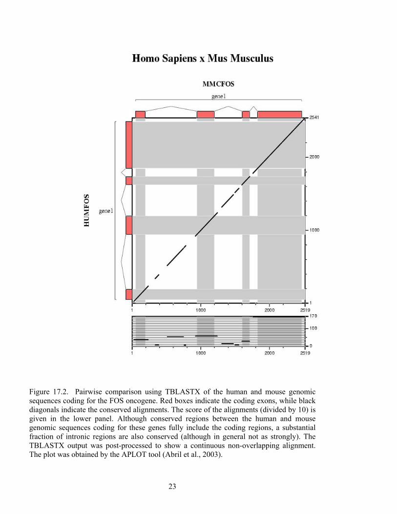
Figure 17.2. Pairwise comparison using TBLASTX of the human and mouse genomic sequences coding for the FOS oncogene. Red boxes indicate the coding exons, while black diagonals indicate the conserved alignments. The score of the alignments (divided by 10) is given in the lower panel. Although conserved regions between the human and mouse genomic sequences coding for these genes fully include the coding regions, a substantial fraction of intronic regions are also conserved (although in general not as strongly). The TBLASTX output was post-processed to show a continuous non-overlapping alignment. The plot was obtained by the APLOT tool (Abril et al., 2003).

24

Figure 17.3. Multiple sequence alignment of different members of SelU, a novel selenoprotein family predicted after computational analysis that involved genome sequence comparisons between human and fugu. SelU is a selenoprotein in Fugu (the sequences of two members of the family, SelUa and SelUb are included in the alignment) but not in human, where the members of this family use Cysteine instead of Selenocysteine (denoted by the letter U in the amino acid one letter code). After the prediction of SelU as a potential selenoprotein, exhaustive sequence similarity searches were performed against transcript sequences, and found members of this family across the whole eukaryotic spectrum; as the intial analysis suggested, SelU is a selenoprotein in some eukaryotic species, and it is not in others. Strong sequence conservation across the U residue (encoded by TGA, otherwise a stop codon) strongly suggest this to be a "bona fide" selenoprotein, instead of a false positive. This selenoprotein was later verified by radioactive labelling of Selenium. The pattern Sec-X-X-Cys is not uncommon in selenoproteins. (Adapted from Castellano et al., in press).

25

Table 17.1. Donor (from human), Acceptor (from human) and Branch Point (from human, rat, chicken, plant and drosophila) frequency matrices (Senapathy et al, 1990).

Donor frequency matrix position -3 –2 –1 | +1 +2 +3 +4 +5 +6A 28 59 8 | 0 0 54 74 5 16C 40 14 5 | 0 0 2 8 6 18G 17 13 81 | 100 0 42 11 85 21T 14 14 6 | 0 100 2 8 4 45

Acceptor frequency matrix position -14 –13 –12 –11 –10 -9 -8 -7 -6 -5 -4 -3 -2 -1 | +1 A 10 8 6 6 9 9 8 9 6 6 23 2 100 0 | 28 C 31 36 34 34 37 38 44 41 44 40 28 79 0 0 | 14 G 14 14 12 8 9 10 9 8 6 6 26 1 0 100 | 47 T 44 43 48 52 45 44 40 41 45 48 23 18 0 0 | 11

Branch frequency matrix position -3 –2 –1 0 +1 A 1 0 39 99 11 C 76 8 15 1 45 G 2 0 42 0 6 T 21 91 4 0 38

26

Table 17.2. GC-specific (low/high) Donor, Acceptor and Branch Point (all from human) frequency matrices (Zhang, 1998). Donor:

Acceptor: -15 -14 -13 -12 -11 -10 -9 -8 A 15/10 14/8 13/7 11/8 10/6 10/6 11/4 12/8 C 24/41 21/42 20/41 22/40 21/38 22/43 25/42 28/46 G 10/15 12/14 10/14 9/13 10/13 9/12 10/13 10/14 T 51/34 53/36 57/38 58/30 59/43 59/39 54/41 50/32 -7 -6 -5 -4 -3 -2 -1 +1 +2 13/8 11/7 10/6 26/19 7/2 100 0 26/21 24/19 28/49 25/54 22/45 25/38 55/82 0 0 11/13 15/21 8/10 5/8 5/8 15/26 1/0 0 100 50/58 20/29 51/33 59/31 63/41 33/17 37/16 0 0 13/8 41/31 Branch site -5 -4 -3 -2 -1 0 +1 A 25/15 25/15 0 0 39/16 100 18/7 C 19/36 22/38 66/88 2/5 24/31 0 33/56 G 15/24 17/22 0 0 32/51 0 3/12 T 41/25 36/25 40/12 98/95 5/2 0 46/25

-3 -2 -1 +1 +2 +3 +4 +5 +6 A 38/32 62/55 12/8 0 0 71/38 73/70 11/5 21/13 C 31/38 10/15 4/4 0 0 2/4 6/9 6/5 10/21 G 18/19 12/15 77/80 100 0 24/56 8/14 75/86 14/25 T 13/11 16/14 7/8 0 100 3/2 13/7 8/4 55/41

27

Table 17.3: Accuracy of exon prediction methods

Nucleotide Exon

Program Sn Sp CC Sn Sp 2

SpSn +

GRAIL2 0.79 0.92 0.83 0.53 0.60 0.57

FGENEH 0.83 0.93 0.85 0.73 0.78 0.76

MZEF 0.87 0.95 0.89 0.78 0.86 0.82

28

Table 17.4.

Table 4. Useful internet gene prediction resources Weintian Li’s Bibliography on Computational Gene Recognition

http://www.nslij-genetics.org/gene/

BCM Search Launcher: many gene finding programs

http://dot.imgen.bcm.tmc.edu:9331/seq-search/gene-search.html

PROMOTER RECOGNITION NNPP: ANN promoter prediction http://www.fruitfly.org/seq_tools/promoter.html PromoterInspector; MatInspector; FastM; SMARTest

http://genomatix.gsf.de/software_services/free_access/free_accounts.html

Signal Scan: TFD or TRANSFAC http://bimas.dcrt.nih.gov/molbio/signal/ TESS: Transcription Factor site search http://www.cbil.upenn.edu/tess/ TFBIND: Trasncription Factor site search http://tfbind.ims.u-tokyo.ac.jp/ Core-Promoter: Transcription Start Site prediction http://argon.cshl.org/genefinder/CPROMOTER/ Dragon Promoter Finder http://sdmc.lit.org.sg/promoter/promoter1_3/DPFV13.htm Promoter: Transcription Start Site prediction http://www.cbs.dtu.dk/services/Promoter/

SPLICE SITE PREDICTION NetGene2: Splice sites in human, C. elegans and Arabidopsis

http://www.cbs.dtu.dk/services/NetGene2/

NNSplice: ANN, splice site prediction http://www.fruitfly.org/seq_tools/splice.html SplicePredictor http://bioinformatics.iastate.edu/cgi-bin/sp.cgi GeneSplicer http://www.tigr.org/tdb/GeneSplicer/gene_spl.html SpliceView http://l25.itba.mi.cnr.it/~webgene/wwwspliceview_help.html RNASPL http://www.dl.ac.uk/CCP/CCP11/DISguISE/nucleotide_analysis/rnasplwww.html

GENE PREDICTION AAT: MZEF+homology http://genome.cs.mtu.edu/aat.html CDS: search coding region http://bioweb.pasteur.fr/seqanal/interfaces/cds-simple.html CRASA: EST based gene finder http://crasa.sinica.edu.tw/bioinformatics/introduce.html DioGenes: finding orfs in short genomic sequences http://www.cbc.umn.edu/diogenes/index.html Fgenesh: HMM (human, Drosophila, dicots, monocots, C. elegans, S.pombe); Fgenes; Hexon; TSSW; TSSG; SPL; Polyah

http://genomic.sanger.ac.uk/gf/gf.shtml http://searchlauncher.bcm.tmc.edu:9331/seq-search/gene-search.html http://www.softberry.com/nucleo.html

FirstEF; Core_Promoter; CpG_Promoter; Polyadq; JTEF;

http://www.cshl.edu/mzhanglab/

GeneID: Hierarchical rules (human, Drosophila) http://www1.imim.es/software/geneid/geneid.html#top GeneMachine: integrated gene finder http://genome.nhgri.nih.gov/genemachine/ GeneMark: include HMM (many species) http://dot.imgen.bcm.tmc.edu:9331/seq-search/gene-search.html GeneParser: Dynamic Programming (DP)-ANN http://beagle.colorado.edu/~eesnyder/GeneParser.html GeneSeqer: EST-based gene prediction http://bioinformatics.iastate.edu/cgi-bin/gs.cgi GeneWise2: DNA protein alignment http://www.cbil.upenn.edu/tess/ Genie: HMM (human, Drosophila) http://www.fruitfly.org/seq_tools/genie.html GenLang: Linguistic grammer http://www.cbil.upenn.edu/genlang/genlang_home.html Genomescan: HMM+protein similarity (human, Arabidopsis, maize)

http://genes.mit.edu/genomescan/

Genscan: HMM (human, Arabidopsis, maize) http://genes.mit.edu/GENSCAN.html GRAIL: ANN (human, mouse, Drosophila, Arabidopsis)

http://compbio.ornl.gov/tools/index.shtml

HMM-gene: HMM (human, C. elegans) http://www.cbs.dtu.dk/services/HMMgene MORGAN: tree; VEIL: HMM; GLIMMER: IMM (micro.)

http://www.tigr.org/~salzberg/

MZEF SPC: MZEF+SpliceProximalCheck http://industry.ebi.ac.uk/~thanaraj/MZEF-SPC.html MZEF: QDA (human, mouse, Arabidopsis); POMBE: LDA

http://www.cshl.edu/mzhanglab/

OrfFinder http://www.ncbi.nlm.nih.gov/gorf/gorf.html PredictGenes http://cbrg.inf.ethz.ch/subsection3_1_8.html Procrustes: splice alignment http://www-hto.usc.edu/software/procrustes/index.html SLAM: Dual HMM (human-mouse syntenic regions)

http://bio.math.berkeley.edu/slam/

Twinscan: Genscan+conservation sequence http://genes.cs.wustl.edu/ WebGene: DP (human, mouse, Fugu, Drosophila, C. elegans, Arabidopsis, Aspergillus)

http://www.itba.mi.cnr.it/webgene/

29

Xpound ftp://igs-server.cnrs-mrs.fr/pub/Banbury/xpound/ YeastGene http://tubic.tju.edu.cn/cgi-bin/Yeastgene.cgi VEIL HMM http://www.tigr.org/~salzberg/veil.html EST_Genome: aligns cDNA to DNA http://www.well.ox.ac.uk/~rmott/est_genome.shtml TAP: EST-based gene prediction http://sapiens.wustl.edu/~zkan/TAP/ EbEST: EST-based gene prediction http://rgd.mcw.edu/EBEST/ SGP1: comparative gene prediction http://195.37.47.237/sgp-1/ SGP2: comparative gene prediction http://genome.imim.es/software/sgp2/

30

Table 17.5: Accuracy of gene predictions programs on single gene vertebrate sequences. Adapted from Burset and Guigó (1996)

Nucleotide Exon

Program Dataset Sn Sp CC Sn Sp 2

SpSn + ME WE

FGENEH ALLSEQ 0.77 0.88 0.80 0.61 0.64 0.64 0.15 0.12

NEWSEQ 0.70 0.83 0.73 0.51 0.54 0.54 0.22 0.18

GENEID ALLSEQ 0.63 0.81 0.65 0.44 0.46 0.45 0.28 0.24

NEWSEQ 0.58 0.78 0.60 0.41 0.43 0.42 0.34 0.27

GENEPARSER2 ALLSEQ 0.66 0.79 0.65 0.35 0.40 0.37 0.29 0.17

NEWSEQ 0.63 0.76 0.62 0.33 0.39 0.36 0.32 0.20

GENLANG ALLSEQ 0.72 0.79 0.71 0.51 0.52 0.52 0.21 0.22

NEWSEQ 0.63 0.73 0.63 0.39 0.44 0.43 0.29 0.25

GRAIL 2 ALLSEQ 0.72 0.87 0.76 0.36 0.43 0.40 0.25 0.11

NEWSEQ 0.69 0.85 0.72 0.34 0.41 0.38 0.30 0.13

SORFIND ALLSEQ 0.71 0.85 0.72 0.42 0.47 0.45 0.24 0.14

NEWSEQ 0.65 0.79 0.65 0.36 0.39 0.38 0.29 0.19

XPOUND ALLSEQ 0.61 0.87 0.69 0.15 0.18 0.17 0.33 0.13

NEWSEQ 0.58 0.83 0.64 0.12 0.15 0.14 0.36 0.16

GENEID+ ALLSEQ 0.91 0.91 0.88 0.73 0.70 0.71 0.07 0.13

NEWSEQ 0.88 0.87 0.84 0.68 0.64 0.66 0.10 0.15

GENEPARSER3 ALLSEQ 0.86 0.91 0.85 0.56 0.58 0.57 0.14 0.09

NEWSEQ 0.83 0.89 0.82 0.50 0.53 0.51 0.17 0.09

31

Table 17.6: Accuracy of gene prediction programs on single gene mammalian sequences. Adapted from Rogic et al. (2001)

Nucleotide Exon

Program Sn Sp CC Sn Sp 2

SpSn +ME WE

FGENES 0.86 0.88 0.83 0.67 0.67 0.67 0.12 0.09

GENEMARK.hmm 0.87 0.89 0.83 0.53 0.54 0.54 0.13 0.11

GENIE 0.91 0.90 0.88 0.71 0.70 0.71 0.19 0.11

GENSCAN 0.95 0.90 0.91 0.70 0.70 0.70 0.08 0.09

HMMGENE 0.93 0.93 0.91 0.76 0.77 0.76 0.12 0.07

MORGAN 0.75 0.74 0.69 0.46 0.41 0.43 0.20 0.28

MZEF 0.70 0.73 0.66 0.58 0.59 0.59 0.32 0.23

32

Table 17.7: Accuracy of gene prediction programs on human chromosome 22

Nucleotide Exon

Program Sn Sp CC Sn Sp 2

SpSn +ME WE

sequence similarity based

ENSEMBL 0.74 0.83 0.78 0.75 0.80 0.77 0.18 0.13

FGENESH++ 0.81 0.71 0.75 0.80 0.66 0.73 0.11 0.27

“ab inito”

GENSCAN 0.79 0.53 0.64 0.68 0.41 0.55 0.15 0.48

GENEID 0.73 0.67 0.70 0.65 0.55 0.60 0.21 0.33

comparative

SGP2 0.75 0.73 0.73 0.66 0.58 0.62 0.19 0.28

TWINSCAN 0.72 0.67 0.69 0.69 0.59 0.64 0.18 0.29