chapter 17: exploratory factor analysis - sage publicationschapter 17: exploratory factor analysis...
TRANSCRIPT

DISCOVERING STATISTICS USING SPSS
PROFESSOR ANDY P FIELD 1
Chapter 17: Exploratory factor analysis
Smart Alex’s Solutions
Task 1
Rerun the analysis in this chapter using principal component analysis and compare the results to those in the chapter. (Set the iterations to convergence to 30.)
Running the analysis
Access the main dialog box (Figure 1) by selecting . Simply select the variables you want to include in the analysis (remember to exclude any variables that were identified as problematic during the data screening) and transfer them to the box labelled Variables by clicking on .
Figure 1: Main dialog box for factor analysis
There are several options available, the first of which can be accessed by clicking on to access the dialog box in Figure 2. The Univariate descriptives option provides
means and standard deviations for each variable. Most of the other options relate to the correlation matrix of variables (the R-‐matrix). The Coefficients option produces the R-‐matrix, and selecting the Significance levels option will include the significance value of each correlation in the R-‐matrix. You can also ask for the Determinant of this matrix, and this option is useful for testing for multicollinearity or singularity.
KMO and Bartlett’s test of sphericity produces the Kaiser–Meyer–Olkin measure of sampling adequacy and Bartlett’s test. We have already stumbled across KMO and Bartlett’s test and have seen the various criteria for adequacy, but with a sample of 2571 we shouldn’t have cause to worry.

DISCOVERING STATISTICS USING SPSS
PROFESSOR ANDY P FIELD 2
The Reproduced option produces a correlation matrix based on the model (rather than the real data). Differences between the matrix based on the model and the matrix based on the observed data indicate the residuals of the model. SPSS produces these residuals in the lower table of the reproduced matrix, and we want relatively few of these values to be greater than .05. Luckily, to save us scanning this matrix, SPSS produces a summary of how many residuals lie above .05. The Reproduced option should be selected to obtain this summary. The Anti-‐image option produces an anti-‐image matrix of covariances and correlations. These matrices contain measures of sampling adequacy for each variable along the diagonal and the negatives of the partial correlation/covariances on the off-‐diagonals. The diagonal elements, like the KMO measure, should all be greater than 0.5 at a bare minimum if the sample is adequate for a given pair of variables. If any pair of variables has a value less than this, consider dropping one of them from the analysis. The off-‐diagonal elements should all be very small (close to zero) in a good model. When you have finished with this dialog box click on to return to the main dialog box.
Figure 2: Descriptives in factor analysis
To access the extraction dialog box (Figure 3), click on in the main dialog box. There are several ways of conducting a factor analysis, and when and where you use the various methods will depend on numerous things. For our purposes we will use principal component analysis ( ) which, strictly speaking, isn’t factor analysis; however, the two procedures may often yield similar results.
In the Analyze box there are two options: to analyse the Correlation matrix or to analyse the Covariance matrix. The Display box has two options within it: to display the Unrotated factor solution and a Scree plot. The scree plot is a useful way of establishing how many factors should be retained in an analysis. The unrotated factor solution is useful in assessing the improvement of interpretation due to rotation. If the rotated solution is little better than the unrotated solution then it is possible that an inappropriate (or less optimal) rotation method has been used.
DISCOVERING STATISTICS USING SPSS
PROFESSOR ANDY P FIELD 3
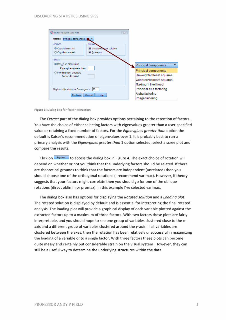
Figure 3: Dialog box for factor extraction
The Extract part of the dialog box provides options pertaining to the retention of factors. You have the choice of either selecting factors with eigenvalues greater than a user-‐specified value or retaining a fixed number of factors. For the Eigenvalues greater than option the default is Kaiser’s recommendation of eigenvalues over 1. It is probably best to run a primary analysis with the Eigenvalues greater than 1 option selected, select a scree plot and compare the results.
Click on to access the dialog box in Figure 4. The exact choice of rotation will depend on whether or not you think that the underlying factors should be related. If there are theoretical grounds to think that the factors are independent (unrelated) then you should choose one of the orthogonal rotations (I recommend varimax). However, if theory suggests that your factors might correlate then you should go for one of the oblique rotations (direct oblimin or promax). In this example I’ve selected varimax.
The dialog box also has options for displaying the Rotated solution and a Loading plot. The rotated solution is displayed by default and is essential for interpreting the final rotated analysis. The loading plot will provide a graphical display of each variable plotted against the extracted factors up to a maximum of three factors. With two factors these plots are fairly interpretable, and you should hope to see one group of variables clustered close to the x-‐axis and a different group of variables clustered around the y-‐axis. If all variables are clustered between the axes, then the rotation has been relatively unsuccessful in maximizing the loading of a variable onto a single factor. With three factors these plots can become quite messy and certainly put considerable strain on the visual system! However, they can still be a useful way to determine the underlying structures within the data.
DISCOVERING STATISTICS USING SPSS
PROFESSOR ANDY P FIELD 4
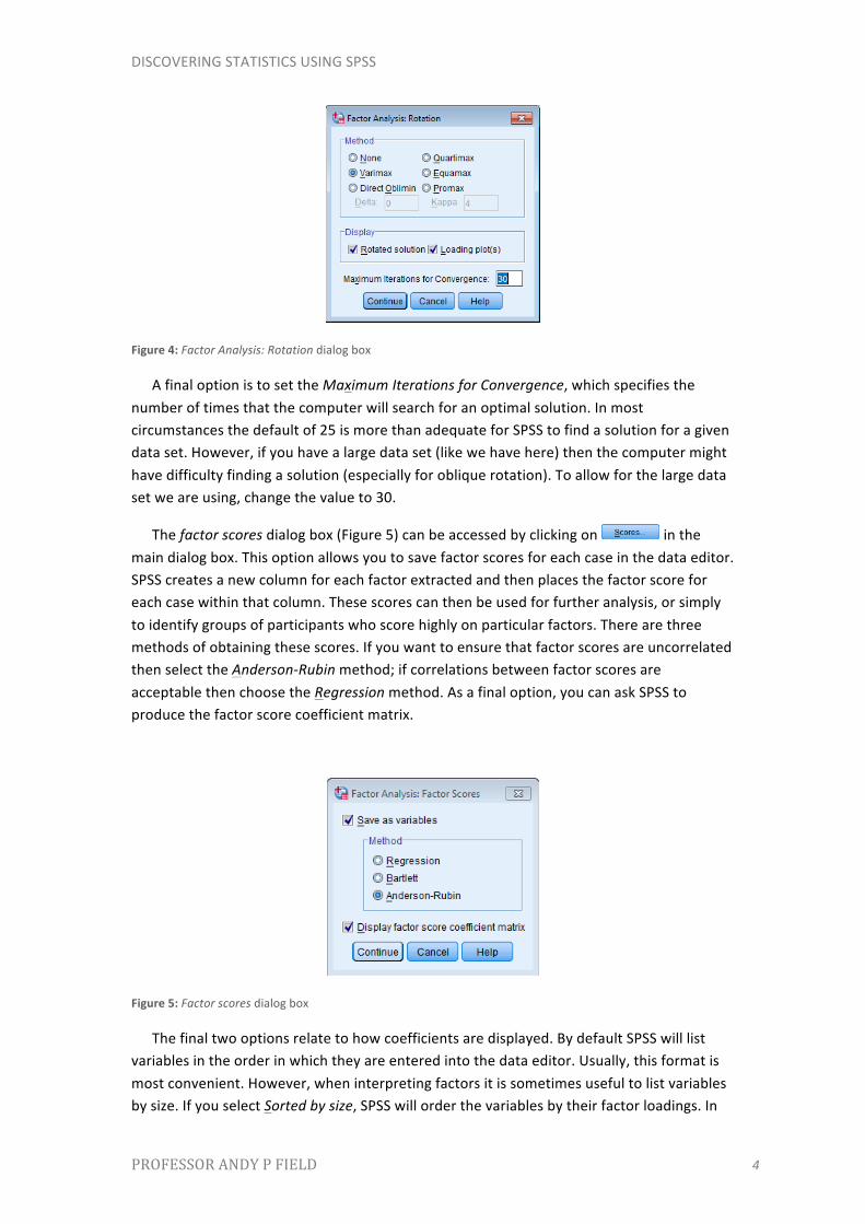
Figure 4: Factor Analysis: Rotation dialog box
A final option is to set the Maximum Iterations for Convergence, which specifies the number of times that the computer will search for an optimal solution. In most circumstances the default of 25 is more than adequate for SPSS to find a solution for a given data set. However, if you have a large data set (like we have here) then the computer might have difficulty finding a solution (especially for oblique rotation). To allow for the large data set we are using, change the value to 30.
The factor scores dialog box (Figure 5) can be accessed by clicking on in the main dialog box. This option allows you to save factor scores for each case in the data editor. SPSS creates a new column for each factor extracted and then places the factor score for each case within that column. These scores can then be used for further analysis, or simply to identify groups of participants who score highly on particular factors. There are three methods of obtaining these scores. If you want to ensure that factor scores are uncorrelated then select the Anderson-‐Rubin method; if correlations between factor scores are acceptable then choose the Regression method. As a final option, you can ask SPSS to produce the factor score coefficient matrix.
Figure 5: Factor scores dialog box
The final two options relate to how coefficients are displayed. By default SPSS will list variables in the order in which they are entered into the data editor. Usually, this format is most convenient. However, when interpreting factors it is sometimes useful to list variables by size. If you select Sorted by size, SPSS will order the variables by their factor loadings. In

DISCOVERING STATISTICS USING SPSS
PROFESSOR ANDY P FIELD 5
fact, it does this sorting fairly intelligently so that all of the variables that load highly onto the same factor are displayed together. The second option is to Suppress small coefficients: Absolute value below a specified value (by default .1). This option ensures that factor loadings within ± .1 are not displayed in the output. Again, this option is useful for assisting in interpretation. The default value is probably sensible, but on your first analysis I recommend changing it either to .4 (for interpretation purposes) or to a value reflecting the expected value of a significant factor loading given the sample size. This will make interpretation simpler. You can, if you like, rerun the analysis and set this value lower just to check you haven’t missed anything (like a loading of .39). For this example set the value at .4.
Figure 6: Factor analysis options dialog box
Interpreting output from SPSS
Select the same options as I have in the screenshots and run a PCA with orthogonal rotation. Repeat, but using direct oblimin rotation. For the purposes of saving space in this section I set the default SPSS options such that each variable is referred to only by its label on the data editor (e.g., Q12). On the output you obtain, you should find that the SPSS uses the value label (the question itself) in all of the output. When using the output in this chapter just remember that Q1 represents question 1, Q2 represents question 2 and Q17 represents question 17.
The first body of output concerns data screening, assumption testing and sampling adequacy. You’ll find several large tables (or matrices) that tell us interesting things about our data. If you selected the Univariate descriptives option in Figure 2 then the first table will contain descriptive statistics for each variable (the mean, standard deviation and number of cases). This table is not included here, but you should have enough experience to be able to interpret it. The table also includes the number of missing cases; this summary is a useful way to determine the extent of missing data.
The top half of the R-‐matrix (or correlation matrix) shows the Pearson correlation coefficient between all pairs of questions, whereas the bottom half contains the one-‐tailed

DISCOVERING STATISTICS USING SPSS
PROFESSOR ANDY P FIELD 6
significance of these coefficients (Output 1). We can use this correlation matrix to check the pattern of relationships. First, scan the matrix for correlations greater than .3, then look for variables that only have a small number of correlations greater than this value. Then scan the correlation coefficients themselves and look for any greater than .9. If any are found then you should be aware that a problem could arise because of multicollinearity in the data.
In summary, all questions in the SAQ correlate reasonably well with all others and none of the correlation coefficients are excessively large; therefore, we won’t eliminate any questions at this stage.
Output 1
Output shows the inverse of the correlation matrix (R−1), which is used in various calculations (including factor scores). This matrix is produced using the Inverse option in Figure 2 but in all honesty is useful only if you want some insight into the calculations that go on in a factor analysis. Most of us have more interesting things to do than gain insight into the workings of factor analysis and the practical use of this matrix is minimal—so ignore it!
Output shows several very important parts of the output: the KMO measure of sampling adequacy, Bartlett’s test of sphericity and the anti-‐image correlation and covariance matrices (note that these matrices have been edited down to contain only the first and last
Correlation Matrixa
1.000-.099-.337.436.402-.189.214.329-.104-.004-.0991.000.318-.112-.119.203-.202-.205.231.100-.337.3181.000-.380-.310.342-.325-.417.204.150.436-.112-.3801.000.401-.186.243.410-.098-.034.402-.119-.310.4011.000-.165.200.335-.133-.042.217-.074-.227.278.257-.167.101.272-.165-.069.305-.159-.382.409.339-.269.221.483-.168-.070.331-.050-.259.349.269-.159.175.296-.079-.050
-.092.315.300-.125-.096.249-.159-.136.257.171.214-.084-.193.216.258-.127.084.193-.131-.062.357-.144-.351.369.298-.200.255.346-.162-.086.345-.195-.410.442.347-.267.298.441-.167-.046.355-.143-.318.344.302-.227.204.374-.195-.053.338-.165-.371.351.315-.254.226.399-.170-.048.246-.165-.312.334.261-.210.206.300-.168-.062.499-.168-.419.416.395-.267.265.421-.156-.082.371-.087-.327.383.310-.163.205.363-.126-.092.347-.164-.375.382.322-.257.235.430-.160-.080
-.189.203.342-.186-.1651.000-.249-.275.234.122.214-.202-.325.243.200-.2491.000.468-.100-.035.329-.205-.417.410.335-.275.4681.000-.129-.068
-.104.231.204-.098-.133.234-.100-.1291.000.230-.004.100.150-.034-.042.122-.035-.068.2301.000
.000.000.000.000.000.000.000.000.410.000.000.000.000.000.000.000.000.000.000.000.000.000.000.000.000.000.000.000.000.000.000.000.000.000.000.043.000.000.000.000.000.000.000.000.017.000.000.000.000.000.000.000.000.000.000.000.000.000.000.000.000.000.000.000.000.000.006.000.000.000.000.000.000.000.005.000.000.000.000.000.000.000.000.000.000.000.000.000.000.000.000.000.000.000.001.000.000.000.000.000.000.000.000.000.000.000.000.000.000.000.000.000.000.000.009.000.000.000.000.000.000.000.000.000.004.000.000.000.000.000.000.000.000.000.007.000.000.000.000.000.000.000.000.000.001.000.000.000.000.000.000.000.000.000.000.000.000.000.000.000.000.000.000.000.000.000.000.000.000.000.000.000.000.000.000.000.000.000.000.000.000.000.000.000.000.000.000.000.000.000.000.000.039.000.000.000.000.000.000.000.000.000.000.000.000.000.000.000.000.000.000.410.000.000.043.017.000.039.000.000
Q01Q02Q03Q04Q05Q06Q07Q08Q09Q10Q11Q12Q13Q14Q15Q16Q17Q18Q19Q20Q21Q22Q23
Q01Q02Q03Q04Q05Q06Q07Q08Q09Q10Q11Q12Q13Q14Q15Q16Q17Q18Q19Q20Q21Q22Q23
Correlation
Sig. (1-tailed)
Q01Q02Q03Q04Q05Q19Q20Q21Q22Q23
Determinant = 5.271E-04a.

DISCOVERING STATISTICS USING SPSS
PROFESSOR ANDY P FIELD 7
five variables). The anti-‐image correlation and covariance matrices provide similar information (remember the relationship between covariance and correlation) and so only the anti-‐image correlation matrix need be studied in detail as it is the most informative.
Output 2
For the KMO statistic Kaiser (1974) recommends a bare minimum of .5 and that values between .5 and .7 are mediocre, values between .7 and .8 are good, values between .8 and .9 are great and values above .9 are superb (Hutcheson & Sofroniou, 1999). For these data the value is .93, which falls into the range of being superb, so we should be confident that the sample size is adequate for factor analysis.
Output 3
Inverse of Correlation Matrix
1.595 -.028 .087 -.268 -.233 .017 -.024 .011 .002 -.078-.028 1.232 -.224 -.057 .013 -.037 .076 .062 -.148 -.003.087 -.224 1.661 .138 .057 -.175 .118 .122 -.009 -.103-.268 -.057 .138 1.626 -.203 -.049 -.006 -.149 -.045 -.023-.233 .013 .057 -.203 1.410 -.024 -.016 -.074 .045 -.006.034 -.078 -.072 -.011 -.055 -.023 .080 .069 .058 .025.039 .025 .127 -.152 -.072 .105 .077 -.386 .019 -.012-.087 -.051 -.013 -.134 -.045 .074 .034 -.039 -.035 .003-.023 -.242 -.208 .043 -.027 -.141 .050 -.047 -.156 -.110-.017 -.015 -.023 .009 -.124 -.012 .056 .026 .023 .017-.075 .061 .121 -.041 .000 -.010 -.140 -.009 .055 .015-.011 .046 .147 -.259 -.091 .060 -.100 -.141 .026 -.038-.145 -.011 -.055 .040 .007 .014 .028 -.061 .077 -.042-.064 .033 .115 -.007 -.040 .063 .002 -.110 .041 -.034.138 .050 .013 -.098 .021 .013 -.054 .058 .034 -.030-.454 -.017 .142 -.063 -.155 .071 -.008 -.158 -.005 .033-.084 -.045 .063 -.064 -.030 -.074 .025 -.077 .015 .080-.041 .028 .070 -.044 .004 .047 -.004 -.136 -.037 .033.017 -.037 -.175 -.049 -.024 1.264 .120 .048 -.141 -.045-.024 .076 .118 -.006 -.016 .120 1.370 -.511 -.014 -.034.011 .062 .122 -.149 -.074 .048 -.511 1.830 -.036 .018.002 -.148 -.009 -.045 .045 -.141 -.014 -.036 1.200 -.202-.078 -.003 -.103 -.023 -.006 -.045 -.034 .018 -.202 1.094
Q01Q02Q03Q04Q05Q06Q07Q08Q09Q10Q11Q12Q13Q14Q15Q16Q17Q18Q19Q20Q21Q22Q23
Q01 Q02 Q03 Q04 Q05 Q19 Q20 Q21 Q22 Q23
KMO and Bartlett's Test
.930
19334.492253.000
Kaiser-Meyer-Olkin Measure of Sampling Adequacy.
Approx. Chi-SquaredfSig.
Bartlett's Test of Sphericity

DISCOVERING STATISTICS USING SPSS
PROFESSOR ANDY P FIELD 8
I mentioned that KMO can be calculated for multiple and individual variables. The KMO values for individual variables are produced on the diagonal of the anti-‐image correlation matrix (I have highlighted these cells). These values make the anti-‐image correlation matrix an extremely important part of the output (although the anti-‐image covariance matrix can be ignored). As well as checking the overall KMO statistic, it is important to examine the diagonal elements of the anti-‐image correlation matrix: the value should be above the bare minimum of .5 for all variables (and preferably higher). For these data all values are well above .5, which is good news! If you find any variables with values below .5 then you should consider excluding them from the analysis (or run the analysis with and without them and note the difference). Removal of a variable affects the KMO statistics, so if you do remove a variable be sure to re-‐examine the new anti-‐image correlation matrix. As for the rest of the anti-‐image correlation matrix, the off-‐diagonal elements represent the partial correlations between variables. For a good factor analysis we want these correlations to be very small (the smaller, the better). So, as a final check, you can just look through to see that the off-‐diagonal elements are small (they should be for these data).
Bartlett’s measure tests the null hypothesis that the original correlation matrix is an identity matrix. A significant test tells us that the R-‐matrix is not an identity matrix; therefore, there are some relationships between the variables we hope to include in the analysis. For these data, Bartlett’s test is highly significant (p < .001); it usually is.
The first part of the factor extraction process is to determine the linear components within the data set (the eigenvectors) by calculating the eigenvalues of the R-‐matrix. We know that there are as many components (eigenvectors) in the R-‐matrix as there are variables, but most will be unimportant. To determine the importance of a particular vector we look at the magnitude of the associated eigenvalue. We can then apply criteria to determine which factors to retain and which to discard. By default SPSS uses Kaiser’s criterion of retaining factors with eigenvalues greater than 1 (see Figure 3).
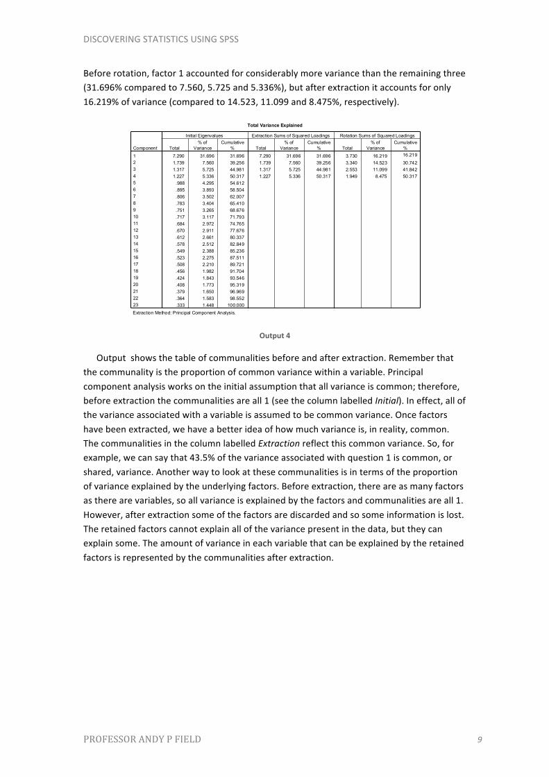
Output lists the eigenvalues associated with each linear component (factor) before extraction, after extraction and after rotation. Before extraction, SPSS has identified 23 linear components within the data set (we know that there should be as many eigenvectors as there are variables and so there will be as many factors as variables). The eigenvalues associated with each factor represent the variance explained by that particular linear component, and SPSS also displays the eigenvalue in terms of the percentage of variance explained (so factor 1 explains 31.696% of total variance). It should be clear that the first few factors explain relatively large amounts of variance (especially factor 1), whereas subsequent factors explain only small amounts of variance. SPSS then extracts all factors with eigenvalues greater than 1, which leaves us with four factors. The eigenvalues associated with these factors are again displayed (and the percentage of variance explained) in the columns labelled Extraction Sums of Squared Loadings. The values in this part of the table are the same as the values before extraction, except that the values for the discarded factors are ignored (hence, the table is blank after the fourth factor). In the final part of the table (labelled Rotation Sums of Squared Loadings), the eigenvalues of the factors after rotation are displayed. Rotation has the effect of optimizing the factor structure, and one consequence for these data is that the relative importance of the four factors is equalized.
DISCOVERING STATISTICS USING SPSS
PROFESSOR ANDY P FIELD 9
Before rotation, factor 1 accounted for considerably more variance than the remaining three (31.696% compared to 7.560, 5.725 and 5.336%), but after extraction it accounts for only 16.219% of variance (compared to 14.523, 11.099 and 8.475%, respectively).
Output 4
Output shows the table of communalities before and after extraction. Remember that the communality is the proportion of common variance within a variable. Principal component analysis works on the initial assumption that all variance is common; therefore, before extraction the communalities are all 1 (see the column labelled Initial). In effect, all of the variance associated with a variable is assumed to be common variance. Once factors have been extracted, we have a better idea of how much variance is, in reality, common. The communalities in the column labelled Extraction reflect this common variance. So, for example, we can say that 43.5% of the variance associated with question 1 is common, or shared, variance. Another way to look at these communalities is in terms of the proportion of variance explained by the underlying factors. Before extraction, there are as many factors as there are variables, so all variance is explained by the factors and communalities are all 1. However, after extraction some of the factors are discarded and so some information is lost. The retained factors cannot explain all of the variance present in the data, but they can explain some. The amount of variance in each variable that can be explained by the retained factors is represented by the communalities after extraction.
Total Variance Explained
7.290 31.696 31.696 7.290 31.696 31.696 3.730 16.219 16.219
1.739 7.560 39.256 1.739 7.560 39.256 3.340 14.523 30.7421.317 5.725 44.981 1.317 5.725 44.981 2.553 11.099 41.8421.227 5.336 50.317 1.227 5.336 50.317 1.949 8.475 50.317
.988 4.295 54.612
.895 3.893 58.504
.806 3.502 62.007
.783 3.404 65.410
.751 3.265 68.676
.717 3.117 71.793
.684 2.972 74.765
.670 2.911 77.676
.612 2.661 80.337
.578 2.512 82.849
.549 2.388 85.236
.523 2.275 87.511
.508 2.210 89.721
.456 1.982 91.704
.424 1.843 93.546
.408 1.773 95.319
.379 1.650 96.969
.364 1.583 98.552
.333 1.448 100.000
Component
1234567891011121314151617181920212223
Total% of
VarianceCumulative
% Total% of
VarianceCumulative
% Total% of
VarianceCumulative
%
Initial Eigenvalues Extraction Sums of Squared Loadings Rotation Sums of Squared Loadings
Extraction Method: Principal Component Analysis.

DISCOVERING STATISTICS USING SPSS
PROFESSOR ANDY P FIELD 10
Output 5
Output also shows the component matrix before rotation. This matrix contains the loadings of each variable onto each factor. By default SPSS displays all loadings; however, we requested that all loadings less than .4 be suppressed in the output (see Figure 6) and so there are blank spaces for many of the loadings. This matrix is not particularly important for interpretation, but it is interesting to note that before rotation most variables load highly onto the first factor.
At this stage SPSS has extracted four factors. Factor analysis is an exploratory tool and so it should be used to guide the researcher to make various decisions: you shouldn’t leave the computer to make them. One important decision is the number of factors to extract. By Kaiser’s criterion we should extract four factors and this is what SPSS has done. However, this criterion is accurate when there are less than 30 variables and communalities after extraction are greater than .7 or when the sample size exceeds 250 and the average communality is greater than .6. The communalities are shown in Output , and only one exceeds .7. The average of the communalities can be found by adding them up and dividing by the number of communalities (11.573/23 = .503). So, on both grounds Kaiser’s rule may not be accurate. However, you should consider the huge sample that we have, because the research into Kaiser’s criterion gives recommendations for much smaller samples. By Jolliffe’s criterion (retain factors with eigenvalues greater than 0.7) we should retain 10 factors, but there is little to recommend this criterion over Kaiser’s. As a final guide we can use the scree plot which we asked SPSS to produce by using the option in Figure 3. The scree plot is shown in Output . This curve is difficult to interpret because it begins to tail off after three factors, but there is another drop after four factors before a stable plateau is reached. Therefore, we could probably justify retaining either two or four factors. Given the large
Communalities
1.000 .4351.000 .4141.000 .5301.000 .4691.000 .3431.000 .6541.000 .5451.000 .7391.000 .4841.000 .3351.000 .6901.000 .5131.000 .5361.000 .4881.000 .3781.000 .4871.000 .6831.000 .5971.000 .3431.000 .4841.000 .5501.000 .4641.000 .412
Q01Q02Q03Q04Q05Q06Q07Q08Q09Q10Q11Q12Q13Q14Q15Q16Q17Q18Q19Q20Q21Q22Q23
Initial Extraction
Extraction Method: Principal Component
Component Matrixa
.701
.685
.679
.673
.669
.658
.656
.652 -.400
.643
.634 -.629 .593 .586 .556 .549 .401 -.417.437 .436 -.404
-.427 .627 .548 .465
.562 .571 .507
Q18Q07Q16Q13Q12Q21Q14Q11Q17Q04Q03Q15Q01Q05Q08Q10Q20Q19Q09Q02Q22Q06Q23
1 2 3 4Component
Extraction Method: Principal Component Analysis.4 components extracted.a.

DISCOVERING STATISTICS USING SPSS
PROFESSOR ANDY P FIELD 11
sample, it is probably safe to assume Kaiser’s criterion; however, you might like to rerun the analysis specifying that SPSS extract only two factors (see Figure 3) and compare the results.
Output 8
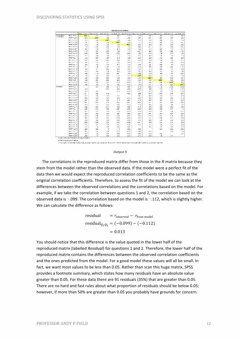
Output shows an edited version of the reproduced correlation matrix. The top half of this matrix (labelled Reproduced Correlations) contains the correlation coefficients between all of the questions based on the factor model. The diagonal of this matrix contains the communalities after extraction for each variable.
DISCOVERING STATISTICS USING SPSS
PROFESSOR ANDY P FIELD 12
Output 9
The correlations in the reproduced matrix differ from those in the R-‐matrix because they stem from the model rather than the observed data. If the model were a perfect fit of the data then we would expect the reproduced correlation coefficients to be the same as the original correlation coefficients. Therefore, to assess the fit of the model we can look at the differences between the observed correlations and the correlations based on the model. For example, if we take the correlation between questions 1 and 2, the correlation based on the observed data is −.099. The correlation based on the model is −.112, which is slightly higher. We can calculate the difference as follows:
residual = 𝑟observed − 𝑟from model
residual!!!! = −0.099 − −0.112
= 0.013
You should notice that this difference is the value quoted in the lower half of the reproduced matrix (labelled Residual) for questions 1 and 2. Therefore, the lower half of the reproduced matrix contains the differences between the observed correlation coefficients and the ones predicted from the model. For a good model these values will all be small. In fact, we want most values to be less than 0.05. Rather than scan this huge matrix, SPSS provides a footnote summary, which states how many residuals have an absolute value greater than 0.05. For these data there are 91 residuals (35%) that are greater than 0.05. There are no hard and fast rules about what proportion of residuals should be below 0.05; however, if more than 50% are greater than 0.05 you probably have grounds for concern.

DISCOVERING STATISTICS USING SPSS
PROFESSOR ANDY P FIELD 13
Orthogonal rotation (varimax)
Output shows the rotated component matrix (also called the rotated factor matrix in factor analysis), which is a matrix of the factor loadings for each variable onto each factor. This matrix contains the same information as the component matrix, except that it is calculated after rotation. There are several things to consider about the format of this matrix. First, factor loadings less than .4 have not been displayed because we asked for these loadings to be suppressed using the option in Figure 6. If you didn’t select this option, or didn’t adjust the criterion value to .4, then your output will differ. Second, the variables are listed in the order of size of their factor loadings. By default, SPSS orders the variables as they are in the data editor; however, we asked for the output to be Sorted by size using the option in Figure 6. If this option was not selected your output will look different. Finally, for all other parts of the output I suppressed the variable labels (for reasons of space), but for this matrix I have allowed the variable labels to be printed to aid interpretation.
The original logic behind suppressing loadings less than .4 was based on Stevens’ (2002) suggestion that this cut-‐off point was appropriate for interpretative purposes (i.e., loadings greater than .4 represent substantive values). However, this means that we have suppressed several loadings that are undoubtedly significant. However, significance itself is not important.
Compare this matrix to the unrotated solution (Output ). Before rotation, most variables loaded highly onto the first factor and the remaining factors didn’t really get a look in. However, the rotation of the factor structure has clarified things considerably: there are four factors and variables load very highly onto only one factor (with the exception of one question). The suppression of loadings less than .4 and ordering variables by loading size also make interpretation considerably easier (because you don’t have to scan the matrix to identify substantive loadings).
The next step is to look at the content of questions that load onto the same factor to try to identify common themes. If the mathematical factor produced by the analysis represents some real-‐world construct then common themes among highly loading questions can help us identify what the construct might be. The questions that load highly on factor 1 seem to all relate to using computers or SPSS. Therefore we might label this factor fear of computers. The questions that load highly on factor 2 all seem to relate to different aspects of statistics; therefore, we might label this factor fear of statistics. The three questions that load highly on factor 3 all seem to relate to mathematics; therefore, we might label this factor fear of mathematics. Finally, the questions that load highly on factor 4 all contain some component of social evaluation from friends; therefore, we might label this factor peer evaluation. This analysis seems to reveal that the initial questionnaire, in reality, is composed of four subscales: fear of computers, fear of statistics, fear of maths and fear of negative peer evaluation. There are two possibilities here. The first is that the SAQ failed to measure what it set out to (namely, SPSS anxiety) but does measure some related constructs. The second is that these four constructs are sub-‐components of SPSS anxiety. However, the factor analysis does not indicate which of these possibilities is true.

DISCOVERING STATISTICS USING SPSS
PROFESSOR ANDY P FIELD 14
Output 8
The final part of the output is the factor transformation matrix. This matrix provides information about the degree to which the factors were rotated to obtain a solution. If no rotation were necessary, this matrix would be an identity matrix. If orthogonal rotation were completely appropriate then we would expect a symmetrical matrix (same values above and below the diagonal). In reality the matrix is not easy to interpret, although very asymmetrical matrices might be taken as a reason to try oblique rotation. For the inexperienced factor analyst you are probably best advised to ignore the factor transformation matrix.
Rotated Component Matrixa
.800
.684
.647
.638
.579
.550
.459 .677
.661
-.567
.473 .523
.516
.514 .496 .429 .833 .747 .747 .648 .645 .586
.543
.427
I have little experience of computersSPSS always crashes when I try to use itI worry that I will cause irreparable damage becauseof my incompetenece with computersAll computers hate meComputers have minds of their own and deliberatelygo wrong whenever I use themComputers are useful only for playing gamesComputers are out to get meI can't sleep for thoughts of eigen vectorsI wake up under my duvet thinking that I am trappedunder a normal distribtionStandard deviations excite mePeople try to tell you that SPSS makes statisticseasier to understand but it doesn'tI dream that Pearson is attacking me with correlationcoefficientsI weep openly at the mention of central tendencyStatiscs makes me cryI don't understand statisticsI have never been good at mathematicsI slip into a coma whenever I see an equationI did badly at mathematics at schoolMy friends are better at statistics than meMy friends are better at SPSS than I amIf I'm good at statistics my friends will think I'm a nerdMy friends will think I'm stupid for not being able tocope with SPSSEverybody looks at me when I use SPSS
1 2 3 4Component
Extraction Method: Principal Component Analysis. Rotation Method: Varimax with Kaiser Normalization.
Rotation converged in 9 iterations.a.
Component Transformation Matrix
.635 .585 .443 -.242
.137 -.168 .488 .846
.758 -.513 -.403 .008
.067 .605 -.635 .476
Component
1234
1 2 3 4
Extraction Method: Principal Component Analysis. Rotation Method: Varimax with Kaiser Normalization.
DISCOVERING STATISTICS USING SPSS
PROFESSOR ANDY P FIELD 15
Oblique rotation
Output 9
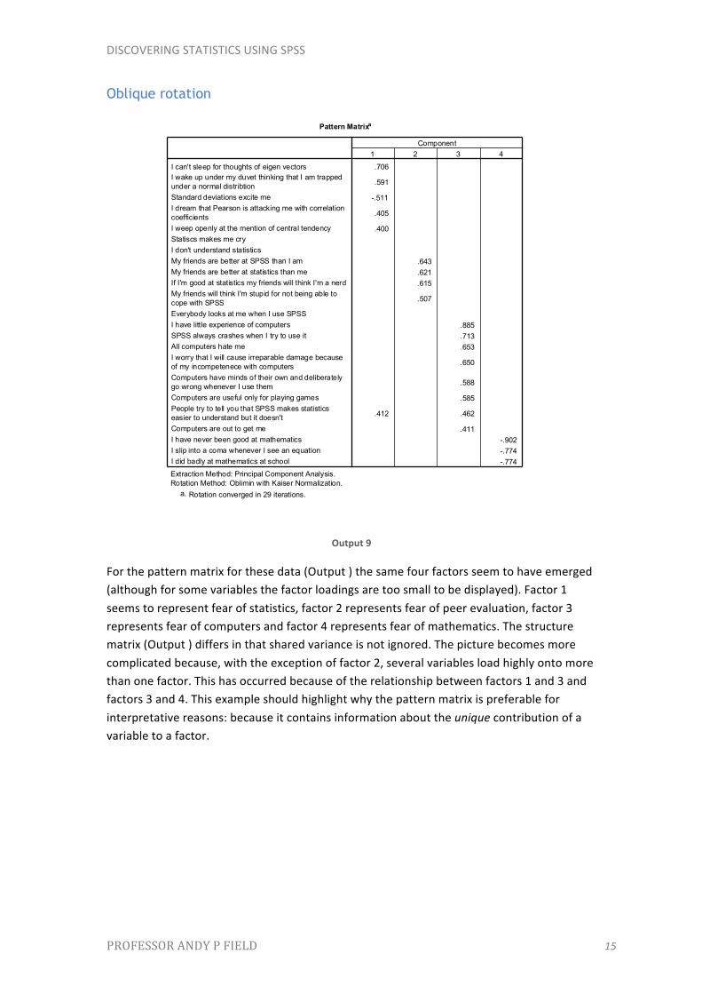
For the pattern matrix for these data (Output ) the same four factors seem to have emerged (although for some variables the factor loadings are too small to be displayed). Factor 1 seems to represent fear of statistics, factor 2 represents fear of peer evaluation, factor 3 represents fear of computers and factor 4 represents fear of mathematics. The structure matrix (Output ) differs in that shared variance is not ignored. The picture becomes more complicated because, with the exception of factor 2, several variables load highly onto more than one factor. This has occurred because of the relationship between factors 1 and 3 and factors 3 and 4. This example should highlight why the pattern matrix is preferable for interpretative reasons: because it contains information about the unique contribution of a variable to a factor.
Pattern Matrixa
.706
.591
-.511
.405
.400 .643 .621 .615
.507
.885 .713 .653
.650
.588
.585
.412 .462
.411 -.902 -.774 -.774
I can't sleep for thoughts of eigen vectorsI wake up under my duvet thinking that I am trappedunder a normal distribtionStandard deviations excite meI dream that Pearson is attacking me with correlationcoefficientsI weep openly at the mention of central tendencyStatiscs makes me cryI don't understand statisticsMy friends are better at SPSS than I amMy friends are better at statistics than meIf I'm good at statistics my friends will think I'm a nerdMy friends will think I'm stupid for not being able tocope with SPSSEverybody looks at me when I use SPSSI have little experience of computersSPSS always crashes when I try to use itAll computers hate meI worry that I will cause irreparable damage becauseof my incompetenece with computersComputers have minds of their own and deliberatelygo wrong whenever I use themComputers are useful only for playing gamesPeople try to tell you that SPSS makes statisticseasier to understand but it doesn'tComputers are out to get meI have never been good at mathematicsI slip into a coma whenever I see an equationI did badly at mathematics at school
1 2 3 4Component
Extraction Method: Principal Component Analysis. Rotation Method: Oblimin with Kaiser Normalization.
Rotation converged in 29 iterations.a.

DISCOVERING STATISTICS USING SPSS
PROFESSOR ANDY P FIELD 16
Output 1
The final part of the output is a correlation matrix between the factors (Output ). This matrix contains the correlation coefficients between factors. As predicted from the structure matrix, factor 2 has little or no relationship with any other factors (correlation coefficients are low), but all other factors are interrelated to some degree (notably factors 1 and 3 and factors 3 and 4). The fact that these correlations exist tell us that the constructs measured can be interrelated. If the constructs were independent then we would expect oblique rotation to provide an identical solution to an orthogonal rotation and the component correlation matrix should be an identity matrix (i.e., all factors have correlation coefficients of 0). Therefore, this final matrix gives us a guide to whether it is reasonable to assume independence between factors: for these data it appears that we cannot assume independence. Therefore, the results of the orthogonal rotation should not be trusted: the obliquely rotated solution is probably more meaningful.
On a theoretical level the dependence between our factors does not cause concern; we might expect a fairly strong relationship between fear of maths, fear of statistics and fear of computers. Generally, the less mathematically and technically minded people struggle with statistics. However, we would not expect these constructs to correlate with fear of peer evaluation (because this construct is more socially based). In fact, this factor is the one that correlates fairly badly with all others – so on a theoretical level, things have turned out rather well!
Structure Matrix
.695 .477
.685 -.632 -.407 .567 .516 -.491
.548 .487 -.485
.520 .413 -.501
.462 .453 .660 .653 .588
.546
-.435 .446 .777
.404 .761
.401 .723
.723 -.429
.426 .671
.576 .606
.561 -.441 .556 -.855 .453 -.822 .451 -.818
I wake up under my duvet thinking that I am trapped undera normal distribtionI can't sleep for thoughts of eigen vectorsStandard deviations excite meI weep openly at the mention of central tendencyI dream that Pearson is attacking me with correlationcoefficientsStatiscs makes me cryI don't understand statisticsMy friends are better at SPSS than I amMy friends are better at statistics than meIf I'm good at statistics my friends will think I'm a nerdMy friends will think I'm stupid for not being able to copewith SPSSEverybody looks at me when I use SPSSI have little experience of computersSPSS always crashes when I try to use itAll computers hate meI worry that I will cause irreparable damage because ofmy incompetenece with computersComputers have minds of their own and deliberately gowrong whenever I use themPeople try to tell you that SPSS makes statistics easier tounderstand but it doesn'tComputers are out to get meComputers are useful only for playing gamesI have never been good at mathematicsI slip into a coma whenever I see an equationI did badly at mathematics at school
1 2 3 4Component
Extraction Method: Principal Component Analysis. Rotation Method: Oblimin with Kaiser Normalization.

DISCOVERING STATISTICS USING SPSS
PROFESSOR ANDY P FIELD 17
Output 2
Factor scores
Having reached a suitable solution and rotated that solution, we can look at the factor scores. Output shows the component score matrix B from which the factor scores are calculated and the covariance matrix of factor scores. The component score matrix is not particularly useful in itself. It can be useful in understanding how the factor scores have been computed, but with large data sets like this one you are unlikely to want to delve into the mathematics behind the factor scores. However, the covariance matrix of scores is useful. This matrix in effect tells us the relationship between factor scores (it is an unstandardized correlation matrix). If factor scores are uncorrelated then this matrix should be an identity matrix (i.e., diagonal elements will be 1 but all other elements are 0). For these data the covariances are all zero, indicating that the resulting scores are uncorrelated.
Component Correlation Matrix
1.000 -.154 .364 -.279-.154 1.000 -.185 8.155E-02.364 -.185 1.000 -.464
-.279 8.155E-02 -.464 1.000
Component1234
1 2 3 4
Extraction Method: Principal Component Analysis. Rotation Method: Oblimin with Kaiser Normalization.

DISCOVERING STATISTICS USING SPSS
PROFESSOR ANDY P FIELD 18
Output 3
In the original analysis we asked for scores to be calculated based on the Anderson–Rubin method (hence why they are uncorrelated). You will find these scores in the data editor. There should be four new columns of data (one for each factor) labelled FAC1_1, FAC2_1, FAC3_1 and FAC4_1 respectively. If you asked for factor scores in the oblique rotation then these scores will appear in the data editor in four other columns labelled FAC2_1 and so on.
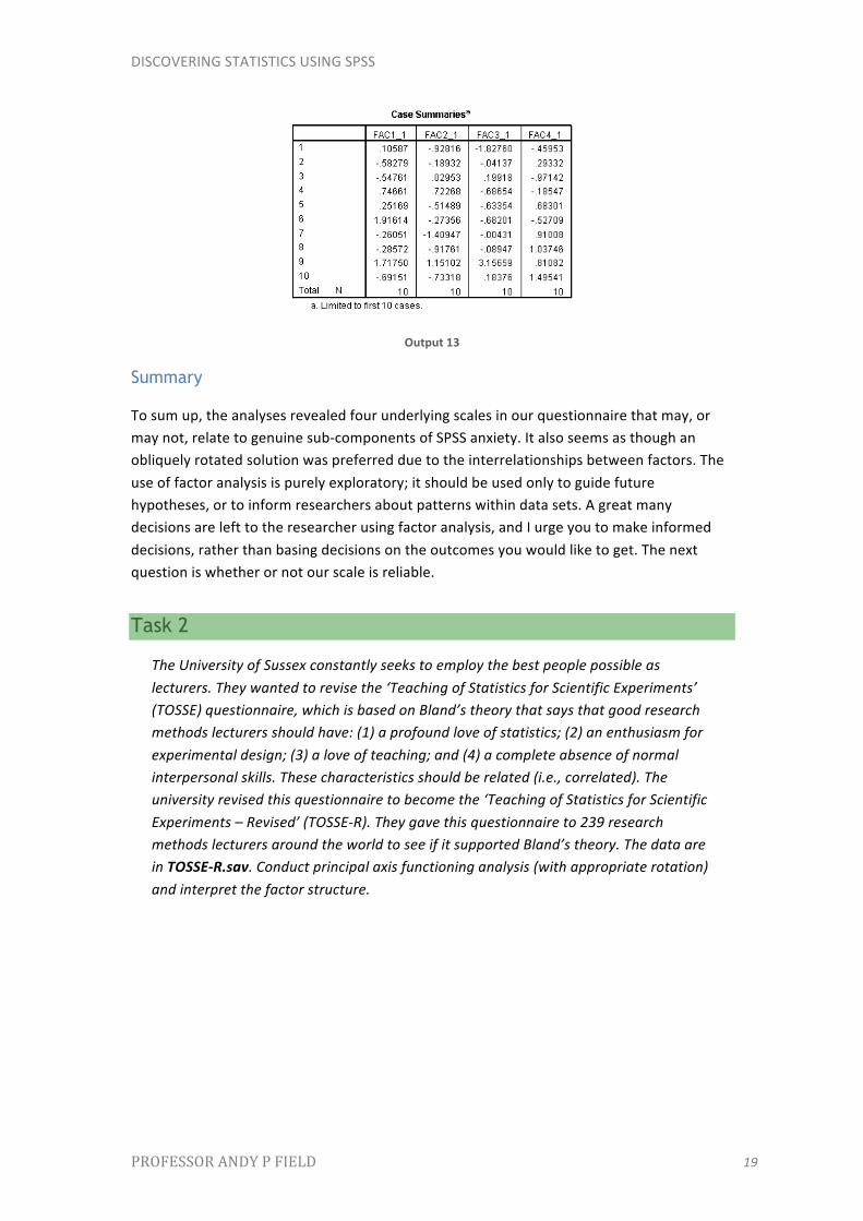
Output shows the factor scores for the first 10 participants. It should be pretty clear that participant 9 scored highly on all four factors, and so this person is very anxious about statistics, computing and maths, but less so about peer evaluation (factor 4). Factor scores can be used in this way to assess the relative fear of one person compared to another, or we could add the scores up to obtain a single score for each participant (that we might assume represents SPSS anxiety as a whole). We can also use factor scores in regression when groups of predictors correlate so highly that there is multicollinearity.
DISCOVERING STATISTICS USING SPSS
PROFESSOR ANDY P FIELD 19
Output 13
Summary
To sum up, the analyses revealed four underlying scales in our questionnaire that may, or may not, relate to genuine sub-‐components of SPSS anxiety. It also seems as though an obliquely rotated solution was preferred due to the interrelationships between factors. The use of factor analysis is purely exploratory; it should be used only to guide future hypotheses, or to inform researchers about patterns within data sets. A great many decisions are left to the researcher using factor analysis, and I urge you to make informed decisions, rather than basing decisions on the outcomes you would like to get. The next question is whether or not our scale is reliable.
Task 2
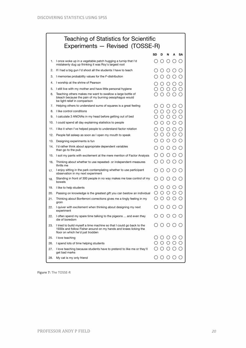
The University of Sussex constantly seeks to employ the best people possible as lecturers. They wanted to revise the ‘Teaching of Statistics for Scientific Experiments’ (TOSSE) questionnaire, which is based on Bland’s theory that says that good research methods lecturers should have: (1) a profound love of statistics; (2) an enthusiasm for experimental design; (3) a love of teaching; and (4) a complete absence of normal interpersonal skills. These characteristics should be related (i.e., correlated). The university revised this questionnaire to become the ‘Teaching of Statistics for Scientific Experiments – Revised’ (TOSSE-‐R). They gave this questionnaire to 239 research methods lecturers around the world to see if it supported Bland’s theory. The data are in TOSSE-‐R.sav. Conduct principal axis functioning analysis (with appropriate rotation) and interpret the factor structure.
DISCOVERING STATISTICS USING SPSS
PROFESSOR ANDY P FIELD 20
Figure 7: The TOSSE-‐R
I once woke up in a vegetable patch hugging a turnip that I'd mistakenly dug up thinking it was Roy's largest root
If I had a big gun I'd shoot all the students I have to teach
I memorise probability values for the F-distribution
I worship at the shrine of Pearson
I still live with my mother and have little personal hygieneTeaching others makes me want to swallow a large bottle of bleach because the pain of my burning oesophagus would be light relief in comparison
I like control conditions
Helping others to understand sums of squares is a great feeling
I could spend all day explaining statistics to people
I calculate 3 ANOVAs in my head before getting out of bed
People fall asleep as soon as I open my mouth to speak
I like it when I've helped people to understand factor rotation
Designing experiments is funI'd rather think about appropriate dependent variables than go to the pub
I soil my pants with excitement at the mere mention of Factor Analysis
Thinking about whether to use repeated- or independent-measures thrills meI enjoy sitting in the park contemplating whether to use participant observation in my next experiment
1.
2.
3.
4.
5.6.
7.8.9.
10.
11.
12.
13.14.
15.
16.
17.
SD D N A SA
Teaching of Statistics for Scientific Experiments — Revised (TOSSE-R)
Standing in front of 300 people in no way makes me lose control of my bowels
18.
I like to help students19.
Passing on knowledge is the greatest gift you can bestow an individual20.
Thinking about Bonferroni corrections gives me a tingly feeling in my groin
21.
I quiver with excitement when thinking about designing my next experiment
22.
I often spend my spare time talking to the pigeons ... and even they die of boredom
22.
I tried to build myself a time machine so that I could go back to the 1930s and follow Fisher around on my hands and knees licking the floor on which he'd just trodden
23.
I love teaching25.
I spend lots of time helping students26.
I love teaching because students have to pretend to like me or they'll get bad marks
27.
My cat is my only friend28.

DISCOVERING STATISTICS USING SPSS
PROFESSOR ANDY P FIELD 21
Multicollinearity. The determinant of the correlation matrix was .00000124, which is smaller than .00001 and, therefore, indicates that multicollinearity could be a problem in these data (although, strictly speaking, because we’re using principal component analysis we don’t need to worry).
Output 14
Output 15

DISCOVERING STATISTICS USING SPSS
PROFESSOR ANDY P FIELD 22
Sample size. MacCallum et al. (1999) have demonstrated that when communalities after extraction are above .5 a sample size between 100 and 200 can be adequate, and even when communalities are below .5 a sample size of 500 should be sufficient. We have a sample size of 239 with some communalities below .5, and so the sample size may not be adequate. However, the KMO measure of sampling adequacy is .894, which is above Kaiser’s (1974) recommendation of .5. This value is also ‘meritorious’ (and almost ‘marvellous’) according to Hutcheson and Sofroniou (1999). As such, the evidence suggests that the sample size is adequate to yield distinct and reliable factors.
Bartlett’s test. This tests whether the correlations between questions are sufficiently large for factor analysis to be appropriate (it actually tests whether the correlation matrix is sufficiently different from an identity matrix). In this case it is significant, χ2(378) = 2989.77, p < .001, indicating that the correlations within the R-‐matrix are sufficiently different from zero to warrant factor analysis.

DISCOVERING STATISTICS USING SPSS
PROFESSOR ANDY P FIELD 23
Output 16

DISCOVERING STATISTICS USING SPSS
PROFESSOR ANDY P FIELD 24
Output 17
Extraction: SPSS has extracted five factors based on Kaiser’s criterion of retaining factors with eigenvalues greater than 1. Is this warranted? Kaiser’s criterion is accurate when there are less than 30 variables and the communalities after extraction are greater than .7, or when the sample size exceeds 250 and the average communality is greater than .6. For these data the sample size is 239, there are 28 variables, and the mean communality is .488, so extracting five factors is not really warranted. The scree plot shows clear inflexions at 3 and 5 factors and so using the scree plot you could justify extracting 3 or 5 factors.
DISCOVERING STATISTICS USING SPSS
PROFESSOR ANDY P FIELD 25
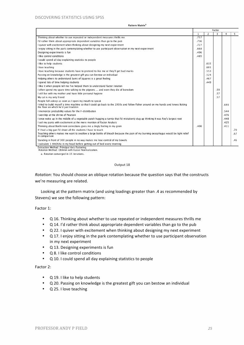
Output 18
Rotation: You should choose an oblique rotation because the question says that the constructs we’re measuring are related.
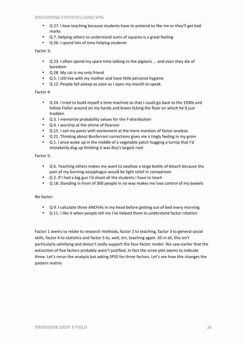
Looking at the pattern matrix (and using loadings greater than .4 as recommended by Stevens) we see the following pattern:
Factor 1:
• Q 16. Thinking about whether to use repeated or independent measures thrills me • Q 14. I’d rather think about appropriate dependent variables than go to the pub • Q 22. I quiver with excitement when thinking about designing my next experiment • Q 17. I enjoy sitting in the park contemplating whether to use participant observation
in my next experiment • Q 13. Designing experiments is fun • Q 8. I like control conditions • Q 10. I could spend all day explaining statistics to people
Factor 2:
• Q 19. I like to help students • Q 20. Passing on knowledge is the greatest gift you can bestow an individual • Q 25. I love teaching
DISCOVERING STATISTICS USING SPSS
PROFESSOR ANDY P FIELD 26
• Q 27. I love teaching because students have to pretend to like me or they’ll get bad marks
• Q 7. Helping others to understand sums of squares is a great feeling • Q 26. I spend lots of time helping students
Factor 3:
• Q 23. I often spend my spare time talking to the pigeons ... and even they die of boredom
• Q 28. My cat is my only friend • Q 5. I still live with my mother and have little personal hygiene • Q 12. People fall asleep as soon as I open my mouth to speak
Factor 4:
• Q 24. I tried to build myself a time machine so that I could go back to the 1930s and follow Fisher around on my hands and knees licking the floor on which he’d just trodden
• Q 3. I memorize probability values for the F-‐distribution • Q 4. I worship at the shrine of Pearson • Q 15. I soil my pants with excitement at the mere mention of factor analysis • Q 21. Thinking about Bonferroni corrections gives me a tingly feeling in my groin • Q 1. I once woke up in the middle of a vegetable patch hugging a turnip that I’d
mistakenly dug up thinking it was Roy’s largest root
Factor 5:
• Q 6. Teaching others makes me want to swallow a large bottle of bleach because the pain of my burning oesophagus would be light relief in comparison
• Q 2. If I had a big gun I’d shoot all the students I have to teach • Q 18. Standing in front of 300 people in no way makes me lose control of my bowels
No factor:
• Q 9. I calculate three ANOVAs in my head before getting out of bed every morning • Q 11. I like it when people tell me I’ve helped them to understand factor rotation
Factor 1 seems to relate to research methods, factor 2 to teaching, factor 3 to general social skills, factor 4 to statistics and factor 5 to, well, err, teaching again. All in all, this isn’t particularly satisfying and doesn’t really support the four-‐factor model. We saw earlier that the extraction of five factors probably wasn’t justified. In fact the scree plot seems to indicate three. Let’s rerun the analysis but asking SPSS for three factors. Let’s see how this changes the pattern matrix:
DISCOVERING STATISTICS USING SPSS
PROFESSOR ANDY P FIELD 27
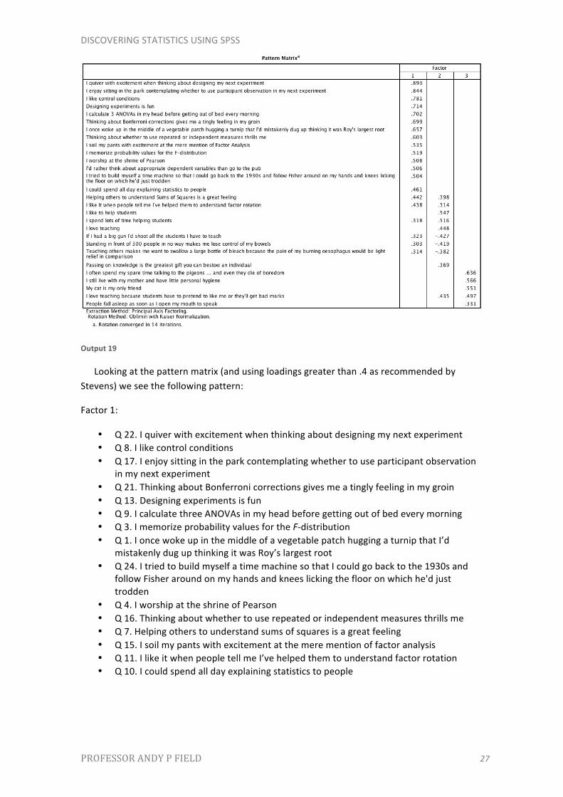
Output 19
Looking at the pattern matrix (and using loadings greater than .4 as recommended by Stevens) we see the following pattern:
Factor 1:
• Q 22. I quiver with excitement when thinking about designing my next experiment • Q 8. I like control conditions • Q 17. I enjoy sitting in the park contemplating whether to use participant observation
in my next experiment • Q 21. Thinking about Bonferroni corrections gives me a tingly feeling in my groin • Q 13. Designing experiments is fun • Q 9. I calculate three ANOVAs in my head before getting out of bed every morning • Q 3. I memorize probability values for the F-‐distribution • Q 1. I once woke up in the middle of a vegetable patch hugging a turnip that I’d
mistakenly dug up thinking it was Roy’s largest root • Q 24. I tried to build myself a time machine so that I could go back to the 1930s and
follow Fisher around on my hands and knees licking the floor on which he'd just trodden
• Q 4. I worship at the shrine of Pearson • Q 16. Thinking about whether to use repeated or independent measures thrills me • Q 7. Helping others to understand sums of squares is a great feeling • Q 15. I soil my pants with excitement at the mere mention of factor analysis • Q 11. I like it when people tell me I’ve helped them to understand factor rotation • Q 10. I could spend all day explaining statistics to people

DISCOVERING STATISTICS USING SPSS
PROFESSOR ANDY P FIELD 28
• Q 14. I’d rather think about appropriate dependent variables than go to the pub
Factor 2:
• Q 19. I like to help students • Q 2. If I had a big gun I’d shoot all the students I have to teach (note negative weight) • Q 6. Teaching others makes me want to swallow a large bottle of bleach because the
pain of my burning oesophagus would be light relief in comparison (note negative weight)
• Q 18. Standing in front of 300 people in no way makes me lose control of my bowels (note negative weight)
• Q 26. I spend lots of time helping students • Q 25. I love teaching • Q 20. Passing on knowledge is the greatest gift you can bestow an individual
Factor 3:
• Q 5. I still live with my mother and have little personal hygiene • Q 23. I often spend my spare time talking to the pigeons ... and even they die of
boredom • Q 28. My cat is my only friend • Q 12. People fall asleep as soon as I open my mouth to speak • Q 27. I love teaching because students have to pretend to like me or they’ll get bad
marks
This factor is a lot clearer-‐cut: factor 1 relates to a love of methods and statistics, factor 2 to a love of teaching, and factor 3 to an absence of normal social skills. This doesn’t support the original four-‐factor model suggested because the data indicate that love of methods and statistics can’t be separated (if you love one you love the other).
Task 3
Dr Sian Williams (University of Brighton) devised a questionnaire to measure organizational ability. She predicted five factors to do with organizational ability: (1) preference for organization; (2) goal achievement; (3) planning approach; (4) acceptance of delays; and (5) preference for routine. These dimensions are theoretically independent. Williams’ questionnaire contains 28 items using a 7-‐point Likert scale (1 = strongly disagree, 4 = neither, 7 = strongly agree). She gave it to 239 people. Run a principal component analysis on the data in Williams.sav.
1 I like to have a plan to work to in everyday life
2 I feel frustrated when things don’t go to plan
3 I get most things done in a day that I want to
4 I stick to a plan once I have made it
5 I enjoy spontaneity and uncertainty
6 I feel frustrated if I can’t find something I need

DISCOVERING STATISTICS USING SPSS
PROFESSOR ANDY P FIELD 29
7 I find it difficult to follow a plan through
8 I am an organized person
9 I like to know what I have to do in a day
10 Disorganized people annoy me
11 I leave things to the last minute
12 I have many different plans relating to the same goal
13 I like to have my documents filed and in order 14 I find it easy to work in a disorganized environment 15 I make ‘to do’ lists and achieve most of the things on it
16 My workspace is messy and disorganized
17 I like to be organized
18 Interruptions to my daily routine annoy me
19 I feel that I am wasting my time
20 I forget the plans I have made
21 I prioritize the things I have to do
22 I like to work in an organized environment
23 I feel relaxed when I don't have a routine
24 I set deadlines for myself and achieve them
25 I change rather aimlessly from one activity to another during the day
26 I have trouble organizing the things I have to do
27 I put tasks off to another day
28 I feel restricted by schedules and plans
Output 4
Output 5
KMO and Bartlett's Test
.894
2989.769378.000
Kaiser-Meyer-Olkin Measure of SamplingAdequacy.
Approx. Chi-SquaredfSig.
Bartlett's Test ofSphericity
DISCOVERING STATISTICS USING SPSS
PROFESSOR ANDY P FIELD 30
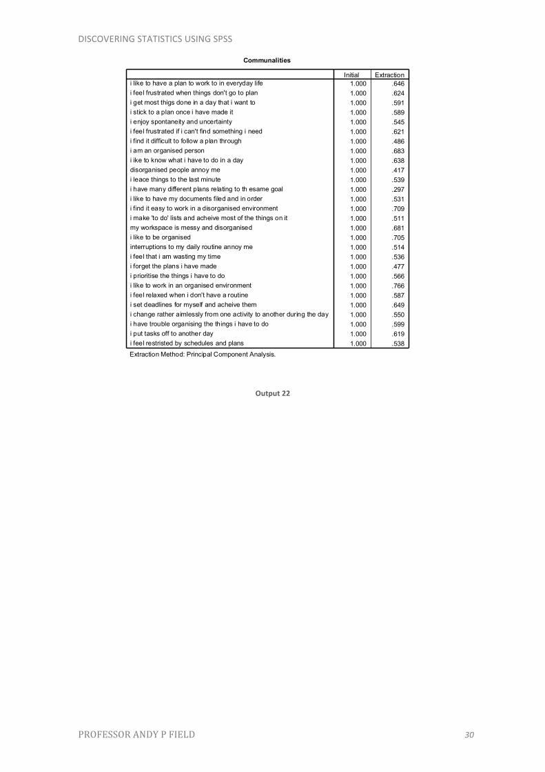
Output 22
Communalities
1.000 .6461.000 .6241.000 .5911.000 .5891.000 .5451.000 .6211.000 .4861.000 .6831.000 .6381.000 .4171.000 .5391.000 .2971.000 .5311.000 .7091.000 .5111.000 .6811.000 .7051.000 .5141.000 .5361.000 .4771.000 .5661.000 .7661.000 .5871.000 .6491.000 .5501.000 .5991.000 .6191.000 .538
i like to have a plan to work to in everyday lifei feel frustrated when things don't go to plani get most thigs done in a day that i want toi stick to a plan once i have made iti enjoy spontaneity and uncertaintyi feel frustrated if i can't find something i needi find it difficult to follow a plan throughi am an organised personi ike to know what i have to do in a daydisorganised people annoy mei leace things to the last minutei have many different plans relating to th esame goali like to have my documents filed and in orderi find it easy to work in a disorganised environmenti make 'to do' lists and acheive most of the things on itmy workspace is messy and disorganisedi like to be organisedinterruptions to my daily routine annoy mei feel that i am wasting my timei forget the plans i have madei prioritise the things i have to doi like to work in an organised environmenti feel relaxed when i don't have a routinei set deadlines for myself and acheive themi change rather aimlessly from one activity to another during the dayi have trouble organising the things i have to doi put tasks off to another dayi feel restristed by schedules and plans
Initial Extraction
Extraction Method: Principal Component Analysis.

DISCOVERING STATISTICS USING SPSS
PROFESSOR ANDY P FIELD 31
Output 23
Output 24
Total Variance Explained
9.064 32.373 32.373 9.064 32.373 32.373 4.558 16.279 16.2792.787 9.954 42.328 2.787 9.954 42.328 3.460 12.356 28.6351.664 5.944 48.272 1.664 5.944 48.272 3.239 11.568 40.2031.515 5.409 53.681 1.515 5.409 53.681 2.631 9.397 49.6001.180 4.215 57.896 1.180 4.215 57.896 2.323 8.296 57.896
.991 3.539 61.435
.925 3.304 64.739
.819 2.924 67.663
.793 2.832 70.495
.744 2.657 73.152
.705 2.518 75.670
.654 2.336 78.005
.623 2.224 80.229
.574 2.051 82.281
.545 1.945 84.225
.516 1.841 86.067
.487 1.740 87.806
.454 1.621 89.427
.423 1.511 90.938
.382 1.363 92.301
.341 1.218 93.519
.334 1.193 94.712
.309 1.102 95.814
.293 1.046 96.860
.260 .928 97.788
.248 .887 98.675
.207 .738 99.414
.164 .586 100.000
Component12345678910111213141516171819202122232425262728
Total % of Variance Cumulative % Total % of Variance Cumulative % Total % of Variance Cumulative %Initial Eigenvalues Extraction Sums of Squared Loadings Rotation Sums of Squared Loadings
Extraction Method: Principal Component Analysis.

DISCOVERING STATISTICS USING SPSS
PROFESSOR ANDY P FIELD 32
Output 25
Component Matrixa
.684 -.543
.584
.600 .452
.446 .524 -.501 .453
.528
.803
.723
.502
.675 .519
.673
.614 -.517
.559
.650 -.497
.768
.421 -.523 .620
.456
.674
.791
.432 .518
.614
.501 .444
.533 .502
.580
.458 .520
i like to have a plan to work to in everyday lifei feel frustrated when things don't go to plani get most thigs done in a day that i want toi stick to a plan once i have made iti enjoy spontaneity and uncertaintyi feel frustrated if i can't find something i needi find it difficult to follow a plan throughi am an organised personi ike to know what i have to do in a daydisorganised people annoy mei leace things to the last minutei have many different plans relating to th esame goali like to have my documents filed and in orderi find it easy to work in a disorganised environmenti make 'to do' lists and acheive most of the things on itmy workspace is messy and disorganisedi like to be organisedinterruptions to my daily routine annoy mei feel that i am wasting my timei forget the plans i have madei prioritise the things i have to doi like to work in an organised environmenti feel relaxed when i don't have a routinei set deadlines for myself and acheive themi change rather aimlessly from one activity to another during the dayi have trouble organising the things i have to doi put tasks off to another dayi feel restristed by schedules and plans
1 2 3 4 5Component
Extraction Method: Principal Component Analysis.5 components extracted.a.

DISCOVERING STATISTICS USING SPSS
PROFESSOR ANDY P FIELD 33
Output 26
Output 27
Extraction. SPSS has extracted five factors based on Kaiser’s criterion of retaining factors with eigenvalues greater than 1. Is this warranted? Kaiser’s criterion is accurate when there are less than 30 variables and the communalities after extraction are greater than .7, or when the sample size exceeds 250 and the average communality is greater than .6. For these data the sample size is 239 and the mean communality is .579, so extracting five factors is not really warranted. The scree plot shows clear inflexions at 3 and 5 factors, and so using the scree plot you could justify extracting 3 or 5 factors.
Rotated Component Matrixa
.409 .545 .765 .666 .619 .666 .781 .535
.587
.432 .470 .447
.440 .450 .435 .506
.593
.764
.447 .509
.775
.714 .586 .712 .649
.505 .523
.748 .672 .744 .688
.407 .568 .613 .411 .673
i like to have a plan to work to in everyday lifei feel frustrated when things don't go to plani get most thigs done in a day that i want toi stick to a plan once i have made iti enjoy spontaneity and uncertaintyi feel frustrated if i can't find something i needi find it difficult to follow a plan throughi am an organised personi ike to know what i have to do in a daydisorganised people annoy mei leace things to the last minutei have many different plans relating to th esame goali like to have my documents filed and in orderi find it easy to work in a disorganised environmenti make 'to do' lists and acheive most of the things on itmy workspace is messy and disorganisedi like to be organisedinterruptions to my daily routine annoy mei feel that i am wasting my timei forget the plans i have madei prioritise the things i have to doi like to work in an organised environmenti feel relaxed when i don't have a routinei set deadlines for myself and acheive themi change rather aimlessly from one activity to another during the dayi have trouble organising the things i have to doi put tasks off to another dayi feel restristed by schedules and plans
1 2 3 4 5Component
Extraction Method: Principal Component Analysis. Rotation Method: Varimax with Kaiser Normalization.
Rotation converged in 7 iterations.a.
Component Transformation Matrix
.633 .520 .384 .302 .301-.118 .050 .738 -.650 -.129-.188 -.346 .106 -.053 .911-.742 .503 .201 .393 .038.025 -.595 .506 .574 -.246
Component12345
1 2 3 4 5
Extraction Method: Principal Component Analysis. Rotation Method: Varimax with Kaiser Normalization.

DISCOVERING STATISTICS USING SPSS
PROFESSOR ANDY P FIELD 34
Looking at the rotated component matrix (and using loadings greater than .4 as recommended by Stevens) we see the following pattern:
Factor 1: preference for organization
• Q8: I am an organized person • Q13: I like to have my documents filed and in order • Q14: I find it easy to work in a disorganized environment • Q 16: My workspace is messy and disorganized • Q17: I like to be organized • Q22: I like to work in an organized environment
Note: It’s odd that none of these have reverse loadings.
Factor 2: plan approach
• Q1: I like to have a plan to work to in everyday life • Q3: I get most things done in a day that I want to • Q4: I stick to a plan once I have made it • Q9: I like to know what I have to do in a day • Q15: I make ‘to do’ lists and achieve most of the things on it • Q 21: I prioritize the things I have to do • Q24: I set deadlines for myself and achieve them
Factor 3: goal achievement
• Q7: I find it difficult to follow a plan through • Q11: I leave things to the last minute • Q19: I feel that I am wasting my time • Q20: I forget the plans I have made • Q25: I change rather aimlessly from one activity to another during the day • Q26: I have trouble organizing the things I have to do • Q27: I put tasks off to another day
Factor 4: acceptance of delays
• Q2: I feel frustrated when things don’t go to plan • Q6: I feel frustrated if I can’t find something I need • Q10: Disorganized people annoy me • Q18: Interruptions to my daily routine annoy me
Factor 5: preference for routine
• Q5: I enjoy spontaneity and uncertainty • Q12: I have many different plans relating to the same goal • Q23: I feel relaxed when I don't have a routine
DISCOVERING STATISTICS USING SPSS
PROFESSOR ANDY P FIELD 35
• Q28: I feel restricted by schedules and plans
Therefore, it seems as though there is some factorial validity to the structure.
Task 4
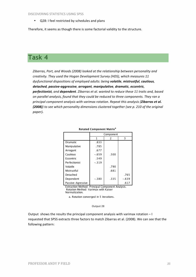
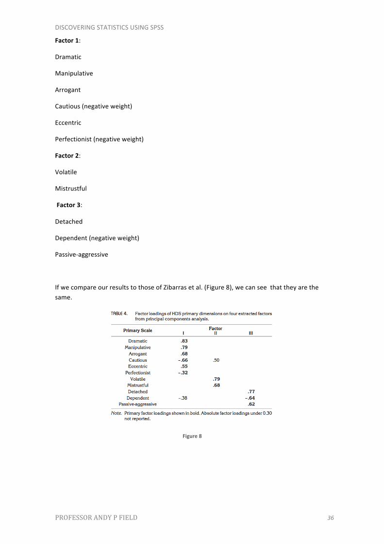
Zibarras, Port, and Woods (2008) looked at the relationship between personality and creativity. They used the Hogan Development Survey (HDS), which measures 11 dysfunctional dispositions of employed adults: being volatile, mistrustful, cautious, detached, passive-‐aggressive, arrogant, manipulative, dramatic, eccentric, perfectionist, and dependent. Zibarras et al. wanted to reduce these 11 traits and, based on parallel analysis, found that they could be reduced to three components. They ran a principal component analysis with varimax rotation. Repeat this analysis (Zibarras et al. (2008)) to see which personality dimensions clustered together (see p. 210 of the original paper).
Output 28
Output shows the results the principal component analysis with varimax rotation – I requested that SPSS extracts three factors to match Zibarras et al. (2008). We can see that the following pattern:
DISCOVERING STATISTICS USING SPSS
PROFESSOR ANDY P FIELD 36
Factor 1:
Dramatic
Manipulative
Arrogant
Cautious (negative weight)
Eccentric
Perfectionist (negative weight)
Factor 2:
Volatile
Mistrustful
Factor 3:
Detached
Dependent (negative weight)
Passive-‐aggressive
If we compare our results to those of Zibarras et al. (Figure 8), we can see that they are the same.
Figure 8