chapter 16: ground acceleration matlab model from ansys...

CHAPTER 16

GROUND ACCELERATION MATLAB MODEL FROM ANSYS MODEL

16.1 Introduction

This chapter will continue to explore building MATLAB state space models from ANSYS finite element results. We will use a different cantilever model, where the cantilever has an additional tip mass and a tip spring all mounted on a “shaker” base. This model will be a crude approximation of understanding the effects of disk drive suspension resonances on undesired unloading of the recording head during external vibration events. The problem shows how to model ground acceleration forcing functions using ANSYS and MATLAB. We will also see how to do sorting of modes in the presence of a rigid body mode. In addition, there is a high frequency mode of the system with a large dc gain, meaning that if unsorted modal truncation were used to decrease the model size, the resulting model would have significant error.

16.2 Model Description

Shaker Mass

Shaker Motion

Cantilever Beam

Beam Tip Mass

Spring

Z

X

Figure 16.1: Ground displacement model for cantilever with tip mass and tip spring.

The figure above shows a schematic of the system to be analyzed. Once again, the cantilever is a 2mm wide by 0.075mm thick by 20mm long steel beam. At the tip, a lumped mass of 0.00002349 Kg is attached. The tip mass was arbitrarily chosen to have the same mass as the beam. The spring attaching the

© 2001 by Chapman & Hall/CRC

beam tip to the shaker has a stiffness of 1e6 mN/mm. The 0.05 Kg shaker mass was chosen to be approximately 1000 times the mass of the beam and tip mass combination, making the motions of the shaker insensitive to resonances of the beam. Thus, we can apply forces to the shaker and excite it to a known acceleration amplitude. This amplitude will then be transmitted to the base of the cantilever and the shaker attachment for the beam tip spring – effectively imparting a “ground acceleration” of any desired amplitude and shape to the flexible system. Of course, since the shaker body is not constrained, it will have large rigid body movements, but we are interested in the difference between the shaker motion and the motion of the tip, so we can ignore the rigid body motion.

In a disk drive, the cantilever would represent the “suspension,” the small sheet metal device which supports the recording head, represented by the beam tip mass. The recording head is typically preloaded onto the disk with several grams of loading force by pre-bending and then displacing the suspension. This loading force is required to counteract the force generated by the air bearing when the disk is spinning, keeping the recording head a controlled distance from the disk and allowing efficient magnetic recording. During transportation of the disk drive it is subject to vibration and shock events in the z direction as indicated by the Shaker Motion arrow. Of course, vibration and shock occur in all directions, but the z direction is the most sensitive. In the z direction, the vibration or shock event may be large enough and have frequency content which will excite the suspension resonances, generating unloading forces at the head that could cause it to become momentarily unloaded. When unloaded, the slider will re-approach the disk and possibly damage the disk. Thus, understanding resonant characteristics of the suspension and the resulting tendency to unload the head is very important. Because the frequency content of typical vibration and shock events are less than several khz, having a good model of the resonant system up to roughly 10 khz is adequate.

16.3 Initial ANSYS Model Comparison – Constrained-Tip and Spring-Tip Frequencies/Mode Shapes

The spring between the beam tip and the shaker is an artifice, created to allow measuring the forces between the beam tip and the shaker. If the spring had infinite stiffness, the tip would become simply supported. The stiffness of the spring used in the model was chosen to have the frequency of the mode involving the beam tip and the spring be very high relative to the first bending mode of the constrained-tip beam. This makes the tip simply supported at frequencies lower than the beam tip/spring mode and will allow a valid force measurement in the frequency range of the major beam bending modes.


There is always a compromise when using a spring artifice to replace a rigid boundary condition to enable calculating constraint forces. The compromise is that one would like a very stiff spring to make the model more accurate, however a very stiff spring would require more modes to be extracted because the frequency of the tip spring/tip mass mode would be higher. Thus, the eternal compromise with finite element models: between more accuracy (more elements) and a shorter time to solve the problem (fewer elements). The optimal model is always the smallest model which will give acceptable answers, no more, no less. This balance makes finite elements interesting!

In order to understand the effects of the tip spring on the resonances, we will use two ANSYS models. The first model will have the tip constrained in the z direction. The second model will be as described above, but with a tip spring connected to the shaker. The two models will be compared to ensure that the tip spring artifice does not significantly effect the major beam bending modes. The tip constrained model is cantbeam_ss_tip_con.inp, the spring-tip model is cantbeam_ss_spring_shkr.inp, which is listed at the end of the chapter. A comparison of resonant frequencies for the two models, each with 16-beam elements and using the Reduced method for eigenvalue extraction, is shown below:

Mode Tip Constrained Tip Spring Freq, hz Freq, hz 1 0.0030932 0.0000 2 654.37 654.36 3 2120.2 2120.1 4 4424.1 4423.3 5 7567.0 7564.6 6 11553. 11547. 7 16392. 16378. 8 22104. 22069. 9 28730. 28590. 10 36346. 32552. Note 32552 is tip/spring mode 11 45079. 36547. 12 55111. 45164. 13 66628. 55171. 14 79548. 66675. 15 92830. 79583. 16 0.10359E+06 92850.

Table 16.1: Resonant frequencies for tip-constrained and spring-tip models.

The table above tells us that there is very good matching of resonant frequencies for the first 15 modes of the tip-constrained model and the tip spring model. The 92830 hz (15th) mode differs only 20 hz from the tip spring model 92850 hz mode. The difference between the two models is that the tip spring model has an additional mode at 32552 which is the tip spring/tip mass mode. Having good agreement between the two models up through 32552 hz


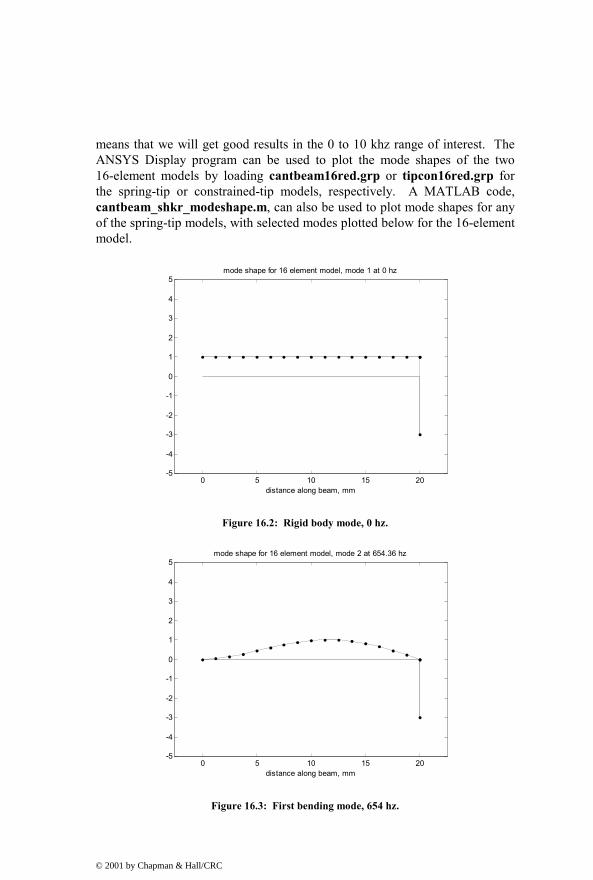
means that we will get good results in the 0 to 10 khz range of interest. The ANSYS Display program can be used to plot the mode shapes of the two 16-element models by loading cantbeam16red.grp or tipcon16red.grp for the spring-tip or constrained-tip models, respectively. A MATLAB code, cantbeam_shkr_modeshape.m, can also be used to plot mode shapes for any of the spring-tip models, with selected modes plotted below for the 16-element model.

0 5 10 15 20-5

-4

-3

-2

-1

0

1

2

3

4

5mode shape for 16 element model, mode 1 at 0 hz

distance along beam, mm

Figure 16.2: Rigid body mode, 0 hz.

0 5 10 15 20-5

-4

-3

-2

-1

0

1

2

3

4

5mode shape for 16 element model, mode 2 at 654.36 hz


Figure 16.3: First bending mode, 654 hz.


0 5 10 15 20-5

-4

-3

-2

-1

0

1

2

3

4

5mode shape for 16 element model, mode 3 at 2120.1 hz


Figure 16.4: Second bending mode, 2120 hz.

0 5 10 15 20-5

-4

-3

-2

-1

0

1

2

3

4

5mode shape for 16 element model, mode 10 at 32552 hz


Figure 16.5: Beam tip / Spring mode at 32552 hz.

Note the deflection at the tip involving the spring for mode 10 for the 16-element model. Since we are interested in using the spring deflections to measure force exerted at the beam tip constraint, we will find that including the 10th mode is important because of its large dc gain value.


16.4 MATLAB State Space Model from ANSYS Eigenvalue Run – cantbeam_ss_shkr_modred.m

The MATLAB code used in this chapter is very similar to the code in Chapter 15. As such, some of the following descriptions will refer to the previous chapter.

The results shown and discussed in this chapter will be for the 16-element beam model; however, ANSYS data is available for 2-, 4-, 8-, 10-, 12-, 16-, 32- and 64-beam elements.

16.4.1 Input

This Section is similar to that in Section 15.6.1, with the same options available for choosing the number of elements to be analyzed. Eigenvalue/eigenvector results for all the models are available in the respective MATLAB .mat files and are called based on which menu item is picked.

% cantbeam_ss_shkr_modred.m clear all; hold off; clf; % load the .mat file cantbeamXXred, containing evr - the modal matrix, freqvec - % the frequency vector and node_numbers - the vector of node numbers for the modal % matrix model = menu('choose which finite element model to use ... ', .... '2 beam elements', ... '4 beam elements', ... '6 beam elements', ... '8 beam elements', ... '10 beam elements', ... '12 beam elements', ... '16 beam elements', ... '32 beam elements', ... '64 beam elements'); if model == 1 load cantbeam2red_shkr; elseif model == 2 load cantbeam4red_shkr; elseif model == 3 load cantbeam6red_shkr; elseif model == 4


load cantbeam8red_shkr; elseif model == 5 load cantbeam10red_shkr; elseif model == 6 load cantbeam12red_shkr; elseif model == 7 load cantbeam16red_shkr; elseif model == 8 load cantbeam32red_shkr; elseif model == 9 load cantbeam64red_shkr; end

16.4.2 Shaker, Spring, Gram Force Definitions

The value of the beam tip spring stiffness is the same values as in the ANSYS code and is used to calculate the force between the beam tip and the shaker. The shaker mass value is the same value as in the ANSYS code and is used to define the force required in the MATLAB model to impart a desired acceleration level to the shaker. The force conversion from mN to gram force is defined as 1/9.807.

kspring = 1000000; % mN/mm from ANSYS run shaker_mass = 0.050; % kg from ANSYS run mn2gm_conversion = 0.101968; % conversion factor from mn to gram-f, 1/9.807

16.4.3 Defining Degrees of Freedom and Number of Modes

This section of code is identical to that of Section 15.6.2.

% define the number of degrees of freedom and number of modes from size of % modal matrix [numdof,num_modes_total] = size(evr); % define rows for shaker and tip nodes shaker_node_row = 1; tip_node_row = numdof; xn = evr;


16.4.4 Frequency Range, Sorting Modes by dc Gain and Plotting, Selecting Modes Used

As in Section 15.6.3, the next step in creating the model is to sort modes of vibration so that only the most important modes are kept. Repeating from Chapter 15 to obtain the frequency response at dc:

m

j nji nki2

i 1k i

z z zF =

=ω∑ , (16.1)

where the dc gain of for the ith mode is given by the expression:

ith mode dc gain: j nji nki2

k i

z z zF

= ω

(16.2)

The difference between the code below and the code in Section 15.6.3 is that we have a rigid body, 0 hz, mode in this model and the previous cantilever did not. The problem is in dividing (16.1) by 2 2

i 1 0ω = ω = , which would give a dc gain of infinity for the rigid body mode. In order to get around this, we do not use zero for the rigid body frequency but instead use the frequency response lower bound frequency for calculating a “low frequency” gain. In this model the lower bound frequency is 100 hz. Another method of ranking would be to rank only the non rigid body modes, recognizing that the rigid body mode is always included.

Once again, dc gain will be used to rank the relative importance of modes. The dc gain calculation for each mode, “dc_value,” is broken into two parts. The first part calculates the gain of the rigid body mode at the “freqlo” frequency while the second part calculates the dc gain of all the non rigid body modes.

The bulk of this section is similar to Section 15.6.3.

% calculate the dc amplitude of the displacement of each mode by % multiplying the forcing function row of the eigenvector by the output row omega2 = (2*pi*freqvec)'.^2; % convert to radians and square % define frequency range for frequency response freqlo = 100; freqhi = 100000;


flo=log10(freqlo) ; fhi=log10(freqhi) ; f=logspace(flo,fhi,200) ; frad=f*2*pi ; dc_gain = abs([xn(shaker_node_row,1)*xn(tip_node_row,1)/frad(1) ... (xn(shaker_node_row,2:num_modes_total) ... .*xn(tip_node_row,2:num_modes_total))./omega2(2:num_modes_total)]); [dc_gain_sort,index_sort] = sort(dc_gain); dc_gain_sort = fliplr(dc_gain_sort); index_sort = fliplr(index_sort) dc_gain_nosort = dc_gain;

index_orig = 1:num_modes_total; semilogy(index_orig,freqvec,'k-'); title('frequency versus mode number') xlabel('mode number') ylabel('frequency, hz') grid disp('execution paused to display figure, "enter" to continue'); pause semilogy(index_orig,dc_gain_nosort,'k-') title('dc value of each mode contribution versus mode number') xlabel('mode number') ylabel('dc value') grid disp('execution paused to display figure, "enter" to continue'); pause loglog([freqlo; freqvec(2:num_modes_total)],dc_gain_nosort,'k-') title('dc value of each mode contribution versus frequency') xlabel('frequency, hz') ylabel('dc value') grid disp('execution paused to display figure, "enter" to continue'); pause semilogy(index_orig,dc_gain_sort,'k-') title('sorted dc value of each mode versus number of modes included') xlabel('modes included') ylabel('sorted dc value') grid disp('execution paused to display figure, "enter" to continue'); pause num_modes_used = input(['enter how many modes to include, …

',num2str(num_modes_total),' default, max ... ']);

if (isempty(num_modes_used)) num_modes_used = num_modes_total; end


2 4 6 8 10 12 14 16 18102

103

104

105

106frequency versus mode number

mode number

frequ

ency

, hz

Figure 16.6: Resonant frequency versus mode number for 16-element model.

Figure 16.6 shows the resonant frequency versus mode number for the 16-element model, Reduced method of eigenvalue extraction, showing that modes six and higher have frequencies greater than the 10 khz frequency range of interest for this model. This would lead one to think that only the first six or eight modes would be required to define the force in the 0 to 10 khz frequency range, which is not the case as we shall see.

0 2 4 6 8 10 12 14 16 1810-14

10-12

10-10

10-8

10-6

10-4

10-2

100dc value of each mode contribution versus mode number

mode number

dc v

alue

Figure 16.7: Low frequency and dc gains versus mode number.


Figure 16.7 shows the low frequency gain for the rigid body mode, mode 1, and the dc gains for all other modes, versus mode number. Note that the second most important mode (the second highest dc gain) is mode 10, and that it is even more important than the first bending mode of the cantilever.

102 103 104 105 10610-14

10-12

10-10

10-8

10-6

10-4

10-2

100dc value of each mode contribution versus frequency

frequency, hz

dc v

alue

Figure 16.8: Low frequency and dc gain versus frequency.

Figure 16.8 shows the same data plotted against frequency instead of mode number. The tip mass / tip spring mode at 32552 hz is the mode with the high gain.

0 2 4 6 8 10 12 14 16 1810-14

10-12

10-10

10-8

10-6

10-4

10-2

100sorted dc value of each mode versus number of modes included

modes included

sorte

d dc

val

ue

Figure 16.9: Sorted low frequency and dc gains versus number of modes.


In Figure 16.9 we can see the sorted values for the low frequency and dc gains, from largest to smallest. The list of sorted mode numbers is given in the table below. Once again, the 10th mode is the second most significant after the rigid body mode.

index_sort = 1 10 2 4 9 8 6 11 3 12 5 13 14 7 15 16 17

Table 16.2: Sorted low frequency and dc gain indices.

16.4.5 Damping, Defining Reduced Frequencies and Modal Matrices

This section is exactly like that in Section 15.6.4.

zeta = input('enter value for damping, .02 is 2% of critical (default) ... ');

if (isempty(zeta)) zeta = .02;

end % all modes included model, use original order xnnew = xn(:,(1:num_modes_total)); freqnew = freqvec((1:num_modes_total)); % reduced, no sorting, just use the first num_modes_used modes in xnnew_nosort xnnew_nosort = xn(:,1:num_modes_used); freqnew_nosort = freqvec(1:num_modes_used); % reduced, sorting, use the first num_modes_used sorted modes in xnnew_sort xnnew_sort = xn(:,index_sort(1:num_modes_used)); freqnew_sort = freqvec(index_sort(1:num_modes_used));

16.4.6 Setting Up System Matrix “a”

This section is exactly like that in Section 15.6.5.

% define variables for all modes included system matrix, a

w = freqnew*2*pi; % frequencies in rad/sec w2 = w.^2;

zw = 2*zeta*w;


% define variables for reduced, nosorted system matrix, a_nosort

w_nosort = freqnew_nosort*2*pi; % frequencies in rad/sec w2_nosort = w_nosort.^2;

zw_nosort = 2*zeta*w_nosort; % define variables for reduced, sorted system matrix, a_sort

w_sort = freqnew_sort*2*pi; % frequencies in rad/sec w2_sort = w_sort.^2;

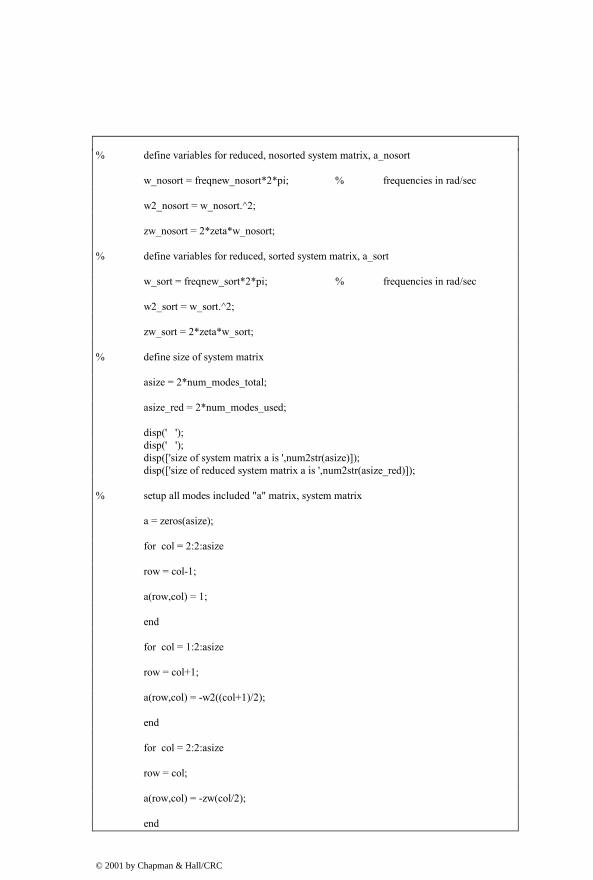
zw_sort = 2*zeta*w_sort; % define size of system matrix asize = 2*num_modes_total; asize_red = 2*num_modes_used; disp(' '); disp(' '); disp(['size of system matrix a is ',num2str(asize)]); disp(['size of reduced system matrix a is ',num2str(asize_red)]); % setup all modes included "a" matrix, system matrix a = zeros(asize); for col = 2:2:asize row = col-1; a(row,col) = 1; end for col = 1:2:asize row = col+1; a(row,col) = -w2((col+1)/2); end for col = 2:2:asize row = col; a(row,col) = -zw(col/2); end


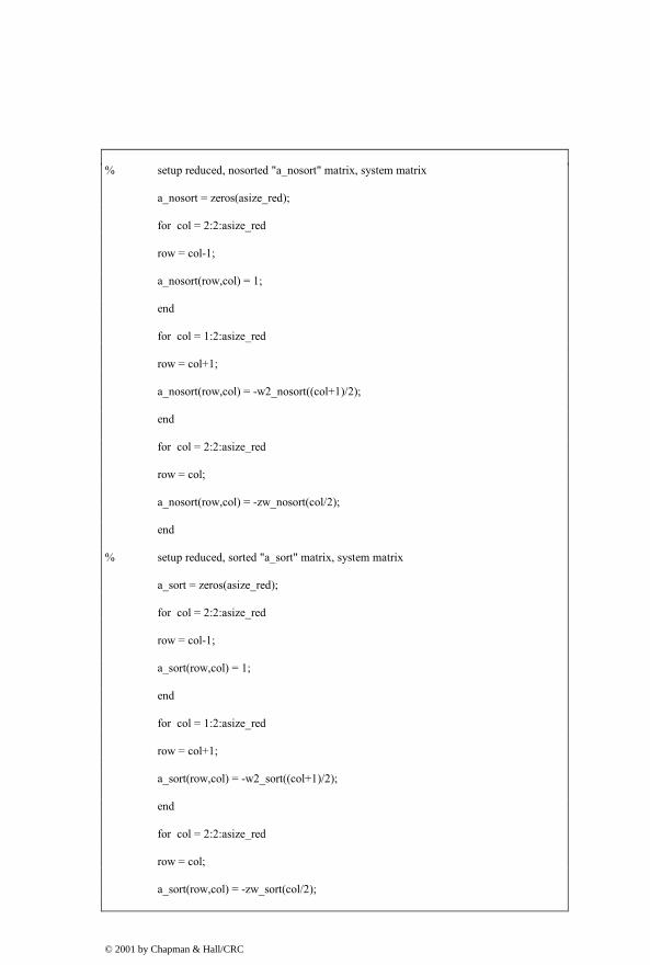
% setup reduced, nosorted "a_nosort" matrix, system matrix a_nosort = zeros(asize_red); for col = 2:2:asize_red row = col-1; a_nosort(row,col) = 1; end for col = 1:2:asize_red row = col+1; a_nosort(row,col) = -w2_nosort((col+1)/2); end for col = 2:2:asize_red row = col; a_nosort(row,col) = -zw_nosort(col/2); end % setup reduced, sorted "a_sort" matrix, system matrix a_sort = zeros(asize_red); for col = 2:2:asize_red row = col-1; a_sort(row,col) = 1; end for col = 1:2:asize_red row = col+1; a_sort(row,col) = -w2_sort((col+1)/2); end for col = 2:2:asize_red row = col; a_sort(row,col) = -zw_sort(col/2);


end

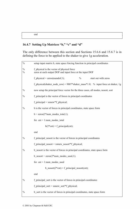
16.4.7 Setting Up Matrices “b,” “c” and “d”

The only difference between this section and Sections 15.6.6 and 15.6.7 is in defining the force to be applied to the shaker to give 1g acceleration.

% setup input matrix b, state space forcing function in principal coordinates % f_physical is the vector of physical force % zeros at each output DOF and input force at the input DOF f_physical = zeros(numdof,1); % start out with zeros f_physical(shaker_node_row) = 9807*shaker_mass*1.0; % input force at shaker, 1g % now setup the principal force vector for the three cases, all modes, nosort, sort % f_principal is the vector of forces in principal coordinates f_principal = xnnew'*f_physical; % b is the vector of forces in principal coordinates, state space form b = zeros(2*num_modes_total,1); for cnt = 1:num_modes_total b(2*cnt) = f_principal(cnt); end % f_principal_nosort is the vector of forces in principal coordinates f_principal_nosort = xnnew_nosort'*f_physical; % b_nosort is the vector of forces in principal coordinates, state space form b_nosort = zeros(2*num_modes_used,1); for cnt = 1:num_modes_used b_nosort(2*cnt) = f_principal_nosort(cnt); end % f_principal_sort is the vector of forces in principal coordinates f_principal_sort = xnnew_sort'*f_physical; % b_sort is the vector of forces in principal coordinates, state space form


b_sort = zeros(2*num_modes_used,1); for cnt = 1:num_modes_used b_sort(2*cnt) = f_principal_sort(cnt); end % setup cdisp and cvel, padded xn matrices to give the displacement and velocity % vectors in physical coordinates % cdisp and cvel each have numdof rows and alternating columns consisting of columns % of xnnew and zeros to give total columns equal to the number of states % all modes included cdisp and cvel for col = 1:2:2*length(freqnew) for row = 1:numdof cdisp(row,col) = xnnew(row,ceil(col/2)); cvel(row,col) = 0; end end for col = 2:2:2*length(freqnew) for row = 1:numdof cdisp(row,col) = 0; cvel(row,col) = xnnew(row,col/2); end end % reduced, nosorted cdisp and cvel for col = 1:2:2*length(freqnew_nosort) for row = 1:numdof cdisp_nosort(row,col) = xnnew_nosort(row,ceil(col/2)); cvel_nosort(row,col) = 0; end end for col = 2:2:2*length(freqnew_nosort)


for row = 1:numdof cdisp_nosort(row,col) = 0; cvel_nosort(row,col) = xnnew_nosort(row,col/2); end end % reduced, sorted cdisp and cvel for col = 1:2:2*length(freqnew_sort) for row = 1:numdof cdisp_sort(row,col) = xnnew_sort(row,ceil(col/2)); cvel_sort(row,col) = 0; end end for col = 2:2:2*length(freqnew_sort) for row = 1:numdof cdisp_sort(row,col) = 0; cvel_sort(row,col) = xnnew_sort(row,col/2); end end % define output d = [0]; %

16.4.8 “ss” Setup, Bode Calculations

This section differs from that of Section 15.6.8 in that the frequency range definition that exists in 15.6.8 was moved earlier in this code to allow the use of “freqlo” to calculate the low frequency gain of the rigid body mode. Also, the “ss” model below for “sysforce” directly calculates the force in the spring by subtracting the displacement of the shaker from that beam tip and multiplying the difference by the spring stiffness and the mN to gram force conversion. The output then indicates the variation of force between the beam tip and the shaker, or for the disk drive the variation in force which is


preloading the recording head to the disk. If the variation in force exceeds the preload force, the head will tend to unload.

% define tip force state space system with the "ss" command sysforce = ss(a,b,mn2gm_conversion*kspring*(cdisp(tip_node_row,:)- …

cdisp(shaker_node_row,:)),d); % define reduced system using nosort modes sysforce_nosort = ss(a_nosort,b_nosort,mn2gm_conversion*kspring* …

(cdisp_nosort(tip_node_row,:)-cdisp_nosort(shaker_node_row,:)),d); % define reduced system using sorted modes sysforce_sort = ss(a_sort,b_sort,mn2gm_conversion*kspring* …

(cdisp_sort(tip_node_row,:)-cdisp_sort(shaker_node_row,:)),d); % use "bode" command to generate magnitude/phase vectors [magforce,phsforce] = bode(sysforce,frad); [magforce_nosort,phsforce_nosort] = bode(sysforce_nosort,frad); [magforce_sort,phsforce_sort] = bode(sysforce_sort,frad);

16.4.9 Full Model – Plotting Frequency Response, Shock Response

The code in this section is similar to that in Section 15.6.9, where the overall frequency response and its individual mode contributions are plotted. The “lsim” command is used to calculate the response to a half-sine shock pulse.

% start plotting if num_modes_used == num_modes_total % plot all modes included response loglog(f,magforce(1,:),'k.-') title(['cantilever tip force for mid-length force, all ',num2str(num_modes_used), …

' modes included']) xlabel('Frequency, hz') ylabel('Force, gm') grid on disp('execution paused to display figure, "enter" to continue'); pause hold on max_modes_plot = num_modes_used; for pcnt = 1:max_modes_plot


index = 2*pcnt; amode = a_nosort(index-1:index,index-1:index); bmode = b_nosort(index-1:index); cmode_shaker = cdisp_nosort(1,index-1:index); cmode_tip = cdisp_nosort(numdof,index-1:index); dmode = [0]; sysforce_mode = ss(amode,bmode,mn2gm_conversion*kspring* …

(cmode_tip - cmode_shaker),dmode); [magforce_mode,phsforce_mode]=bode(sysforce_mode,frad) ; loglog(f,magforce_mode(1,:),'k-') end disp('execution paused to display figure, "enter" to continue'); pause hold off % now use lsim to calculate force due to a 0.002 sec half-sine 100g shock pulse ttotal = 0.03; shock_amplitude = 100; pulse_width = input('enter half-sine shock pulse width, sec, default is 0.002 ... '); if isempty(pulse_width) pulse_width = 0.002; end t = linspace(0,ttotal,1000); dt = t(2) - t(1); for cnt = 1:length(t) if t(cnt) < pulse_width u(cnt) = shock_amplitude*sin(2*pi*(1/(2*pulse_width))*t(cnt)); else u(cnt) = 0; end end


plot(t,u,'k-') title('acceleration of shaker mass') xlabel('time, sec') ylabel('acceleration, g') grid on disp('execution paused to display figure, "enter" to continue'); pause [force,ts] = lsim(sysforce,u,t); plot(ts,force,'k-') title(['cantilever tip force for ',num2str(shock_amplitude),'g, ',num2str(pulse_width) ... ,' sec input, all ',num2str(num_modes_used),' modes included']) xlabel('time, sec') ylabel('Force, gm') grid on disp('execution paused to display figure, "enter" to continue'); pause peak_force = max(abs(force))

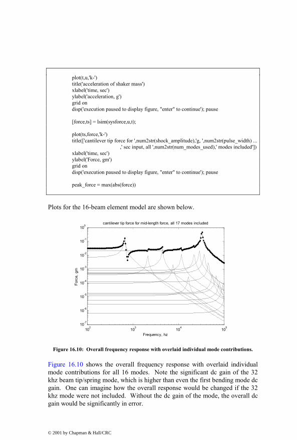
Plots for the 16-beam element model are shown below.

102 103 104 10510-7

10-6

10-5

10-4

10-3

10-2

10-1

100cantilever tip force for mid-length force, all 17 modes included

Frequency, hz

Forc

e, g

m

Figure 16.10: Overall frequency response with overlaid individual mode contributions.

Figure 16.10 shows the overall frequency response with overlaid individual mode contributions for all 16 modes. Note the significant dc gain of the 32 khz beam tip/spring mode, which is higher than even the first bending mode dc gain. One can imagine how the overall response would be changed if the 32 khz mode were not included. Without the dc gain of the mode, the overall dc gain would be significantly in error.


0 0.005 0.01 0.015 0.02 0.025 0.030

10

20

30

40

50

60

70

80

90

100acceleration of shaker mass

time, sec

acce

lera

tion,

g

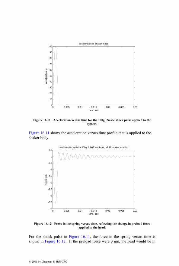
Figure 16.11: Acceleration versus time for the 100g, 2msec shock pulse applied to the system.

Figure 16.11 shows the acceleration versus time profile that is applied to the shaker body.

0 0.005 0.01 0.015 0.02 0.025 0.03-4

-3.5

-3

-2.5

-2

-1.5

-1

-0.5

0

0.5cantilever tip force for 100g, 0.002 sec input, all 17 modes included

time, sec

Forc

e, g

m

Figure 16.12: Force in the spring versus time, reflecting the change in preload force applied to the head.

For the shock pulse in Figure 16.11, the force in the spring versus time is shown in Figure 16.12. If the preload force were 3 gm, the head would be in


danger of unloading from the disk since the peak variation in preload force is 3.6 gm.

16.4.10 Reduced Models – Plotting Frequency Response, Shock Response

This section is similar to Section 15.6.10, setting up frequency response and half-sine shock response for sorted and unsorted modes.

else % unsorted modal truncation loglog(f,magforce(1,:),'k-',f,magforce_nosort(1,:),'k.-') title(['unsorted modal truncation: cantilever tip force for mid-length force, …

first ',num2str(num_modes_used),' modes included']) legend('all modes','unsorted partial modes',3) dcgain_error_percent_nosort = 100*(magforce_nosort(1) - magforce(1))/magforce(1) xlabel('Frequency, hz') ylabel('Force, gm') grid on disp('execution paused to display figure, "enter" to continue'); pause hold on max_modes_plot = num_modes_used; for pcnt = 1:max_modes_plot index = 2*pcnt; amode = a_nosort(index-1:index,index-1:index); bmode = b_nosort(index-1:index); cmode_shaker = cdisp_nosort(1,index-1:index); cmode_tip = cdisp_nosort(numdof,index-1:index); dmode = [0]; sysforce_mode = ss(amode,bmode,mn2gm_conversion*kspring* …

(cmode_tip - cmode_shaker),dmode); [magforce_mode,phsforce_mode]=bode(sysforce_mode,frad) ; loglog(f,magforce_mode(1,:),'k-') end disp('execution paused to display figure, "enter" to continue'); pause


hold off % sorted modal truncation loglog(f,magforce(1,:),'k-',f,magforce_sort(1,:),'k.-') title(['sorted modal truncation: cantilever tip force for mid-length force, …

first ',num2str(num_modes_used),' modes included']) legend('all modes','sorted partial modes',3) dcgain_error_percent_sort = 100*(magforce_sort(1) - magforce(1))/magforce(1) xlabel('Frequency, hz') ylabel('Force, gm') grid on disp('execution paused to display figure, "enter" to continue'); pause hold on % now plot the overlay of the tip force magnitude with each mode contribution max_modes_plot = num_modes_used; for pcnt = 1:max_modes_plot index = 2*pcnt; amode = a_nosort(index-1:index,index-1:index); bmode = b_nosort(index-1:index); cmode_shaker = cdisp_nosort(1,index-1:index); cmode_tip = cdisp_nosort(numdof,index-1:index); dmode = [0]; sysforce_mode = ss(amode,bmode,mn2gm_conversion*kspring* …

(cmode_tip - cmode_shaker),dmode); [magforce_mode,phsforce_mode]=bode(sysforce_mode,frad) ; loglog(f,magforce_mode(1,:),'k-') end disp('execution paused to display figure, "enter" to continue'); pause hold off % now use lsim to calculate force due to a 0.002 sec half-sine 100g shock pulse ttotal = 0.03;


shock_amplitude = 100; pulse_width = input('enter half-sine shock pulse width, sec, default is 0.002 ... '); if isempty(pulse_width) pulse_width = 0.002; end t = linspace(0,ttotal,1000); dt = t(2) - t(1); for cnt = 1:length(t) if t(cnt) < pulse_width u(cnt) = shock_amplitude*sin(2*pi*(1/(2*pulse_width))*t(cnt)); else u(cnt) = 0; end end plot(t,u,'k-') title('acceleration of shaker mass') xlabel('time, sec') ylabel('acceleration, g') grid on disp('execution paused to display figure, "enter" to continue'); pause [force,ts] = lsim(sysforce,u,t); [force_nosort,ts_nosort] = lsim(sysforce_nosort,u,t); [force_sort,ts_sort] = lsim(sysforce_sort,u,t); plot(ts,force,'k-',ts_nosort,force_nosort,'k+:',ts_sort,force_sort,'k.-') title(['cantilever tip force for ',num2str(shock_amplitude),'g, ',num2str(pulse_width) ... ,' sec input, ',num2str(num_modes_used),' modes included']) legend('all modes','unsorted partial modes','sorted partial modes',4) xlabel('time, sec') ylabel('Force, gm') grid on disp('execution paused to display figure, "enter" to continue'); pause max_force = max(abs(force)); max_force_nosort = max(abs(force_nosort)); max_force_sort = max(abs(force_sort)); error_nosort_percent = 100*(max_force_nosort - max_force)/max_force error_sort_percent = 100*(max_force_sort - max_force)/max_force


16.4.11 Reduced Models – Plotted Results, Four Modes Used

Note that in all the frequency response plots that follow, the title will indicate that “four” modes are included, the four being the rigid body mode at 0 hz and the first three either sorted or unsorted resonances. Because we are subtracting the displacement of the tip from the displacement of the shaker to find the force in the spring, the rigid body mode is effectively subtracted out, allowing us to see the detailed motion of the beam/mass relative to the shaker. This is why the rigid body mode does not show up as one of the four individual modes used.

102 103 104 10510-7

10-6

10-5

10-4

10-3

10-2

10-1

100unsorted modal truncation: cantilever tip force for mid-length force, first 4 modes included

Frequency, hz

Forc

e, g

m

all modes unsorted partial modes

Figure 16.13: Overall plus individual mode contributions for the four unsorted mode model.

In Figure 16.13 the first four unsorted modes are used, so the 32 khz beam tip mode is not included and the overall response is poor. Both the dc gain and high frequency behavior are badly in error. The dc gain error is 75%.


102 103 104 10510-7

10-6

10-5

10-4

10-3

10-2

10-1

100sorted modal truncation: cantilever tip force for mid-length force, first 4 modes included

Frequency, hz

Forc

e, g

m

all modes sorted partial modes

Figure 16.14: Overall plus individual mode contributions for the four sorted mode model.

In Figure 16.14 the 32 khz beam tip mode is one of the included modes. Both the overall dc gain and high frequency behavior are quite good matches with the “all modes included” model with only four modes included. The dc gain error is –6.2%.

0 0.005 0.01 0.015 0.02 0.025 0.03-4

-3.5

-3

-2.5

-2

-1.5

-1

-0.5

0

0.5cantilever tip force for 100g, 0.002 sec input, 4 modes included

time, sec

Forc

e, g

m

all modes unsorted partial modessorted partial modes

Figure 16.15: Half-sine shock pulse response for full, reduced unsorted and reduced sorted models.


Figure 16.15 shows the how the dc gain error in the frequency domain for the unsorted model shows up as a significant error in peak response in the time domain, 67%. The error in the sorted peak response is only 5.6%.

16.4.12 Modred – Setting up, “mdc” and “del” Reduction, Bode Calculations

In this section the user is prompted for whether to use the sorted or original mode order, then the corresponding system matrices are defined. The “modred” command is used with both the “mdc” and “del” options to define two reduced systems. The “bode” command is used to calculate frequency responses.

% use modred to reduce, select whether to use sorted or unsorted modes for the reduction modred_sort = input('modred: enter "1" to use sorted modes for reduced runs, …

"enter" to use unsorted ... '); if isempty(modred_sort) modred_sort = 0 end if modred_sort == 1 % use sorted mode order xnnew = xn(:,index_sort(1:num_modes_total)); freqnew = freqvec(index_sort(1:num_modes_total)); else % use original mode order xnnew = xn(:,(1:num_modes_total)); freqnew = freqvec((1:num_modes_total)); end % define variables for all modes included system matrix, a

w = freqnew*2*pi; % frequencies in rad/sec w2 = w.^2;

zw = 2*zeta*w; % setup all modes included "a" matrix, system matrix a = zeros(asize); for col = 2:2:asize row = col-1;


a(row,col) = 1; end for col = 1:2:asize row = col+1; a(row,col) = -w2((col+1)/2); end for col = 2:2:asize row = col; a(row,col) = -zw(col/2); end % setup input matrix b, state space forcing function in principal coordinates % f_physical is the vector of physical force % zeros at each output DOF and input force at the input DOF f_physical = zeros(numdof,1); % start out with zeros f_physical(shaker_node_row) = 9807*shaker_mass*1.0; % input force at shaker, 1g % now setup the principal force vector for the three cases, all modes, nosort, sort % f_principal is the vector of forces in principal coordinates f_principal = xnnew'*f_physical; % b is the vector of forces in principal coordinates, state space form b = zeros(2*num_modes_total,1); for cnt = 1:num_modes_total b(2*cnt) = f_principal(cnt); end % setup cdisp and cvel, padded xn matrices to give the displacement and velocity % vectors in physical coordinates % cdisp and cvel each have numdof rows and alternating columns consisting of columns % of xnnew and zeros to give total columns equal to the number of states % all modes included cdisp and cvel for col = 1:2:2*length(freqnew) for row = 1:numdof


cdisp(row,col) = xnnew(row,ceil(col/2)); cvel(row,col) = 0; end end for col = 2:2:2*length(freqnew) for row = 1:numdof cdisp(row,col) = 0; cvel(row,col) = xnnew(row,col/2); end end % define output d = [0]; % % define state space system for reduction, ordered defined by modred_sort sysforce_red = ss(a,b,mn2gm_conversion*kspring*(cdisp(tip_node_row,:)- …

cdisp(shaker_node_row,:)),d); % define reduced matrices using matched dc gain method "mdc" states_elim = (2*num_modes_used+1):2*num_modes_total; sysforce_mdc = modred(sysforce_red,states_elim,'mdc'); [aforce_mdc,bforce_mdc,cforce_mdc,dforce_mdc] = ssdata(sysforce_mdc); % define reduced matrices by eliminating high frequency states, 'del' sysforce_elim = modred(sysforce_red,states_elim,'del'); [aforce_elim,bforce_elim,cforce_elim,dforce_elim] = ssdata(sysforce_elim); % use "bode" command to generate magnitude/phase vectors for reduced systems [magforce_mdc,phsforce_mdc]=bode(sysforce_mdc,frad) ; [magforce_elim,phsforce_elim]=bode(sysforce_elim,frad) ; % convert magnitude to db magforce_mdcdb = 20*log10(magforce_mdc); magforce_elimdb = 20*log10(magforce_elim);


16.4.13 Reduced Modred Models – Plotting Commands

Both the “del” and “mdc” reduced systems are plotted and compared with the original, non-reduced system. The individual mode contributions to the two reduced responses are also plotted.

% start plotting % modred using 'elim' loglog(f,magforce(1,:),'k-',f,magforce_elim(1,:),'k.-') if modred_sort == 1 title(['reduced elimination: cantilever tip force for mid-length force, …

first ',num2str(num_modes_used),' sorted modes included']) dcgain_error_percent_elim_sort = 100*(magforce_elim(1) …

- magforce(1))/magforce(1) else title(['reduced elimination: cantilever tip force for mid-length force, …

first ',num2str(num_modes_used),' unsorted modes included']) dcgain_error_percent_elim_nosort = 100*(magforce_elim(1) …

- magforce(1))/magforce(1) end legend('all modes','reduced elimination',3) xlabel('Frequency, hz') ylabel('Force, gm') grid on disp('execution paused to display figure, "enter" to continue'); pause hold on max_modes_plot = num_modes_used; for pcnt = 1:max_modes_plot index = 2*pcnt; amode = aforce_elim(index-1:index,index-1:index); bmode = bforce_elim(index-1:index); cmode = cforce_elim(1,index-1:index); dmode = [0]; sysforce_mode = ss(amode,bmode,cmode,dmode); [magforce_mode,phsforce_mode]=bode(sysforce_mode,frad) ; loglog(f,magforce_mode(1,:),'k-')


end disp('execution paused to display figure, "enter" to continue'); pause hold off % modred using 'mdc' loglog(f,magforce(1,:),'k-',f,magforce_mdc(1,:),'k.-') if modred_sort == 1 title(['reduced matched dc gain: cantilever tip force for mid-length …

force, first ',num2str(num_modes_used),' sorted modes included']) dcgain_error_percent_mdc_sort = 100*(magforce_mdc(1) …

- magforce(1))/magforce(1) else title(['reduced matched dc gain: cantilever tip force for mid-length …

f orce, first ',num2str(num_modes_used),' unsorted modes included']) dcgain_error_percent_mdc_nosort = 100*(magforce_mdc(1) …

- magforce(1))/magforce(1) end legend('all modes','reduced mdc',3) xlabel('Frequency, hz') ylabel('Force, gm') grid on disp('execution paused to display figure, "enter" to continue'); pause hold on max_modes_plot = num_modes_used; for pcnt = 1:max_modes_plot index = 2*pcnt; amode = aforce_mdc(index-1:index,index-1:index); bmode = bforce_mdc(index-1:index); cmode = cforce_mdc(1,index-1:index); dmode = [0]; sysforce_mode = ss(amode,bmode,cmode,dmode); [magforce_mode,phsforce_mode]=bode(sysforce_mode,frad) ; loglog(f,magforce_mode(1,:),'k-') end


disp('execution paused to display figure, "enter" to continue'); pause hold off % now use lsim to calculate force due to a 0.002 sec half-sine 100g shock pulse [force_mdc,ts_mdc] = lsim(sysforce_mdc,u,t); [force_elim,ts_elim] = lsim(sysforce_elim,u,t); plot(ts,force,'k-',ts_mdc,force_mdc,'k.-',ts_elim,force_elim,'k+-') if modred_sort == 1 title(['modred cantilever tip force for ',num2str(shock_amplitude),'g, …

',num2str(pulse_width) ,' sec input, ',num2str(num_modes_used), … ' sorted modes included'])

else title(['modred cantilever tip force for ',num2str(shock_amplitude),'g, …

',num2str(pulse_width) ,' sec input, ',num2str(num_modes_used), … ' unsorted modes included'])

end legend('all modes','reduced - mdc','reduced - elim',4) xlabel('time, sec') ylabel('Force, gm') grid on disp('execution paused to display figure, "enter" to continue'); pause max_force_mdc = max(abs(force_mdc)); max_force_elim = max(abs(force_elim)); peak_error_mdc_percent = 100*(max_force_mdc - max_force)/max_force peak_error_elim_percent = 100*(max_force_elim - max_force)/max_force end

16.4.14 Plotting Unsorted Modred Reduced Results – Eliminating High Frequency Modes

This section looks at how well “modred” performs when unsorted modes are used. We will see that the “del” option using the first four unsorted modes does a poor job of matching the original response while the “mdc” option using the same four unsorted modes does a good job of matching the lower frequency range of the response while missing the tenth mode resonance. The overall transient response of the system is matched well by the “mdc” option while the “del” option has significant error.


102 103 104 10510-7

10-6

10-5

10-4

10-3

10-2

10-1

100reduced elimination: cantilever tip force for mid-length force, first 4 unsorted modes included

Frequency, hz

Forc

e, g

m

all modes reduced elimination

Figure 16.16: Overall frequency response with overload individual mode contributions for unsorted “del” modred option, with the 12 highest frequency modes eliminated.

Figure 16.16 displays the same response as the “unsorted” plot in Figure 16.13 because the “del” option in modred and our simple modal truncation method are equivalent. The dc gain is in error by 75%.

102 103 104 10510-7

10-6

10-5

10-4

10-3

10-2

10-1

100reduced matched dc gain: cantilever tip force for mid-length force, first 4 unsorted modes included

Frequency, hz

Forc

e, g

m

all modes reduced mdc

Figure 16.17: Overall frequency response with overlaid individual mode contributions for unsorted “mdc” modred option, with the 12 highest frequency modes reduced.


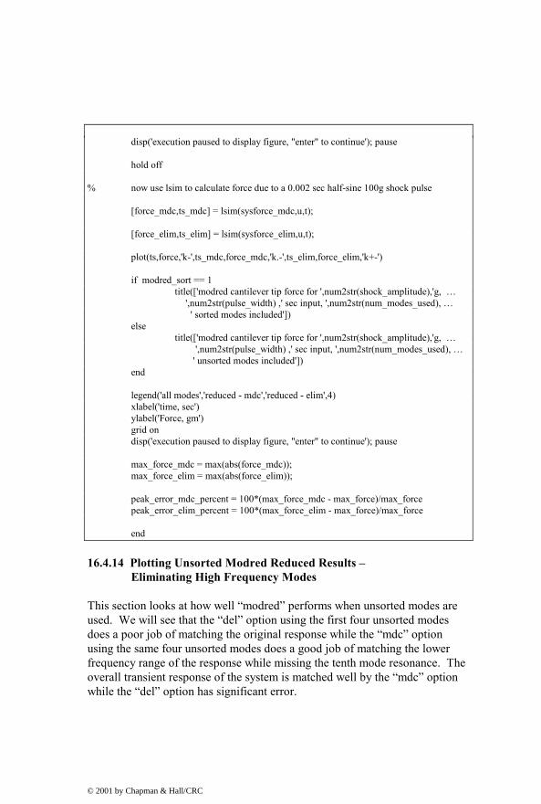
In Figure 16.17, the dc error is very small, 0.0008%. Even though the 32 khz mode is not included, the gain in the portion from 1 to 20 khz is close to the full model gain.

0 0.005 0.01 0.015 0.02 0.025 0.03-4

-3.5

-3

-2.5

-2

-1.5

-1

-0.5

0

0.5modred cantilever tip force for 100g, 0.002 sec input, 4 unsorted modes included

time, sec

Forc

e, g

m

all modes reduced - mdc reduced - elim

Figure 16.18: Half-sine shock pulse response for full, reduced unsorted “mdc” and reduced unsorted “del” models.

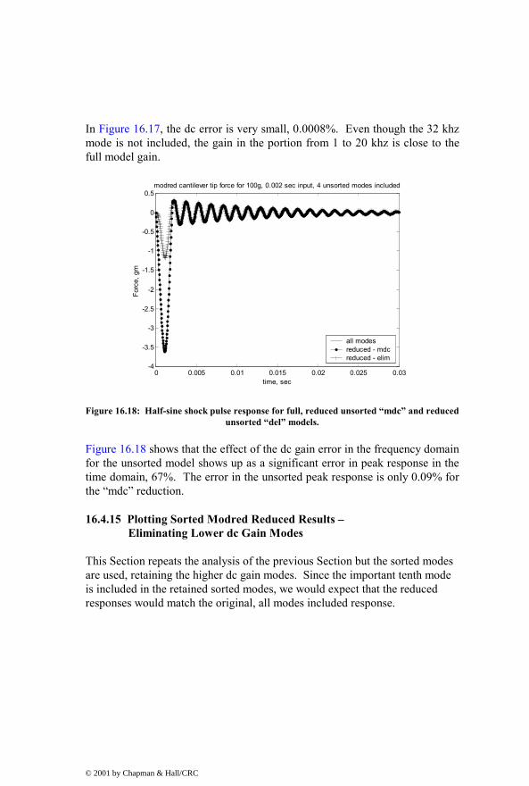
Figure 16.18 shows that the effect of the dc gain error in the frequency domain for the unsorted model shows up as a significant error in peak response in the time domain, 67%. The error in the unsorted peak response is only 0.09% for the “mdc” reduction.

16.4.15 Plotting Sorted Modred Reduced Results – Eliminating Lower dc Gain Modes

This Section repeats the analysis of the previous Section but the sorted modes are used, retaining the higher dc gain modes. Since the important tenth mode is included in the retained sorted modes, we would expect that the reduced responses would match the original, all modes included response.


102 103 104 10510-7

10-6

10-5

10-4

10-3

10-2

10-1

100reduced elimination: cantilever tip force for mid-length force, first 4 sorted modes included

Frequency, hz

Forc

e, g

m

all modes reduced elimination

Figure 16.19: Overall frequency response with overload individual mode contributions for sorted “del” modred option, with the 12 lowest dc gain modes eliminated.

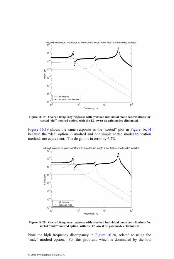
Figure 16.19 shows the same response as the “sorted” plot in Figure 16.14 because the “del” option in modred and our simple sorted modal truncation methods are equivalent. The dc gain is in error by 6.2%.

102 103 104 10510-7

10-6

10-5

10-4

10-3

10-2

10-1

100reduced matched dc gain: cantilever tip force for mid-length force, first 4 sorted modes included

Frequency, hz

Forc

e, g

m

all modes reduced mdc

Figure 16.20: Overall frequency response with overload individual mode contributions for sorted “mdc” modred option, with the 12 lowest dc gain modes eliminated.

Note the high frequency discrepancy in Figure 16.20, related to using the “mdc” modred option. For this problem, which is dominated by the low


frequency (<10khz) response and the dc gain of the 32 khz mode, the high frequency response is not important. The dc gain is in error by only 0.0025%.

0 0.005 0.01 0.015 0.02 0.025 0.03-4

-3.5

-3

-2.5

-2

-1.5

-1

-0.5

0

0.5modred cantilever tip force for 100g, 0.002 sec input, 4 sorted modes included

time, sec

Forc

e, g

m

all modes reduced - mdc reduced - elim

Figure 16.21: Half-sine shock pulse response for full, reduced unsorted and reduced sorted models.

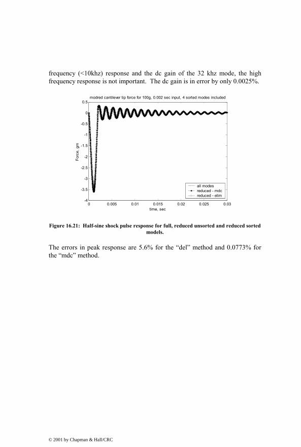
The errors in peak response are 5.6% for the “del” method and 0.0773% for the “mdc” method.


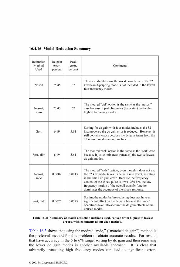
16.4.16 Model Reduction Summary

Reduction

Method Used

Dc gain error,

percent

Peak error,

percent

Comments

Nosort

75.45

67

This case should show the worst error because the 32 khz beam tip/spring mode is not included in the lowest four frequency modes.

Nosort, elim

75.45

67

The modred “del” option is the same as the “nosort” case because it just eliminates (truncates) the twelve highest frequency modes.

Sort

6.19

5.61

Sorting for dc gain with four modes includes the 32 khz mode, so the dc gain error is reduced. However, it still contains errors because the dc gain terms from the 12 unused modes are not included.

Sort, elim

6.19

5.61

The modred “del” option is the same as the “sort” case because it just eliminates (truncates) the twelve lowest dc gain modes.

Nosort, mdc

0.0007

0.0913

The modred “mdc” option, even though it does not use the 32 khz mode, takes its dc gain into effect, resulting in the small dc gain error. Because the frequency content of the shock pulse is low (~250 hz), the low frequency portion of the overall transfer function dominates the accuracy of the shock response.

Sort, mdc

0.0025

0.0773

Sorting the modes before reducing does not have a significant effect on the dc gain because the “mdc” operations take into account the dc gain effects of the unused modes.

Table 16.3: Summary of model reduction methods used, ranked from highest to lowest errors, with comments about each method.

Table 16.3 shows that using the modred “mdc,” (“matched dc gain”) method is the preferred method for this problem to obtain accurate results. For results that have accuracy in the 5 to 6% range, sorting by dc gain and then removing the lower dc gain modes is another available approach. It is clear that arbitrarily truncating high frequency modes can lead to significant errors


because a single, important mode is neglected. Another source of error would occur if the ANSYS model had not included enough elements (modes) to take into account the beam tip mode or if a selected range of eigenvalues had not included the mode.

In summary, every model reduction problem provides new challenges and needs to be analyzed before making a decision about which reduction method is most appropriate.

16.5 ANSYS Code cantbeam_ss_spring_shkr.inp Listing

The ANSYS code in this section is similar to the code cantbeam_ss.inp in Section 15.7 with the exception that a tip spring and “shaker” mass are added.

! cantbeam_ss_spring_shkr.inp, 0.075 thick x 2 wide x 20mm long steel cant with tip ! mass and spring on shaker, shaker mass at cantilever base and coupled to spring ground ! title automatically built based on number of elements and eigenvalue extraction method /prep7 filename = 'cantbeam_ss_spring_shkr' ! define number of elements to use num_elem = 10 ! define eigenvalue extraction method, 1 = reduced, 2 = block lanczos eigext = 2 *if,eigext,eq,1, then nummodes = num_elem+1 ! only 1 displacement dof available for each element *else nummodes = 2*(num_elem+1) ! both disp and rotation dof's available for each

! element *endif ! create the file name for storing data ! first section of filename aname = 'cantbeam' ! second section of filename, number of elements bname = num_elem ! third section of filename, depends on eigenvalue extraction method


*if,eigext,ne,2, then cname = 'red' ! reduced *else cname = 'bl' ! block Lanczos *endif ! input the title, use %xxx% to substitute parameter name or parametric expression aname_ti = 'cantbeam' /title,%aname_ti%, %bname%, %cname%, spring tip et,1,4 ! element type for beam et,2,14 ! element type for spring et,3,21 ! element type for mass ! steel ex,1,190e6 ! mN/mm^2 dens,1,7.83e-6 ! kg/mm^3 nuxy,1,0.293 ! real value to define beam characteristics r,1,0.15,0.05,0.00007031,0.075,0.2 ! beam properties: area, Izz, Iyy, TKz, TKy r,2,1000000 ! spring stiffness, mN/mm r,3,0.00002349,0.00002349,0.00002349 ! mass at tip, Kg r,4,0.050,0.050,0.050 ! shaker mass, Kg, approximately 1000 times mass ! define plotting characteristics /view,1,1,-1,1 ! iso view /angle,1,-60 ! iso view /pnum,mat,1 ! color by material /num,1 ! numbers off /type,1,0 ! hidden plot /pbc,all,1 ! show all boundary conditions csys,0 ! define global coordinate system ! nodes n,1,0,0,0 ! left-hand node n,num_elem+1,20,0,0 ! right-hand node fill,1,num_elem+1 ! interior nodes n,num_elem+2,20,0,-3 ! spring connection node nall nplo ! elements ! beam


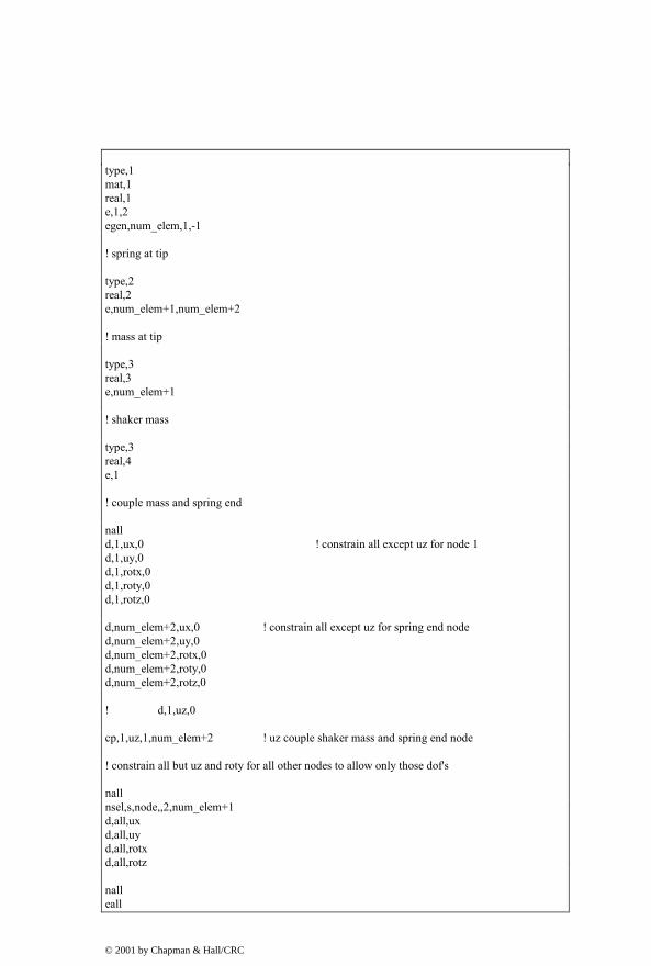
type,1 mat,1 real,1 e,1,2 egen,num_elem,1,-1 ! spring at tip type,2 real,2 e,num_elem+1,num_elem+2 ! mass at tip type,3 real,3 e,num_elem+1 ! shaker mass type,3 real,4 e,1 ! couple mass and spring end nall d,1,ux,0 ! constrain all except uz for node 1 d,1,uy,0 d,1,rotx,0 d,1,roty,0 d,1,rotz,0 d,num_elem+2,ux,0 ! constrain all except uz for spring end node d,num_elem+2,uy,0 d,num_elem+2,rotx,0 d,num_elem+2,roty,0 d,num_elem+2,rotz,0 ! d,1,uz,0 cp,1,uz,1,num_elem+2 ! uz couple shaker mass and spring end node ! constrain all but uz and roty for all other nodes to allow only those dof's nall nsel,s,node,,2,num_elem+1 d,all,ux d,all,uy d,all,rotx d,all,rotz nall eall


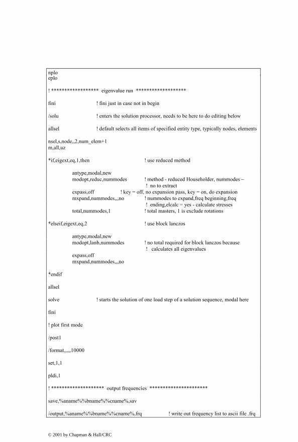
nplo eplo ! ****************** eigenvalue run ******************* fini ! fini just in case not in begin /solu ! enters the solution processor, needs to be here to do editing below allsel ! default selects all items of specified entity type, typically nodes, elements nsel,s,node,,2,num_elem+1 m,all,uz *if,eigext,eq,1,then ! use reduced method antype,modal,new modopt,reduc,nummodes ! method - reduced Householder, nummodes –

! no to extract expass,off ! key = off, no expansion pass, key = on, do expansion mxpand,nummodes,,,no ! nummodes to expand,freq beginning,freq

! ending,elcalc = yes - calculate stresses total,nummodes,1 ! total masters, 1 is exclude rotations *elseif,eigext,eq,2 ! use block lanczos antype,modal,new modopt,lanb,nummodes ! no total required for block lanczos because

! calculates all eigenvalues expass,off mxpand,nummodes,,,no *endif allsel solve ! starts the solution of one load step of a solution sequence, modal here fini ! plot first mode /post1 /format,,,,,10000 set,1,1 pldi,1 ! ******************** output frequencies ********************** save,%aname%%bname%%cname%,sav /output,%aname%%bname%%cname%,frq ! write out frequency list to ascii file .frq


set,list /output,term ! returns output to terminal ! ********************* output eigenvectors ******************* ! define nodes for output: forces applied or output displacements nsel,s,node,,1,num_elem+1 /output,%aname%%bname%%cname%,eig ! write out frequency list to ascii file .eig *do,i,1,nummodes set,,i /page,,,1000 prdisp *enddo /output,term ! ******************* plot modes ****************** ! pldi plots /show,%aname%%bname%%cname%,grp,0 ! save mode shape plots to file .grp allsel /view,1,,-1,, ! side view for plotting /angle,1,0 /auto *do,i,1,nummodes set,1,i pldi,1 *enddo /show,term


chapter 16: ground acceleration matlab model from ansys...

Documents