chapter 14fletcher/super/chap14.pdf334 14. two-way anova. 14.1.1 initial analysis. one way to view...
TRANSCRIPT


Chapter 14
Two-Way Anova
This chapter involves many model comparisons so, for simplicity within a given section, say 14.2,equation numbers such as (14.2.1) that redundantly specify the section number, are referred to in thetext without the section number, hence simply as (1). When referring to an equation number outsidethe current section, the full equation number is given.
14.1 Unbalanced two-way analysis of variance
Bailey (1953), Scheffe (1959), and Christensen (2011) examined data on infant female rats that weregiven to foster mothers for nursing. The variable of interest was the weight of the rat at 28 days.Weights were measured in grams. Rats are classified into four genotypes: A, F, I, and J. Specifically,rats from litters of each genotype were given to a foster mother of each genotype. The data arepresented in Table 14.1.
Table 14.1: Infant rats weight gain with foster mothers.
Genotype of Genotype of Foster MotherLitter A F I J
A 61.5 55.0 52.5 42.068.2 42.0 61.8 54.064.0 60.2 49.5 61.065.0 52.7 48.259.7 39.6
F 60.3 50.8 56.5 51.351.7 64.7 59.0 40.549.3 61.7 47.248.0 64.0 53.0
62.0
I 37.0 56.3 39.7 50.036.3 69.8 46.0 43.868.0 67.0 61.3 54.5
55.355.7
J 59.0 59.5 45.2 44.857.4 52.8 57.0 51.554.0 56.0 61.4 53.047.0 42.0
54.0
333

334 14. TWO-WAY ANOVA
14.1.1 Initial analysis
One way to view these data is as a one-way ANOVA with 4×4 = 16 groups. Specifically,
yi jk = µi j + εi jk, (14.1.1)
εi js independent N(0,σ2),
where i = 1, . . . ,4 indicates the litter genotype and j = 1, . . . ,4 indicates the foster mother geno-type so that, together, i and j identify the 16 groups. The index k = 1, . . . ,Ni j indicates the variousobservations in each group.
Equivalently, we can write an overparameterized version of model (1) called the interactionmodel
yi jk = µ +αi +η j + γi j + εi jk. (14.1.2)
The idea is that µ is an overall effect (grand mean) to which we add αi, an effect for the ith littergenotype, plus η j, an effect for the j foster mother genotype, plus an effect γi j for each combinationof a litter genotype and foster mother genotype. Comparing the interaction model (2) with the one-way ANOVA model (1), we see that the γi js in (2) play the same role as the µi js in (1), makingall of the µ , αi and η j parameters completely redundant. There are 16 groups so we only need 16parameters to explain the group means and there are 16 γi js. In particular, all of the µ , αi and η jparameters could be 0 and the interaction model would explain the data exactly as well as model(1). In fact, we could set these parameters to be any numbers at all and still have a free γi j parameterto explain each group mean. It is equally true that any data features that the µ , αi and η j parameterscould explain could already be explained by the γi js.
So why bother with the interaction model? Simply because dropping the γi js out of the modelgives us a much simpler, more interpretable no interaction model
yi jk = µ +αi +η j + εi jk, εi js independent N(0,σ2) (14.1.3)
in which we have structured the effects of the litter and foster mother genotypes so that each addssome fixed amount to our observations. Model (3) is actually a special case of the general additiveeffects model (9.9.2) which did not specify whether predictors were categorical or measurementvariables. In model (3), the population mean difference between litter genotypes A and F must bethe same, regardless of the foster mother genotype, i.e.,
(µ +α1 +η j)− (µ +α2 +η j) = α1 −α2.
Similarly, the difference between foster mother genotypes F and J must be the same regardless ofthe litter genotype, i.e.,
(µ +αi +η2)− (µ +αi +η4) = η2 −η4.
Model (3) has additive effects for the two factors: litter genotype and foster mother genotype. Theeffect for either factor is consistent across the other factor. This property is also referred to as theabsence of interaction or as the absence of effect modification. Model (3) requires that the effectof any foster mother genotype to be the same for every litter genotype, and also that the effect ofany litter genotype be the same for every foster mother genotype. Without this property, one couldnot meaningfully speak about the effect of a litter genotype, because it would change from fostermother genotype to foster mother genotype. Similarly, foster mother genotype effects would dependon the litter genotypes.
Model (2) imposes no such restrictions on the factor effects. Model (2) would happily allow thefoster mother genotype that has the highest weight gains for litter type A to also be the foster mothergenotype that corresponds to the smallest weight gains for litter J, a dramatic interaction. Model (2)does not require that the effect of a foster mother genotype be consistent for every litter type or thatthe effect of a litter genotype be consistent for every foster mother genotype. If the effect of a litter

14.1 UNBALANCED TWO-WAY ANALYSIS OF VARIANCE 335
Table 14.2: Sums of squares error for fitting models to the data of Table 14.1.
Model Model SSE df Cp(14.1.2): G+L+M+LM [LM] 2440.82 45 16.0(14.1.3): G+L+M [L][M] 3264.89 54 13.2(14.1.4): G+L [L] 4039.97 57 21.5(14.1.5): G+M [M] 3328.52 57 8.4(14.1.6): G [G] 4100.13 60 16.6
genotype can change depending on the foster mother genotype, the model is said to display effectmodification or interaction.
The γi js in model (2) are somewhat erroneously called interaction effects. Although they canexplain much more than interaction, eliminating the γi js in model (2) eliminates any interaction.(Whereas eliminating the equivalent µi j effects in model (1) eliminates far more than just interac-tion; it leads to a model in which every group has mean 0.)
The test for whether interaction exists is simply the test of the full, interaction, model (2) againstthe reduced, no interaction, model (3). Remember that model (2) is equivalent to the one-wayANOVA model (1), so models (1) and (2) have the same fitted values yi jk and residuals εi jk anddfE(1) = dfE(2). The analysis for models like (1) was given in Chapter 12. While it may not beobvious that model (3) is a reduced model relative to model (1), model (3) is obviously a reducedmodel relative to the interaction model (2). Computationally, the fitting of model (3) is much morecomplicated than fitting a one-way ANOVA.
If model (3) does not fit the data, there is often little one can do except go back to analyzingmodel (1) using the one-way ANOVA techniques of Chapters 12 and 13. Later, depending on thenature of the factors, we will explore ways to model interaction by looking at models that areintermediate between (2) and (3), cf. Subsection 15.3.2.
Table 14.2 contains results for fitting models (2) and (3) along with results for fitting othermodels to be discussed anon. In our example, a test of whether model (3) is an adequate substitutefor model (2) rejects model (3) if
F =[SSE(3)−SSE(2)]
/[dfE(3)−dfE(2)]
SSE(2)/
dfE(2)
is too large. The F statistic is compared to an F(dfE(3)−dfE(2),dfE(2)) distribution. Specifically,we get
Fobs =[3264.89−2440.82]/[54−45]
2440.82/45=
91.5654.24
= 1.69,
with a one-sided P value of 0.129, i.e., 1.69 is the 0.871 percentile of an F(9,45) distributiondenoted 1.69 = F(.871,9,45).
If model (3) fits the data adequately, we can explore further to see if even simpler models ade-quately explain the data. Using model (3) as a working model, we might be interested in whetherthere are really any effects due to litters, or any effects due to mothers. Remember that in the in-teraction model (2), it makes little sense even to talk about a litter effect or a mother effect withoutspecifying a particular level for the other factor, so this discussion requires that model (3) be rea-sonable.
The effect of mothers can be measured in two ways. First, by comparing the no interactionmodel (3) with a model that eliminates the effect for mothers
yi jk = µ +αi + εi jk. (14.1.4)
This model comparison assumes that there is an effect for litters because the αis are included in

336 14. TWO-WAY ANOVA
both models. Using Table 14.2, the corresponding F statistic is
Fobs =[4039.97−3264.89]/[57−54]
3264.89/54=
258.3660.46
= 4.27,
with a one-sided P value of 0.009, i.e., 4.27 = F(.991,3,54). There is substantial evidence fordifferences in mothers after accounting for any differences due to litters. We constructed this Fstatistic in the usual way for comparing the reduced model (4) to the full model (3) but whenexamining a number of models that are all smaller than a largest model, in this case model (2), it iscommon practice to use the MSE from the largest model in the denominator of all the F statistics,thus we compute
Fobs =[4039.97−3264.89]/[57−54]
2440.82/45=
258.3654.24
= 4.76
and compare the result to an F(3,45) distribution.Alternatively, we could assume that there are no litter effects and base our evaluation of mother
effects on comparing the model with mother effects but no litter effects,
yi jk = µ +η j + εi jk (14.1.5)
to the model that contains no group effects at all,
yi jk = µ + εi jk. (14.1.6)
In this case, using Table 14.2 gives the appropriate F as
Fobs =[4100.13−3328.52]/[57−54]
2440.82/45=
257.2054.24
= 4.74,
so there is substantial evidence for differences in mothers when ignoring any differences due tolitters. The two F statistics for mothers, 4.74 and 4.76, are very similar in this example, but thedifference is real; it is not roundoff error. Special cases exist where the two F statistics will beidentical, cf. Christensen (2011, Chapter 7).
Similarly, the effect of litters can be measured by comparing the no interaction model (3) withmodel (5) which eliminates the effect for litters. Here mothers are included in both the full andreduced models, because the η js are included in both models. Additionally, we could assume thatthere are no mother effects and base our evaluation of litter effects on comparing model (4) withmodel (6). Using Table 14.2, both of the corresponding F statistics turn out very small, below 0.4,so there is no evidence of a mother effect whether accounting for or ignoring effects due to litters.
In summary, both of the tests for mothers show mother effects and neither test for litters showslitter effects, so the one-way ANOVA model (5), the model with mother effects but no litter effects,seems to be the best fitting model. Of course the analysis is not finished by identifying model(5). Having identified that the mother effects are the interesting ones, we should explore how thefour foster mother groups behave. Which genotype gives the largest weight gains? Which givesthe smallest? Which genotypes are significantly different? If you accept model (5) as a workingmodel, all of these issues can be addressed as in any other one-way ANOVA. However, it would begood practice to use MSE(2) when constructing any standard errors, in which case the t(dfE(2))distribution must be used. Moreover, we have done nothing yet to check our assumptions. We shouldhave checked assumptions on model (2) before doing any tests. Diagnostics will be considered inSubsection 14.1.4.
All of the models considered have their SSE, dfE, and Cp statistic (cf. Subsection 10.2.3) re-ported in Table 14.2. Tests of various models constitute the traditional form of analysis. These testsare further summarized in the next subsection. But all of this testing seems like a lot of work to
14.1 UNBALANCED TWO-WAY ANALYSIS OF VARIANCE 337
identify a model that the Cp statistic immediately identifies as the best model. Table 14.2 also in-corporates some shorthand notations for the models. First, we replace the Greek letters with Romanletters that remind us of the effects being fitted, i.e., G for the grand mean, L for litter effects, M formother effects and LM for interaction effects. Model (2) is thus rewritten as
yi jk = G+Li +M j +(LM)i j + εi jk.
A second form of specifying models eliminates any group of parameters that is completely redun-dant and assumes that distinct terms in square brackets are added together. Thus, model (2) is [LM]because it requires only the (LM)i j terms and model (3) is written [L][M] because in model (3) theG (µ) term is redundant and the L (α) and M (η) terms are added together. Model (3) is the mostdifficult to fit of the models in Table 14.2. Model (6) is a one-sample model, and models (1)=(2),(4), and (5) are all one-way ANOVA models. When dealing with model (3), you have to be ableto coax a computer program into giving you all the results that you want and need. With the othermodels, you could easily get what you need from a hand calculator.
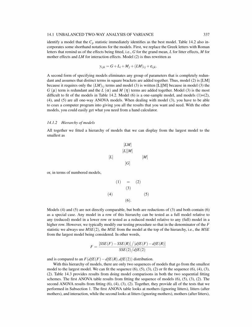
14.1.2 Hierarchy of models
All together we fitted a hierarchy of models that we can display from the largest model to thesmallest as
[LM]
[L][M]
[L] [M]
[G]
or, in terms of numbered models,
(1) = (2)(3)
(4) (5)(6).
Models (4) and (5) are not directly comparable, but both are reductions of (3) and both contain (6)as a special case. Any model in a row of this hierarchy can be tested as a full model relative toany (reduced) model in a lower row or tested as a reduced model relative to any (full) model in ahigher row. However, we typically modify our testing procedure so that in the denominator of the Fstatistic we always use MSE(2), the MSE from the model at the top of the hierarchy, i.e., the MSEfrom the largest model being considered. In other words,
F =[SSE(F)−SSE(R)]
/[dfE(F)−dfE(R)]
SSE(2)/
dfE(2)
and is compared to an F(dfE(F)−dfE(R),dfE(2)) distribution.With this hierarchy of models, there are only two sequences of models that go from the smallest
model to the largest model. We can fit the sequence (6), (5), (3), (2) or fit the sequence (6), (4), (3),(2). Table 14.3 provides results from doing model comparisons in both the two sequential fittingschemes. The first ANOVA table results from fitting the sequence of models (6), (5), (3), (2). Thesecond ANOVA results from fitting (6), (4), (3), (2). Together, they provide all of the tests that weperformed in Subsection 1. The first ANOVA table looks at mothers (ignoring litters), litters (aftermothers), and interaction, while the second looks at litters (ignoring mothers), mothers (after litters),

338 14. TWO-WAY ANOVA
Table 14.3: Analyses of variance for rat weight gains.
Source df Seq SS MS F PMothers 3 771.61 257.20 4.74 0.006Litters 3 63.63 21.21 0.39 0.761Mothers∗litters 9 824.07 91.56 1.69 0.120Error 45 2440.82 54.24Total 60 4100.13
Source df Seq SS MS F PLitters 3 60.16 20.05 0.37 0.776Mothers 3 775.08 258.36 4.76 0.006Litters∗mothers 9 824.07 91.56 1.69 0.120Error 45 2440.82 54.24Total 60 4100.13
and interaction. In the first ANOVA table, mothers are fitted to the data before litters. In the secondtable, litters are fitted before mothers.
Although models are fitted from smallest to largest and, in ANOVA tables, results are reportedfrom smallest model to largest, a sequence of models is evaluated from largest model to smallest.Thus, we begin the analysis of Table 14.3 at the bottom, looking for interaction. The rows formother∗litter interaction are identical in both tables. The sum of squares and degrees of freedomfor mother∗litter interaction in the table is obtained by differencing the error sums of squares anddegrees of freedom for models (3) and (2). If the interaction is significant, there is little point inlooking at the rest of the ANOVA table. One can either analyze the data as a one-way ANOVA ortry to model the interaction by developing models intermediate between models (2) and (3), cf.Subsection 15.3.2.
Our interaction F statistic is quite small, so there is little evidence of interaction and we proceedwith an analysis of model (3). In particular, we now examine the main effects. Table 14.3 showsclear effects for both mothers ignoring litters (F = 4.74) and mothers after fitting litters (F = 4.76)with little evidence for litters fitted after mothers (F = 0.39) or litters ignoring mothers (F = 0.37).
The difference in the error sums of squares for models (4) [L] and (3) [L][M] is the sum ofsquares reported for mothers in the second of the two ANOVA tables in Table 14.3. The differencein the error sums of squares for models (6) [G] and (5) [M] is the sum of squares reported formothers in the first of the two ANOVA tables in Table 14.3. The difference in the error sums ofsquares for models (5) [M] and (3) [L][M] is the sum of squares reported for litters in the first of thetwo ANOVA tables in Table 14.3. The difference in the error sums of squares for models (6) [G] and(4) [L] is the sum of squares reported for litters in the second of the ANOVA tables in Table 14.3.
Balanced two-way ANOVA is the special case where Ni j = N for all i and j. For balancedANOVA the two ANOVA tables (cf., Table 14.3) would be identical.
14.1.3 Computing issues
Many computer programs for fitting general linear models readily provide the ANOVA tables inTable 14.3. Recall that the interaction model (2) was written
yi jk = µ +αi +η j + γi j + εi jk
where µ is an overall effect (grand mean), the αis are effects for litter genotype, the η js are effectsfor foster mother genotype, and the γi js are effects for each combination of a litter genotype andfoster mother genotype. Just like regression programs, general linear models programs typically fita sequence of models where the sequence is determined by the order in which the terms are specified.Thus, specifying model (2) causes the sequence (6), (4), (3), (2) to be fitted and the second ANOVA

14.1 UNBALANCED TWO-WAY ANALYSIS OF VARIANCE 339
table in Table 14.3 to be produced. Specifying the equivalent but reordered model
yi jk = µ +η j +αi + γi j + εi jk
causes the sequence (6), (5), (3), (2) to be fitted and the first ANOVA table in Table 14.3 to beproduced.
When obtaining an analysis of model (2), many computer programs give ANOVA tables witheither the sequential sums of squares or “adjusted” sums of squares. Adjusted sums of squares arefor adding a term to the model last. Thus, in model (2) the adjusted sums of squares for Litters isthe sum of squares for dropping Litters out of the model
yi jk = µ +η j + γi j +αi + εi jk.
This is idiotic! As we have mentioned, the γi j terms can explain anything the αi or η j terms canexplain, so the model without litter main effects
yi jk = µ +η j + γi j + εi jk
is equivalent to model (2).What do these adjusted sums of squares really mean? Unfortunately, you have to enter the bow-
els of the computer program to find out. Most computer programs build in side conditions that allowthem to give some form of parameter estimates. Only model (1) really allows all the parameters tobe estimated. In any of the other models, parameters cannot be estimated without imposing somearbitrary side conditions. In the interaction model (2) the adjusted sums of squares for main effectsdepend on these side conditions, so programs that use different side conditions (and programs douse different side conditions), give different adjusted sums of squares for main effects after interac-tion. These values are worthless! Unfortunately, many programs, by default, produce mean squares,F statistics, and P values using these adjusted sums of squares. The interaction sum of squares andF test are not affected by this issue.
To be fair, if you are dealing with model (3) instead of model (2), the adjusted sums of squaresare perfectly reasonable. In model (3),
yi jk = µ +αi +η j + εi jk,
the adjusted sum of squares for Litters just compares model (3) to model (5) and the adjusted sum ofsquares for Mothers compares model (3) to model (4). Adjusted sums of squares are only worthlesswhen you fit main effects after having already fit an interaction that involves the main effect.
14.1.4 Discussion of model fitting
If there is no interaction but an effect for mothers after accounting for litters and an effect for littersafter accounting for mothers, both mothers and litters would have to appear in the final model, i.e.,
yi jk = µ +αi +η j + εi jk,
because neither effect could be dropped.If there were an effect for mothers after accounting for litters but no effect for litters after ac-
counting for mothers we could drop the effect of litters from the model. Then if the effect for motherswas still apparent when litters were ignored, a final model
yi jk = µ +αi + εi jk
that includes mother effects but not litter effects would be appropriate. Similar reasoning with theroles of mothers and litters reversed would lead one to the model
yi jk = µ +η j + εi jk.

340 14. TWO-WAY ANOVA
Unfortunately, except in special cases, it is possible to get contradictory results. If there were aneffect for mothers after accounting for litters but no effect for litters after accounting for motherswe could drop the effect of litters from the model and consider the model
yi jk = µ +αi + εi jk.
However, it is possible that in this model there may be no apparent effect for mothers (when littersare ignored), so dropping mothers is suggested and we get the model
yi jk = µ + εi jk.
This model contradicts our first conclusion that there is an effect for mothers, albeit one that onlyshows up after adjusting for litters. These issues are discussed more extensively in Christensen(2011, Section 7.5).
14.1.5 Diagnostics
It is necessary to consider the validity of our assumptions. Table 14.4 contains many of the standarddiagnostic statistics used in regression analysis. They are computed from the interaction model(2). Model (2) is equivalent to a one-way ANOVA model, so the leverage associated with yi jk inTable 14.3 is just 1/Ni j.
Figures 14.1 and 14.2 contain diagnostic plots. Figure 14.1 contains a normal plot of the stan-dardized residuals, a plot of the standardized residuals versus the fitted values, and boxplots of theresiduals versus Litters and Mothers, respectively. Figure 14.2 plots the leverages, the t residuals,and Cook’s distances against case numbers. The plots identify one potential outlier. From Table 14.3this is easily identified as the observed value of 68.0 for Litter I and Foster Mother A. This case hasby far the largest standardized residual r, standardized deleted residual t, and Cook’s distance C. Wecan test whether this case is consistent with the other data. The t residual of 4.02 has an unadjustedP value of 0.000225. If we use a Bonferroni adjustment for having made n = 61 tests, the P value is61×0.000225 .
= 0.014. There is substantial evidence that this case does not belong with the otherdata.
14.1.6 Outlier deleted analysis
We now consider the results of an analysis with the outlier deleted. Fitting the interaction model (2)we get
dfE(2) = 44, SSE(2) = 1785.60, MSE(2) = 40.58
and fitting the additive model (3) gives
dfE(3) = 53, SSE(3) = 3049,
so
Fobs =1263.48/9
40.58=
140.3940.58
= 3.46.
with a one-sided P value of .003. The interaction in significant, so we could reasonably go back totreating the data as a one-way ANOVA with 16 groups. Typically, we would print out the 16 groupmeans and try to figure out what is going on. But in this case, most of the story is determined by theplot of the standardized residuals versus the fitted values for the deleted data, Figure 14.3
Case 12 was dropped from the Litter I, Mother A group that contained three observations. Afterdropping case 12, that group has two observations and as can been seen from Figure 14.7, thatgroup has a far lower sample mean and has far less variability than any other group. In this example,deleting the one observation that does not seem consistent with the other data, makes the entiregroup inconsistent with the rest of the data.

14.1 UNBALANCED TWO-WAY ANALYSIS OF VARIANCE 341
Table 14.4: Diagnostics for rat weight gains: Model (14.1.2).
Case Litter Mother y y Leverage r t C1 A A 61.5 63.680 0.20 −0.33 −0.33 0.0022 A A 68.2 63.680 0.20 0.69 0.68 0.0073 A A 64.0 63.680 0.20 0.05 0.04 0.0004 A A 65.0 63.680 0.20 0.20 0.20 0.0015 A A 59.7 63.680 0.20 −0.60 −0.60 0.0066 F A 60.3 52.325 0.25 1.25 1.26 0.0337 F A 51.7 52.325 0.25 −0.10 −0.10 0.0008 F A 49.3 52.325 0.25 −0.47 −0.47 0.0059 F A 48.0 52.325 0.25 −0.68 −0.67 0.01010 I A 37.0 47.100 0.33 −1.68 −1.72 0.08811 I A 36.3 47.100 0.33 −1.89 −1.84 0.10112 I A 68.0 47.100 0.33 3.48 4.02 0.37713 J A 59.0 54.350 0.25 0.73 0.73 0.01114 J A 57.4 54.350 0.25 0.48 0.47 0.00515 J A 54.0 54.350 0.25 −0.05 −0.05 0.00016 J A 47.0 54.350 0.25 −1.15 −1.16 0.02817 A F 55.0 52.400 0.33 0.43 0.43 0.00618 A F 42.0 52.400 0.33 −1.73 −1.77 0.09319 A F 60.2 52.400 0.33 1.30 1.31 0.05320 F F 50.8 60.640 0.20 −1.49 −1.52 0.03521 F F 64.7 60.640 0.20 0.62 0.61 0.00622 F F 61.7 60.640 0.20 0.16 0.16 0.00023 F F 64.0 60.640 0.20 0.51 0.51 0.00424 F F 62.0 60.640 0.20 0.21 0.20 0.00125 I F 56.3 64.367 0.33 −1.34 −1.35 0.05626 I F 69.8 64.367 0.33 0.90 0.90 0.02627 I F 67.0 64.367 0.33 0.44 0.43 0.00628 J F 59.5 56.100 0.33 0.57 0.56 0.01029 J F 52.8 56.100 0.33 −0.55 −0.54 0.00930 J F 56.0 56.100 0.33 −0.02 −0.02 0.00031 A I 52.5 54.125 0.25 −0.25 −0.25 0.00132 A I 61.8 54.125 0.25 1.20 1.21 0.03033 A I 49.5 54.125 0.25 −0.73 −0.72 0.01134 A I 52.7 54.125 0.25 −0.22 −0.22 0.00135 F I 56.5 53.925 0.25 0.40 0.49 0.00336 F I 59.0 53.925 0.25 0.80 0.79 0.01337 F I 47.2 53.925 0.25 −1.05 −1.06 0.02338 F I 53.0 53.925 0.25 −0.15 −0.14 0.00039 I I 39.7 51.600 0.20 −1.81 −1.85 0.05140 I I 46.0 51.600 0.20 −0.85 −0.85 0.01141 I I 61.3 51.600 0.20 1.47 1.49 0.03442 I I 55.3 51.600 0.20 0.56 0.56 0.00543 I I 55.7 51.600 0.20 0.62 0.62 0.00644 J I 45.2 54.533 0.33 −1.55 −1.58 0.07545 J I 57.0 54.533 0.33 0.41 0.41 0.00546 J I 61.4 54.533 0.33 1.14 1.15 0.04147 A J 42.0 48.960 0.20 −1.06 −1.06 0.01748 A J 54.0 48.960 0.20 0.77 0.76 0.00949 A J 61.0 48.960 0.20 1.83 1.88 0.05250 A J 48.2 48.960 0.20 −0.12 −0.11 0.00051 A J 39.6 48.960 0.20 −1.42 −1.44 0.03252 F J 51.3 45.900 0.50 1.04 1.04 0.06753 F J 40.5 45.900 0.50 −1.04 −1.04 0.06754 I J 50.0 49.433 0.33 0.09 0.09 0.00055 I J 43.8 49.433 0.33 −0.94 −0.94 0.02756 I J 54.5 49.433 0.33 0.84 0.84 0.02257 J J 44.8 49.060 0.20 −0.65 −0.64 0.00758 J J 51.5 49.060 0.20 0.37 0.37 0.00259 J J 53.0 49.060 0.20 0.60 0.59 0.00660 J J 42.0 49.060 0.20 −1.07 −1.07 0.01861 J J 54.0 49.060 0.20 0.75 0.75 0.009

342 14. TWO-WAY ANOVA
−2 −1 0 1 2
−2−1
01
23
Normal Q−Q Plot
Theoretical Quantiles
Stan
dard
ized r
esidu
als
50 55 60 65
−2−1
01
23
Residual−Fitted plot
Fitted
Stan
dard
ized r
esidu
als
A F I J
−2−1
01
23
Residual−Litters plot
Litters
Stan
dard
ized r
esidu
als
A F I J
−2−1
01
23
Residual−Mothers plot
Mothers
Stan
dard
ized r
esidu
als
Figure 14.1: Residual plots for rat weight data. W ′ = 0.960.
0 10 20 30 40 50 60
0.20
0.30
0.40
0.50
Leverage index plot
i
Leve
rage
0 10 20 30 40 50 60
−2−1
01
23
4
t residual indexplot
i
rstud
ent(c
r)
0 10 20 30 40 50 60
0.00.1
0.20.3
Cook’s distance index plot
i
cook
s.dist
ance
(cr)
Figure 14.2: Diagnostic index plots for rat weight data.
The small mean value for the Litter I, Mother A group after deleting case 12 is causing theinteraction. If we delete the entire group, the interaction test becomes
Fobs =578.74/8
1785.36/43= 1.74 (14.1.7)
which gives a P value of .117. Note that by dropping the Litter I, Mother A group we go fromour original 61 observations to 58 observations, but we also go from 16 groups to 15 groups, sodfE(2) = 58−15= 43. On the other hand, the number of free parameters in model (3) is unchanged,so dfE(3) = 58−7 = 51, which leaves us 8 degrees of freedom in the numerator of the test.
14.1 UNBALANCED TWO-WAY ANALYSIS OF VARIANCE 343
40 45 50 55 60 65
−2−1
01
2
Residual−Fitted plot
Fitted
Stan
dard
ized r
esidu
als
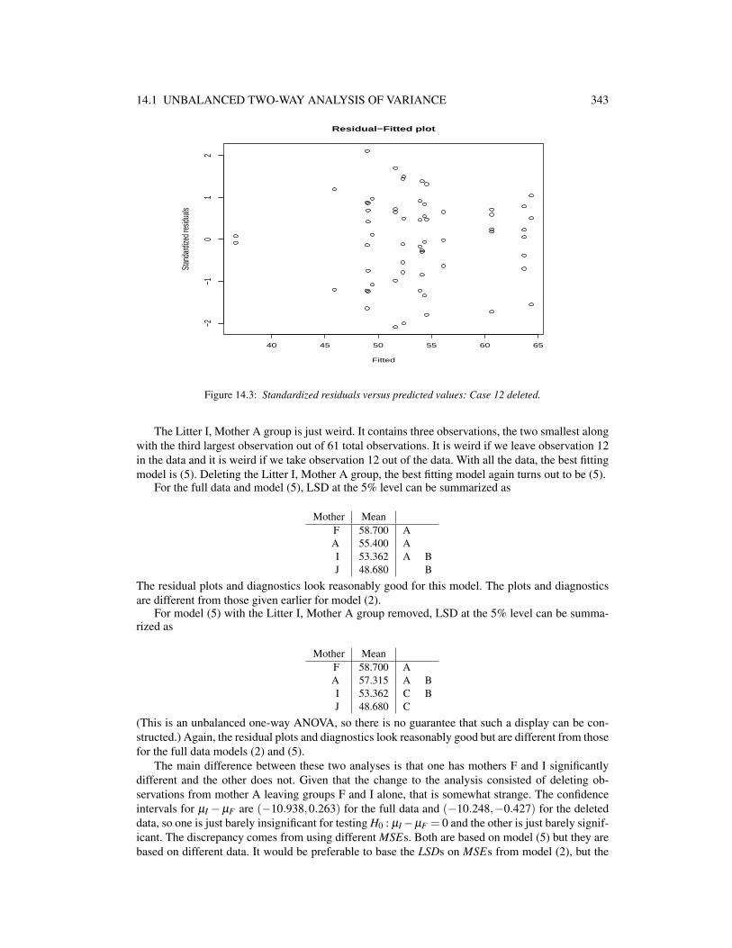
Figure 14.3: Standardized residuals versus predicted values: Case 12 deleted.
The Litter I, Mother A group is just weird. It contains three observations, the two smallest alongwith the third largest observation out of 61 total observations. It is weird if we leave observation 12in the data and it is weird if we take observation 12 out of the data. With all the data, the best fittingmodel is (5). Deleting the Litter I, Mother A group, the best fitting model again turns out to be (5).
For the full data and model (5), LSD at the 5% level can be summarized as
Mother MeanF 58.700 AA 55.400 AI 53.362 A BJ 48.680 B
The residual plots and diagnostics look reasonably good for this model. The plots and diagnosticsare different from those given earlier for model (2).
For model (5) with the Litter I, Mother A group removed, LSD at the 5% level can be summa-rized as
Mother MeanF 58.700 AA 57.315 A BI 53.362 C BJ 48.680 C
(This is an unbalanced one-way ANOVA, so there is no guarantee that such a display can be con-structed.) Again, the residual plots and diagnostics look reasonably good but are different from thosefor the full data models (2) and (5).
The main difference between these two analyses is that one has mothers F and I significantlydifferent and the other does not. Given that the change to the analysis consisted of deleting ob-servations from mother A leaving groups F and I alone, that is somewhat strange. The confidenceintervals for µI − µF are (−10.938,0.263) for the full data and (−10.248,−0.427) for the deleteddata, so one is just barely insignificant for testing H0 : µI −µF = 0 and the other is just barely signif-icant. The discrepancy comes from using different MSEs. Both are based on model (5) but they arebased on different data. It would be preferable to base the LSDs on MSEs from model (2), but the

344 14. TWO-WAY ANOVA
results would still be different for the different data. For all of the weirdness of the Litter I, MotherA group, in the end, the results are remarkably consistent whether we delete the group or not.
Finally, we have enough information to test whether the three observations in the Litter I, MotherA group are collectively a group of outliers. We do that by testing a full model that is model (2)defined for the deleted data against a reduced model that is model (2) for the full data. This mayseem like a backwards definition of a full and reduced model, but the deleted data version of model(2) can be obtained from the full data model (2) by adding a separate parameter for each of the threepoints we want to delete. Using information from equation (7) and either of Table 14.2 or 14.3,
Fobs =[2440.82−1785.36]/[45−43]
1785.36/43= 7.89,
which is highly significant: statistical evidence that Litter I, Mother A is a weird group. The numer-ator degrees of freedom is 2. Model (2) for the full data already has one parameter for the Litter I,Mother A group, so we need add only two more free parameters to have a separate parameter forevery observation in the group.
Minitab commands
The rat data are contained in Table 14.1. An appropriate data file might look like the first fourcolumns of Table 14.4 and we use C1, C2, C3, and C4 to indicate those columns. Below are Minitabcommands for the initial analysis of variance and the ANOVA tables in Table 14.1.MTB > names c1 ’Index" c2 ’Litters’ c3 ’Mothers’ c4 ’Weight’
MTB > glm c4 = c2|c3;
SUBC> fits c5;
SUBC> sresid c6;
SUBC> cookd c7;
SUBC> hi c8;
SUBC> tresid c9.
MTB > glm c4 = c3|c2;
In the ‘glm’ command, c2|c3 could be replaced by c2 c3 c2∗ c3. The c2 and c3 terms indicate maineffects for Litters and Mothers, respectively. Litter by Mother interaction is indicated by c2∗ c3.
Minitab’s glm command reports both sequential and adjusted sums of squares for each effectand by default performs tests with the adjusted sums of squares. This should be changed in the“Options” menu, especially when fitting interaction. The adjusted tests for main effects in modelsthat contain interaction are just silly. Adjusted tests are for fitting a term last, and the main effects addnothing to a model that already contains the “interaction” parameters. The reported tests depend onthe peccadillos of the programming. We have reported and analyzed the sequential sums of squares.
To delete the outlier in Minitab, just replace the 68.0 for case 12 with an asterisk (∗) and repeatthe commands given above.
14.2 Modeling contrasts
The interesting part of any analysis is figuring out how the groups really differ. To do that, you needto look at contrasts. We examined contrasts for one-way ANOVA models in Chapter 12, and all themodels we have looked at in this chapter, except the additive effects model, have been essentiallyone-way ANOVA models. In particular, our final conclusions about Mothers in the previous sectioncame from the one-way ANOVA that ignored Litters.
But what if we could not ignore litters? What if we needed to see how mothers differed in theadditive effects model rather than a one-way ANOVA? As mentioned earlier, when dealing with theadditive effects model you cannot just compute what you want on a hand calculator. You have to beable to coax whatever information you need out of a computer program. These issues are addressed

14.2 MODELING CONTRASTS 345
in this section and the next. You can generally get everything you need by fitting equivalent modelsin a regression program as discussed in the next section. Here we focus on extracting informationfrom an ANOVA program, i.e., we focus on manipulating the subscripts that are fed into an ANOVAprogram.
When the treatments have no structure to exploit, one way to start is by looking for evidence ofdifferences between all pairs of means.
BonferroniParameter Est SE(Est) t PηF −ηA 3.516 2.862 1.229 1.0000ηI −ηA −1.832 2.767 −0.662 1.0000ηJ −ηA −6.755 2.810 −2.404 0.1182ηI −ηF −5.35 2.863 −1.868 0.4029ηJ −ηF −10.27 2.945 −3.488 0.0059ηJ −ηI −4.923 2.835 −1.736 0.5293
If there are b levels of the second factor, as there are 4 levels of mother, there are b(b− 1)/2 =4(3)/2 = 6 pairwise comparisons to make. Of these, we will see in the next section that we can getb−1 = 4−1 = 3 of them by fitting a regression model. Some programs, like Minitab will provideall of the comparisons.
It is tempting to just summarize these results and be done with them. For an LSD procedure withα = .05 (actually specified as a Bonferonni procedure with α = .3), these results can be summarizedby
Mother MeanF 58.8 AA 55.2 AI 53.4 A BJ 48.5 B
It is by no means clear what the “Mean” values are. (They are explained in the next section.) Butwhat is important, and is reported correctly, are the relative differences among the “Mean” values.From the display, we see no differences among mothers F, A, and I and no difference betweenmothers I and J. We do see differences between F and J and between A and J.
Unfortunately, as discussed in Chapter 13, it is possible that no such display can be generated be-cause it is possible to have, say, a significant difference between F and A but no significant differencebetween F and I. This is possible, for example, if SE(ηF − ηA) is much smaller than SE(ηF − ηI).
Based on the pairwise testing results, one could perform a backwards elimination. The pair ofmeans with the least evidence for a difference from 0 is ηI −ηA with tobs = −0.662. We couldincorporate the assumption ηI = ηA into the model and look for differences between the remainingthree groups: mothers F, mothers J, and the combined group mothers A or I and continue the processof finding groups that could be combined. If we followed this procedure, at the next step we wouldcombine mothers A, F and I and then finally conclude that J was different from the other three.Another plausible model might be to combine J with A and I and leave F separate. These additivemodels with ηA = ηI , ηA = ηI = ηF , and ηA = ηI = ηJ have respective Cp values of 11.7, 13.2, and16.0. Only ηA = ηI is a minor improvement over the full two-factor additive effects model whichhas Cp = 13.2 as reported in Table 14.2.
The other methods of Section 12.4 extend easily to two-factor models but the results depend onthe specific model in which we incorporate the hypotheses.
14.2.1 Nonequivalence of tests
The general rule for unbalanced data is that if you change anything about a model you changeeverything about the model. We illustrate this by showing that the tests for ηF = ηA change betweenthe one-way model (14.1.5), the additive two-way model (14.1.3), and model (14.1.3) with the

346 14. TWO-WAY ANOVA
additional assumption that ηJ = ηI , even when we use the same denominator for all three F tests,namely the MSE from the interaction model (14.1.2).
The pairwise comparison estimates are determined as though the parameter is the last thing beingadded to the model. If we assumed that ηJ −ηI = 0, it could effect the estimate of the completelyunrelated parameter ηF −ηA, something that does not happen in one-way ANOVA. In fact, we willshow that for the rat data the test for ηF = ηA in the additive effects model is different dependingon whether you assume ηJ = ηI . First we illustrate that the test depends on whether or not we keeplitters in the model.
Assuming that there is no interaction, we might want to test that mothers A and F have the sameeffect, i.e., ηA = ηF or η1 = η2. We can incorporate this hypothesis into either the additive model(14.1.3) or the mothers only model (14.1.5). As is good practice, our tests will all use the MSE frommodel (14.1.2).
To incorporate ηA = ηF , when using a data file like the first four columns of Table 14.4, wemerely change the Mother column so that it contains the same symbol for mothers A and F. I justchanged all the Fs to As. Now we refit models (14.1.3) and (14.1.5) using this new “subscript” forthe Mothers.
Refitting the one-way model (14.1.5) incorporating ηA = ηF leads to the ANOVA tableAnalysis of Variance
Source df SS MS F PMother A=F 2 690.29 345.15 5.87 0.005Error 58 3409.83 58.79Total 60 4100.13
Using results from Table 14.2, to test ηA = ηF in model (14.1.5) the statistic is
Fobs =[3409.83−3328.52]/[58−57]
2440.82/45=
81.3154.24
= 1.50,
so the data are consistent with ηA = ηF in model (14.1.5). If we used the MSE from model (14.1.5)rather than model (14.1.2), this would be equivalent to performing the LSD test as we did in Sub-section 14.1.5. The ANOVA table F test for Mother A=F suggests that even when treating MothersA and F as the same group, there remain noticeable differences in the three remaining groups: A=F,I, and J.
To test ηA = ηF in the additive effects model (14.1.3) we must refit the model incorporatingηA = ηF . As in Table 14.3, refitting could lead to either the ANOVA table
Analysis of VarianceSource df SS MS F PMother A=F 2 690.29 345.15 5.66 0.006Litter 3 53.69 17.90 0.29 0.830Error 55 3356.15 61.02Total 60 4100.13
orAnalysis of Variance
Source df SS MS F PLitter 3 60.16 20.05 0.33 0.805Mother A=F 2 683.82 341.91 5.60 0.006Error 55 3356.15 61.02Total 60 4100.13
All we really care about is the Error term, and that is the same in both tables. Using results fromTable 14.2, to test ηA = ηF in model (14.1.3) the statistic is
Fobs =[3356.15−3264.89]/[55−54]
2440.82/45=
91.2654.24
= 1.68,

14.3 REGRESSION MODELING 347
so the data are again consistent with ηA = ηF , but now the result is for model (14.1.3). The ANOVAtable F statistics for Mother A=F after fitting Litters (F = 5.60) suggests that even when treatingMothers A and F as the same group, there remain noticeable differences in the three remaininggroups: A=F, I, and J.
The key point is that, as expected, the two F statistics for testing ηA = ηF in models (14.1.5)and (14.1.3) are noticeably different (even using the same denominator). In the former, it is 1.50 andin the latter it is 1.68. Note however that if we modify the denominator of the test for model (14.1.3)by using its own MSE we get
Fobs =[3356.15−3264.89]/[55−54]
3264.89/54= 1.509 = (1.2286)2,
which agrees with the t test given earlier for ηF = ηA in model (14.1.3).Unlike the one-way model, in the two-way additive model even the test for ηA = ηF depends on
our assumptions about the other mother effects. To demonstrate, we show that the test for ηA = ηFchanges when we assume ηI = ηJ . Building ηI = ηJ into the additive model (14.1.4) yields anANOVA table
Analysis of VarianceSeq.
Source df SS MS F PLitter 3 60.16 20.05 0.32 0.811Mother I=J 2 592.81 296.41 4.73 0.013Error 55 3447.16 62.68Total 60 4100.13
Now, if we also incorporate our hypothesis ηA = ηF we get an ANOVA table
Analysis of VarianceSeq.
Source df SS MS F PLitter 3 60.16 20.05 0.32 0.813Mother A=F;I=J 1 505.27 505.27 8.00 0.006Error 56 3534.70 63.12Total 60 4100.13
Comparing the error terms and using our usual denominator gives a different F statistic for testingηA = ηF assuming ηI = ηJ in the additive model,
Fobs =[3534.70−3447.16]/[56−55]
2440.82/45=
87.5454.24
= 1.61,
rather than the 1.68 we got from the additive model without assuming that ηI = ηJ .In this example, the test statistics are noticeably, but not substantially, different. With other data,
the differences can be much more substantial.In a balanced ANOVA, the numerators for these three tests would all be identical and the only
differences in the tests would be due to alternative choices of a MSE for the denominator.
14.3 Regression modeling
The additive effects modelyi jk = µ +αi +η j + εi jk
is the only new model that we have considered in this chapter. All of the other models reduce tofitting a one-way ANOVA. If we create four indicator variables, say, x1,x2,x3,x4 for the four Litter

348 14. TWO-WAY ANOVA
categories and another four indicator variables, say, x5,x6,x7,x8 for the four Mother categories, wecan rewrite the additive model as
yi jk = µ +α1xi j1 +α2xi j2 +α3xi j3 +α4xi j4 +η1xi j5 +η2xi j6 +η3xi j7 +η4xi j8 + εi jk.
The model is overparameterized. This occurs largely because for any i j,
xi j1 + xi j2 + xi j3 + xi j4 = 1 = xi j5 + xi j6 + xi j7 + xi j8.
Also, associated with the grand mean µ is a predictor variable that always takes the value 1, say, x0 ≡1. To make a regression model out of the additive effects model we need to drop one variable fromtwo of the three sets of variables {x0}, {x1,x2,x3,x4}, {x5,x6,x7,x8}. We illustrate the proceduresby dropping two of the three variables, x0, x2 (the indicator for Litter F), and x8 (the indicator forMother J).
If we drop x2 and x8 the model becomes
yi jk = δ + γ1xi j1 + γ3xi j3 + γ4xi j4 +β1xi j5 +β2xi j6 +β3xi j7 + εi jk. (14.3.1)
In this model, the Litter F, Mother J group becomes a baseline group and
δ = µ +α2 +η4, γ1 = α1 −α2, γ3 = α3 −α2, γ4 = α4 −α2,
β1 = η1 −η4, β2 = η2 −η4, β3 = η3 −η4.
After fitting model (1), the Table of Coefficients gives immediate results for testing whether differ-ences exist between Mother J and each of Mothers A, F, and I. It also gives immediate results fortesting no difference between Litter F and each of Litters A, I, and J.
If we drop x0, x8 the model becomes
yi jk = γ1xi j1 + γ2xi j2 + γ3xi j3 + γ4xi j4 +β1xi j5 +β2xi j6 +β3xi j7 + εi jk
but now
γ1 = µ +α1 +η4, γ2 = µ +α2 +η4, γ3 = µ +α3 +η4, γ4 = µ +α4 +η4,
β1 = η1 −η4, β2 = η2 −η4, β3 = η3 −η4,
so the Table of Coefficients still gives immediate results for testing whether differences exist be-tween Mother J and Mothers A, F, and I.
If we drop x0, x2 the model becomes
yi jk = γ1xi j1 ++γ3xi j3 + γ4xi j4 +β1xi j5 +β2xi j6 +β3xi j7 +β4xi j8 + εi jk.
Now
β1 = µ +η1 +α2, β2 = µ +η2 +α2, β3 = µ +η3 +α2, β4 = µ +η4 +α2,
γ1 = α1 −α2, γ3 = α3 −α2, γ4 = α4 −α2.
The Table of Coefficients still gives immediate results for testing whether differences exist betweenLitter F and Litters A, I, and J.
To illustrate these claims, we fit model (1) to the rat data to obtain the following Table of Coef-ficients.

14.3 REGRESSION MODELING 349
Table of CoefficientsPredictor Est SE(Est) t PConstant (δ ) 48.129 2.867 16.79 0.000x1:L-A (γ1) 2.025 2.795 0.72 0.472x3:L-I (γ3) −0.628 2.912 −0.22 0.830x4:L-J (γ4) 0.004 2.886 0.00 0.999x5:M-A (β1) 6.755 2.810 2.40 0.020x6:M-F (β2) 10.271 2.945 3.49 0.001x7:M-I (β3) 4.923 2.835 1.74 0.088
If, for example, you ask Minitab’s GLM procedure to test all pairs of Mother effects using aBonferroni adjustment, you get the table reported earlier,
BonferroniParameter Est SE(Est) t PηF −ηA 3.516 2.862 1.229 1.0000ηI −ηA −1.832 2.767 −0.662 1.0000ηJ −ηA −6.755 2.810 −2.404 0.1182ηI −ηF −5.35 2.863 −1.868 0.4029ηJ −ηF −10.27 2.945 −3.488 0.0059ηJ −ηI −4.923 2.835 −1.736 0.5293
Note that the estimate, say, β2 = η2 − η4 = ηF − ηJ = 10.271 is the negative of the estimate ofηJ −ηF , that they have the same standard error, that the t statistics are the negatives of each other,and that the Bonferroni P values are 6 times larger than the Table of Coefficient P values. Similarresults hold for β1 = η1 −η4 = ηA −ηJ and β3 = η3 −η4 = ηI −ηJ .
A display of results familiar from one-way ANOVA is
Mother MeanF 58.8 AA 55.2 AI 53.4 A BJ 48.5 B
The problems with the presentation are that the column of Mean values has little meaning and thatno meaningful display may be possible because standard errors depend on the difference beingestimated. As for the Mean values, the relative differences among the Mother effects are portrayedcorrectly, but the actual numbers are arbitrary. The relative sizes of Mother effects must be thesame for any Litter, but there is nothing one could call an overall Mother effect. You could add anyconstant to each of these four Mean values and they would be just as meaningful.
To obtain these “Mean” values as given, fit the model
yi jk = δ + γ1(xi j1 − xi j4)+ γ2(xi j2 − xi j4)+ γ3(xi j3 − xi j4)
+β1(xi j7 − xi j8)+β2(xi j6 − xi j8)+β3(xi j7 − xi j8)+ εi jk (2)
to get the following Table of Coefficients.

350 14. TWO-WAY ANOVA
Table of CoefficientsPredictor Est SE(Est) t PConstant (δ ) 53.9664 0.9995 53.99 0.000LitterA (γ1) 1.675 1.675 1.00 0.322F (γ2) −0.350 1.763 −0.20 0.843I (γ3) −0.979 1.789 −0.55 0.587
MotherA (β1) 1.268 1.702 0.75 0.459F (β2) 4.784 1.795 2.66 0.010I (β3) −0.564 1.712 −0.33 0.743
The “Mean” values in the display are obtained from the Table of Coefficients, wherein the estimatedeffect for mother F is 58.8 = δ + β2 = 53.9664+4.784, for mother A is 55.2 = δ + β1 = 53.9664+1.268, for mother I is 53.4 = δ + β3 = 53.9664−0.564, and for mother J is 48.5 = δ − (β1 + β2 +
β3) = 53.9664− (1.268+4.784−0.564).Dropping two predictor variables is equivalent to imposing side conditions on the parameters.
Dropping x2 and x8 amounts to assuming α2 = 0 = η4. Dropping the intercept x0 and x8 amounts toassuming that µ = 0= η4. Dropping x0 and x2 amounts to assuming that µ = 0=α2. The regressionmodel (2) is equivalent to assuming that α1 +α2 +α3 +α4 = 0 = η1 +η2 +η3 +η4.
14.4 Homologous factors
An interesting aspect of having two factors is dealing with factors that have comparable levels. Forexample, the two factors could be mothers and fathers and the factor levels could be a categorizationof their educational level, perhaps: not a high school graduate, high school graduate, some college,college graduate, post graduate work. In addition to the issues raised already, we might be interestedin whether fathers’ education has the same effect as mothers’ education. Alternatively, the twofactors might be a nitrogen based fertilizer and a phosphorus based fertilizer and the levels might bemultiples of a standard dose. In that case we might be interested in whether nitrogen and phosphorushave the same effect. Factors with comparable levels are called homologous factors. Example 14.1.1involves genotypes of mothers and genotypes of litters where the genotypes are identical for themothers and the litters, so it provides an example of homologous factors.
14.4.1 Symmetric additive effects
We have talked about father’s and mother’s educational levels having the same effect. To do thiswe must have reasonable definitions of the effects for a father’s educational level and a mother’seducational level. As discussed in Section 1, factor level effects are well defined in the additivetwo-way model
yi jk = µ +αi +η j + ei jk. (14.4.1)
Here the αis represent, say, father’s education effects or litter genotype effects and the η js representmother’s education effects or foster mother genotype effects. Most often with homologous factorswe assume that the number of levels is the same for each factor. For the education example, fathersand mothers both have 5 levels. For the rat genotypes, both factors have 4 levels. We call this numbert. (Occasionally, we can extend these ideas to unequal numbers of levels.)
If fathers’ and mothers’ educations have the same effect, or if litters’ and foster mothers’ geno-types have the same effect, then
α1 = η1, . . . ,αt = ηt .
Incorporating this hypothesis into the additive effects model (1) gives the symmetric additive effectsmodel
yi jk = µ +αi +α j + ei jk (14.4.2)

14.4 HOMOLOGOUS FACTORS 351
Alas, not many ANOVA computer programs know how to fit such a model, so we will have to do itourselves in a regression program. The remainder of the discussion in this subsection is for the ratweight data.
We begin by recasting the additive effects model (1) as a regression model. The factor variableLitters has 4 levels, so, similar to Section 12.3, we can replace it with 4 indicator variables, say, LA,LF , LI , LJ . We can also replace the 4 level factor variable Mothers with 4 indicator variables, MA,MF , MI , MJ . Now the no interaction model (1) can be written
yh = µ +α1LhA +α2LhF +α3LhI +α4LhJ +η1MhA +η2MhF +η3MhI +η4MhJ + εh, (14.4.3)
h = 1, . . . ,61. This model is overparameterized. If we just run the model, most good regressionprograms are smart enough to throw out redundant parameters (predictor variables). Performingthis operation ourselves, we fit the model
yh = µ +α1LhA +α2LhF +α3LhI +η1MhA +η2MhF +η3MhI + εh (14.4.4)
that eliminates LJ and MJ . Remember, model (4) is equivalent to (1) and (3). Fitting model (4), wehave little interest in the Table of Coefficients but the ANOVA table follows.
Analysis of Variance: Model (14.4.4)Source df SS MS F PRegression 6 835.24 139.21 2.30 0.047Error 54 3264.89 60.46Total 60 4100.13
As advertised, the Error line agrees with the results given for the no interaction model (14.1.2) inSection 1.
To fit the symmetric additive effects model (2), we incorporate the assumption α1 =η1, . . . ,α4 =η4 into model (3) getting
yh = µ +α1LhA +α2LhF +α3LhI +α4LhJ +α1MhA +α2MhF +α3MhI +α4MhJ + εh
oryh = µ +α1(LhA +MhA)+α2(LhF +MhF)+α3(LhI +MhI)+α4(LhJ +MhJ)+ εh.
Fitting this model requires us to construct new regression variables, say,
A = LA +MA
F = LF +MF
I = LI +MI
J = LJ +MJ .
The symmetric additive effects model (2) is then written as
yh = µ +α1Ah +α2Fh +α3Ih +α4Jh + εh
or, emphasizing that the parameters mean different things,
yh = γ0 + γ1Ah + γ2Fh + γ3Ih + γ4Jh + εh.
This model is also overparameterized, so we actually fit
yh = γ0 + γ1Ah + γ2Fh + γ3Ih + εh, (14.4.5)
giving

352 14. TWO-WAY ANOVA
Table of Coefficients: Model (14.4.5)Predictor γk SE(µk) t PConstant 48.338 2.595 18.63 0.000A 4.159 1.970 2.11 0.039F 5.049 1.912 2.64 0.011I 1.998 1.927 1.04 0.304
andAnalysis of Variance: Model (14.4.5)
Source df SS MS F PRegression 3 513.64 171.21 2.72 0.053Error 57 3586.49 62.92Total 60 4100.13
We need the ANOVA table Error line to test whether the symmetric additive effects model (2)fits the data adequately relative to the additive effects model (1). The test statistic is
Fobs =[3586.49−3264.89]/[57−54]
60.46= 1.773
with P = 0.164, so the model seems to fit.Presuming that the symmetric additive effects model (4) fits, we can interpret the Table of Coef-
ficients. We dropped variable J in the model, so the constant term γ0 = 48.338 estimates the effectof having genotype J. The estimated regression coefficient for A, γ1 = 4.159, is the estimated effectfor the difference between the genotype A effect and the genotype J effect. The P value of 0.039 in-dicates weak evidence for a difference between genotypes A and J. Similarly, there is pretty strongevidence for a difference between genotypes F and J (P = 0.011) but little evidence for a differ-ence between genotypes I and J (P = 0.304). From the table of coefficients, the estimated effect forhaving, say, genotype A is 48.338+4.159 = 52.497.
As discussed in Section 1, it would be reasonable to use the interaction model MSE in thedenominator of the F statistic which makes
Fobs =[3586.49−3264.89]/[57−54]
54.24= 1.976,
but the P value remains a relatively high 0.131.
14.4.2 Skew symmetric additive effects
Thinking of parents education and genotypes, it is possible that fathers’ and mothers’ educationcould have exact opposite effects or that litters’ and mothers’ genortypes could have exact oppositeeffects, i.e.,
α1 =−η1, . . . ,αt =−ηt .
Incorporating this hypothesis into the additive effects model (1) gives the skew symmetric additiveeffects model
yi jk = µ +αi −α j + ei jk. (14.4.6)
Sometimes this is called the alternating additive effects model.In model (6), µ is a well defined parameter and it is the common mean value for the four
groups that have the same genotype for litters and mothers. The skew symmetric additive model isoverparameterized but only in that the αs are redundant.
To fit the model, we write it in regression form
yh = µ +α1(LhA −MhA)+α2(LhF −MhF)+α3(LhI −MhI)+α4(LhJ −MhJ)+ εh (14.4.7)
and drop the last predictor LJ −MJ .

14.4 HOMOLOGOUS FACTORS 353
Table of Coefficients: Model (14.4.7)Predictor γk SE(µk) t PConstant 53.999 1.048 51.54 0.000(LA −MA) −2.518 2.098 −1.20 0.235(LF −MF) −4.917 2.338 −2.10 0.040(LI −MI) −2.858 2.273 −1.26 0.214
Analysis of Variance: Model (14.4.7)Source df SS MS F PRegression 3 297.73 99.24 1.49 0.228Error 57 3802.39 66.71Total 60 4100.13
If the model fitted the data, we could interpret the table of coefficients. Relative to model (4), theparameter estimates are γ0 = µ , γ1 = α1 − α4 ≡ αA − αJ , γ2 = α3 − α4 ≡ αF − αJ , γ3 = α3 − α4 ≡αI − αJ . But the skew symmetric additive model does not fit very well because, relative to theadditive model (1),
Fobs =[3802.39−3264.89]/[57−54]
60.46= 2.93
which gives P = .042.It is of some interest to note that the model that includes both symmetric additive effects and
skew symmetric additive effects,
yh = µ +α1Ah +α2Fh +α3Ih +α4Jh + α1(LhA −MhA)
+ α2(LhF −MhF)+ α3(LhI −MhI)+ α4(LhJ −MhJ)+ εh
is actually equivalent to the no interaction model (1). Thus, our test for whether the symmetricadditive model fits can also be thought of as a test for whether skew symmetric additive effectsexist after fitting symmetric additive effects and our test for whether the skew symmetric additivemodel fits can also be thought of as a test for whether symmetric additive effects exist after fittingskew symmetric additive effects. Neither the symmetric additive model (2) nor the skew symmetricadditive model (6) is comparable to either of the single effects only models (14.1.4) and (14.1.5).
14.4.3 Symmetry
The assumption of symmetry is that the two factors are interchangeable. Think again about ourfathers’ and mothers’ education. Under symmetry, there is no difference between having a collegegraduate father and postgraduate mother as opposed to having a postgraduate father and collegegraduate mother. Symmetric additive models display this symmetry but impose the structure thatthere is some consistent effect for, say, being a college graduate and for being a high school graduate.But symmetry can exist even when no overall effects for educational levels exist. For overall effectsto exist, the effects must be additive.
Table 14.5 gives examples of symmetric additive and symmetric nonadditive effects. The sym-metric additive effects have a “grand mean” of 10, an effect of 0 for being less than a HS Grad, andeffect of 2 for a HS Grad, an effect of 3 for some college, and an effect of 5 for both college gradand postgrad. The nonadditive effects were obtained by modifying the symmetric additive effects.In the nonadditive effects any pair where both parents have any college is up 3 units and any pairwhere both parents are without any college is down 2 units.
In Subsection 14.4.1 we looked carefully at the symmetric additive effects model which is a spe-cial case of the additive effects (no interaction) model. Now we impose symmetry on the interactionmodel.
Rather than the interaction model (14.1.2) we focus on the equivalent one-way ANOVA model(14.1.1), i.e.,
yi jk = µi j + εi jk. (14.4.8)

354 14. TWO-WAY ANOVA
Table 14.5: Symmetric and symmetric additive education effects.
Symmetric Additive EffectsEduc. Level Education Level of Mother Fatherof Fathers <HS HS Grad <Coll Coll Grad Post Effect<HS 10 12 13 15 15 0
HS Grad 12 14 15 17 17 2<Coll 13 15 16 18 18 3
Coll Grad 15 17 18 20 20 5Post 15 17 18 20 20 5
Mother Effect 0 2 3 5 5Symmetric Nonadditive Effects
Educ. Level Education Level of Motherof Fathers <HS HS Grad <Coll Coll Grad Post<HS 8 10 13 15 15
HS Grad 10 12 15 17 17<Coll 13 15 19 21 21
Coll Grad 15 17 21 23 23Post 15 17 21 23 23
Table 14.6: Rat indices.
One-Way ANOVA: subscripts rGenotype of Genotype of Foster Mother
Litter A F I JA 1 5 9 13F 2 6 10 14I 3 7 11 15J 4 8 12 16
Symmetric group effects: subscripts sGenotype of Genotype of Foster Mother
Litter A F I JA 1 2 3 4F 2 6 7 8I 3 7 11 12J 4 8 12 16
For rat genotypes, i = 1, . . . ,4 and j = 1, . . . ,4 are used together to indicate the 16 groups. Alterna-tively, we can replace the pair of subscripts i j with a single subscript r = 1, . . . ,16,
yrk = µr + εrk. (14.4.9)
The top half of Table 14.6 shows how the subscripts r identify the 16 groups. The error for thismodel should agree with the error for model (14.1.2) which was given in Section 1. You can seefrom the ANOVA table that it does.
Analysis of Variance: Model (14.4.9)Source df SS MS F PRat groups 15 1659.3 110.6 2.04 0.033Error 45 2440.8 54.2Total 60 4100.1
To impose symmetry, in model (8) we require that for all i and j,
µi j = µ ji.
This places no restrictions on the four groups with i = j. Translating the symmetry restriction intomodel (9) with the identifications of Table 14.6, symmetry becomes
µ2 = µ5,µ3 = µ9,µ4 = µ13,µ7 = µ10,µ8 = µ14,µ12 = µ15.

14.4 HOMOLOGOUS FACTORS 355
Imposing these restrictions on the one-way ANOVA model (9) amounts to constructing a new one-way ANOVA model with only 10 groups. Symmetry forces the 6 pairs of groups for which i = j and(i, j) = ( j, i) to act like 6 single groups and the 4 groups with i = j are unaffected by symmetry. Thebottom half of Table 14.6 provides subscripts s for the one-way ANOVA model that incorporatessymmetry
ysm = µs + εsm. (14.4.10)
Note that in the nonadditive symmetry model (10), the second subscript for identifying observationswithin a group also has to change. There are still 61 observations, so if we use fewer groups, wemust have more observations in some groups.
Fitting the nonadditive symmetry model gives
Analysis of Variance: Model (14.4.10)Source df SS MS F Psymmetric groups 9 1159.4 128.8 2.23 0.034Error 51 2940.8 57.7Total 60 4100.1
Testing this against the interaction model (6) provides
Fobs =[2940.8−2440.8]/[51−45]
54.24= 1.54
with P = 0.188. The nonadditive symmetry model is consistent with the data.We can also test the symmetry model (10) versus the reduced symmetric additive effects model
(1) giving
Fobs =[3264.89−2940.8]/[54−51]
54.24= 1.99
with P = 0.129, so there is no particular reason to choose the nonadditive symmetry model over theadditive symmetry model.
Finally, it would also be possible to define a skew symmetry model. With respect to model (5)skew symmetry imposes
µi j =−µ ji,
which implies that µii = 0. To fit this model we would need to construct indicator variables for all16 groups, say I1, . . . , I16. From these we can construct both the symmetric model and the skewsymmetric model. Using the notation of the top half of Table 14.6, the symmetry model would have10 indicator variables
I1, I6, I11, I16, I2 + I5, I3 + I9, I4 + I13, I7 + I10, I8 + I14, I12 + I15.
The skew symmetric model would use the 6 predictor variables
I2 − I5, I3 − I9, I4 − I13, I7 − I10, I8 − I14, I12 − I15.
If we used all 16 of the predictor variables in the symmetry and skew symmetry model, we wouldhave a model equivalent to the interaction model (8), so the test for the adequacy of the symmetrymodel is also a test for whether skew symmetry adds anything after fitting symmetry.
It is hard to imagine good applications of skew symmetry. Perhaps less so if we added an inter-cept to the skew symmetry variables, since that would make it a generalization of the skew symmet-ric additive model. In fact, to analyze homologous factors without replications, i.e., when model (8)has 0 degrees of freedom for error, McCullagh (2000) suggests using the MSE from the symmetrymodel as a reasonable estimate of error, i.e., take as error the mean square for skew symmetry afterfitting symmetry.
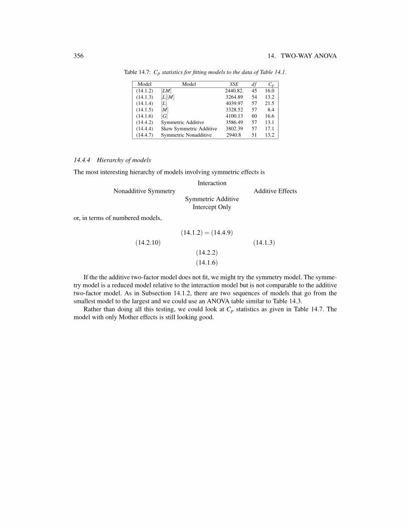
356 14. TWO-WAY ANOVA
Table 14.7: Cp statistics for fitting models to the data of Table 14.1.
Model Model SSE df Cp(14.1.2) [LM] 2440.82. 45 16.0(14.1.3) [L][M] 3264.89 54 13.2(14.1.4) [L] 4039.97 57 21.5(14.1.5) [M] 3328.52 57 8.4(14.1.6) [G] 4100.13 60 16.6(14.4.2) Symmetric Additive 3586.49 57 13.1(14.4.4) Skew Symmetric Additive 3802.39 57 17.1(14.4.7) Symmetric Nonadditive 2940.8 51 13.2
14.4.4 Hierarchy of models
The most interesting hierarchy of models involving symmetric effects is
InteractionNonadditive Symmetry Additive Effects
Symmetric AdditiveIntercept Only
or, in terms of numbered models,
(14.1.2) = (14.4.9)(14.2.10) (14.1.3)
(14.2.2)(14.1.6)
If the the additive two-factor model does not fit, we might try the symmetry model. The symme-try model is a reduced model relative to the interaction model but is not comparable to the additivetwo-factor model. As in Subsection 14.1.2, there are two sequences of models that go from thesmallest model to the largest and we could use an ANOVA table similar to Table 14.3.
Rather than doing all this testing, we could look at Cp statistics as given in Table 14.7. Themodel with only Mother effects is still looking good.