chapter 13 basic audio compression techniques…brahms.emu.edu.tr/babagil/10-comp306-basic audio...

Chapter 13 Basic Chapter 13 Basic Audio Audio Compression Compression Techniques Techniques 13 1 ADPCM in Speech Coding 13.1 ADPCM in Speech Coding 13.2 G.726 ADPCM 13.3 Vocoders 13 4 Further Exploration 13.4 Further Exploration

1

13 1 ADPCM in Speech Coding 13 1 ADPCM in Speech Coding 13.1 ADPCM in Speech Coding 13.1 ADPCM in Speech Coding

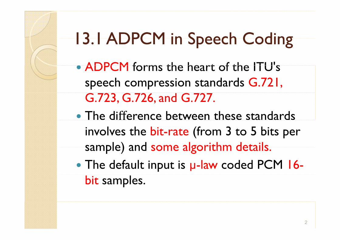
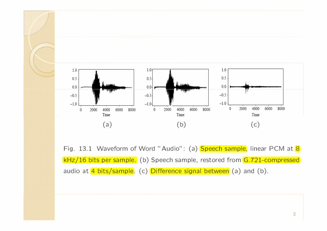
ADPCM forms the heart of the ITU's ADPCM forms the heart of the ITU s speech compression standards G.721, G.723, G.726, and G.727. The di erence between these standards involves the bit-rate (from 3 to 5 bits per sample) and some algorithm details sample) and some algorithm details. The default input is µ-law coded PCM 16-bit samples.

2

13 2 G 726 ADPCM 13 2 G 726 ADPCM 13.2 G.726 ADPCM 13.2 G.726 ADPCM

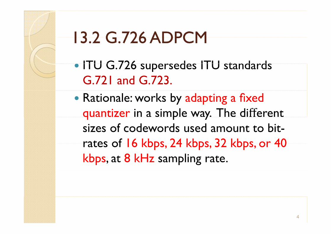
ITU G 726 supersedes ITU standards ITU G.726 supersedes ITU standards G.721 and G.723. Rationale: works by adapting a fixed quantizer in a simple way. The di erent q p ysizes of codewords used amount to bit-rates of 16 kbps 24 kbps 32 kbps or 40 rates of 16 kbps, 24 kbps, 32 kbps, or 40 kbps, at 8 kHz sampling rate.

4

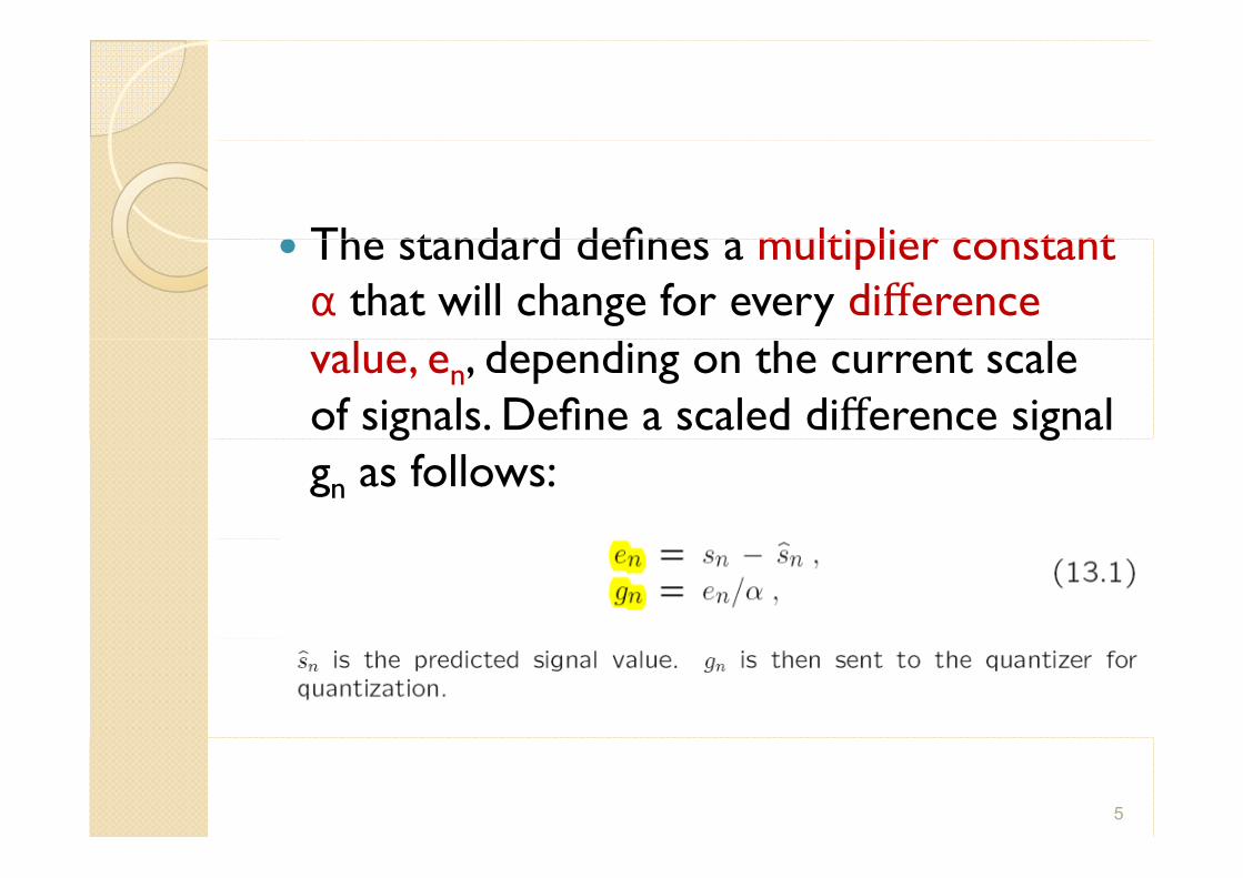
The standard defines a multiplier constant The standard defines a multiplier constant α that will change for every di erence value, en, depending on the current scale of signals. Define a scaled di erence signal g ggn as follows:

5

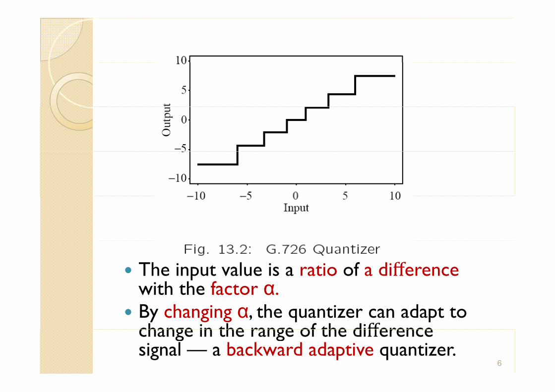
The input value is a ratio of a di erenceith th f t α with the factor α.

By changing α, the quantizer can adapt to change in the range of the di erencechange in the range of the di erencesignal — a backward adaptive quantizer.

6

Backward Adaptive Quantizer Backward Adaptive Quantizer Backward Adaptive Quantizer Backward Adaptive Quantizer Backward adaptive works in principle by noticing Backward adaptive works in principle by noticing either of the cases: ◦ too many values are quantized to values far from

ld h if i i i f zero – would happen if quantizer step size in f were too small. ◦ too many values fall close to zero too much of the y

time would happen if the quantizer step size were too large.

Jayant quantizer allows one to adapt a backward Jayant quantizer allows one to adapt a backward quantizer step size after receiving just one single output. ◦ Jayant quantizer simply expands the step size if the

quantized input is in the outer levels of the quantizer, and reduces the step size if the input is near zero. and reduces the step size if the input is near zero.

7

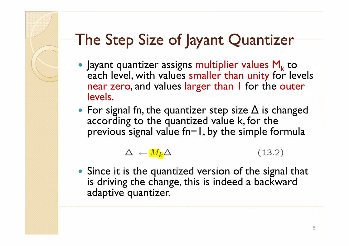
The Step Size of Jayant Quantizer The Step Size of Jayant Quantizer The Step Size of Jayant Quantizer The Step Size of Jayant Quantizer Jayant quantizer assigns multiplier values Mk to Jayant quantizer assigns multiplier values Mk to each level, with values smaller than unity for levels near zero, and values larger than 1 for the outer le els levels. For signal fn, the quantizer step size ∆ is changed according to the quantized value k, for the according to the quantized value k, for the previous signal value fn−1, by the simple formula

Since it is the quantized version of the signal that i d i i h h hi i i d d b k d is driving the change, this is indeed a backward adaptive quantizer.

8

G.726 G.726 —— Backward Adaptive Jayant Backward Adaptive Jayant Quantizer Quantizer

G.726 uses fixed quantizer steps based on the G.726 uses fixed quantizer steps based on the logarithm of the input difference signal, en divided by α. The divisor α is:

β ≡ log2 α (13 3) β ≡ log2 α (13.3)

When difference values are large α is divided into: When difference values are large, α is divided into: ◦ locked part αL – scale factor for small difference values. ◦ unlocked part αU — adapts quickly to larger differences. ◦ These correspond to log quantities βL and βU ,so that:

* A changes so that it is about unity, for speech, and about zero, for voice-band data.

9

The "unlocked" part adapts via the equationp p q

The locked part is slightly modified from the unlocked part: p g y p

The G.726 predictor is quite complicated: it uses a linear p q pcombination of 6 quantized differences and two reconstructed signal values, from the previous 6 signal values fn.

10

13 3 Vocoders 13 3 Vocoders 13.3 Vocoders 13.3 Vocoders Vocoders – voice coders which cannot be Vocoders voice coders, which cannot be usefully applied when other analog signals, such as modem signals, are in use. g◦ concerned with modeling speech so that the salient

features are captured in as few bits as possible. ◦ use either a model of the speech waveform in time

(LPC (Linear Predictive Coding) vocoding), or ... →◦ break down the signal into frequency components ◦ break down the signal into frequency components

and model these (channel vocoders and formant vocoders).

Vocoder simulation of the voice is not very good yet.

11

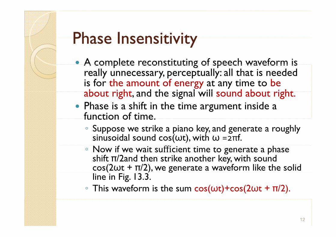
Phase Insensitivity Phase Insensitivity Phase Insensitivity Phase Insensitivity A complete reconstituting of speech waveform is A complete reconstituting of speech waveform is really unnecessary, perceptually: all that is needed is for the amount of energy at any time to be ab t ri ht and the si nal ill s nd ab t ri ht about right, and the signal will sound about right. Phase is a shift in the time argument inside a function of time. function of time. ◦ Suppose we strike a piano key, and generate a roughly

sinusoidal sound cos(ωt), with ω =2πf. ◦ Now if we wait sufficient time to generate a phase

shift π/2and then strike another key, with sound cos(2ωt + π/2), we generate a waveform like the solid ( ) gline in Fig. 13.3. ◦ This waveform is the sum cos(ωt)+cos(2ωt + π/2).

12

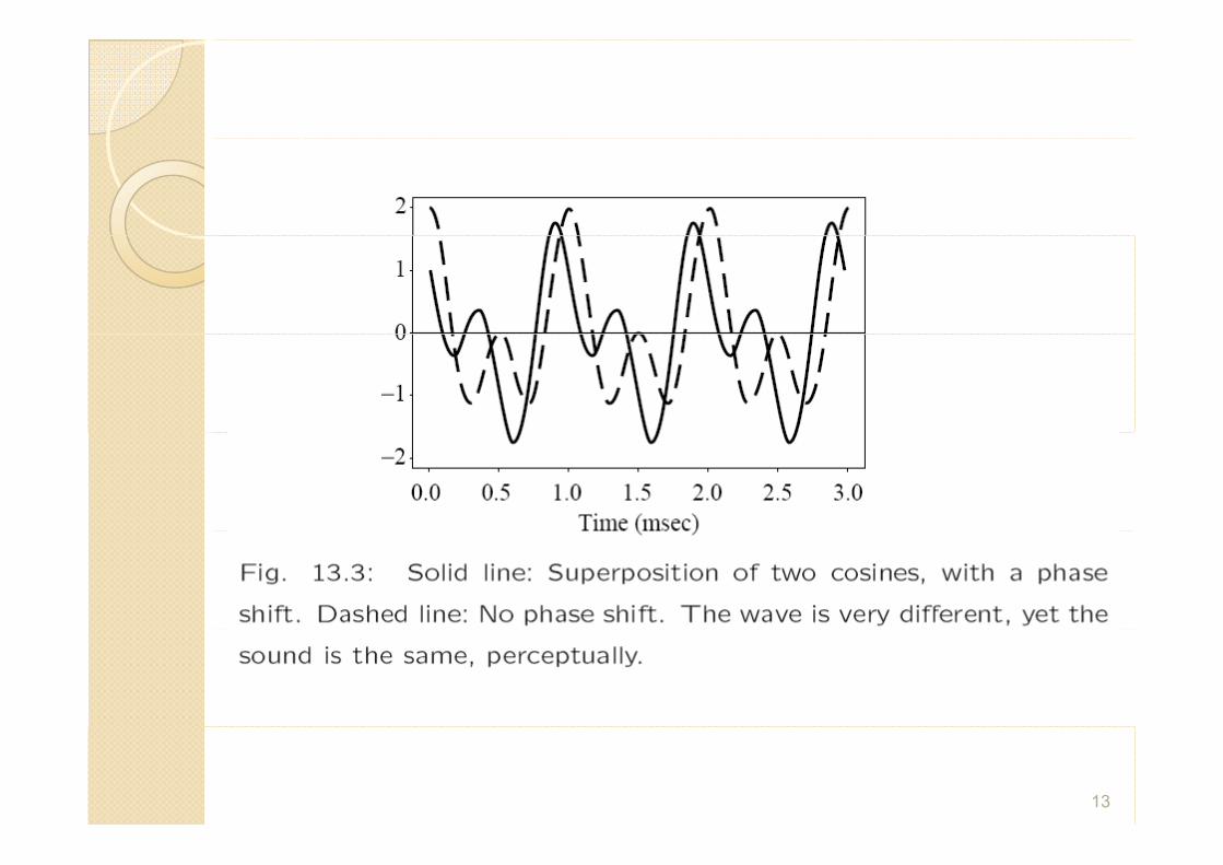
If we did not wait before striking the – If we did not wait before striking the second note, then our waveform would be cos(ωt)+cos(2ωt). But perceptually, the two notes would sound the same sound, even though in actuality they would be shifted in phase. would be shifted in phase.

13

Channel Vocoder Channel Vocoder Channel Vocoder Channel Vocoder Vocoders can operate at low bit-rates, 1–2 kbps. To Vocoders can operate at low bit rates, 1 2 kbps. To do so, a channel vocoder first applies a filter bank to separate out the different frequency components:

14

Due to Phase Insensitivity (i.e. only the energy is Due to Phase Insensitivity (i.e. only the energy is important): ◦ The waveform is "rectified" to its absolute value.

Th fil b k d i l i l l f h ◦ The filter bank derives relative power levels for each frequency range.

◦ A subband coder would not rectify the signal, and would id f b d use wider frequency bands.

A channel vocoder also analyzes the signal to determine the general pitch of the speech (low —g p p (bass, or high — tenor), and also the excitation of the speech. A channel vocoder applies a vocal tract transfer A channel vocoder applies a vocal tract transfer model to generate a vector of excitation parameters that describe a model of the sound, and also guesses

h h h d i i d i d whether the sound is voiced or unvoiced.

15

Formant Formant VocoderVocoderFormant Formant VocoderVocoderFormants: the salient frequency components that are Formants: the salient frequency components that are present in a sample of speech, as shown in Fig 13.5. Rationale: encoding only the most important frequencies frequencies.

16

Linear Predictive Coding (LPC) Linear Predictive Coding (LPC) Linear Predictive Coding (LPC) Linear Predictive Coding (LPC) LPC vocoders extract salient features of speech LPC vocoders extract salient features of speech directly from the waveform, rather than transforming the signal to the frequency domain LPC F LPC Features: ◦ uses a time-varying model of vocal tract sound

generated from a given excitation generated from a given excitation ◦ transmits only a set of parameters modeling the

shape and excitation of the vocal tract, not actual i l diff ll bit t signals or differences small bit-rate

About "Linear": The speech signal generated by the output vocal tract model is calculated as a the output vocal tract model is calculated as a function of the current speech output plus a second term linear in previous model coe cients

17

LPC Coding Process LPC Coding Process LPC Coding Process LPC Coding Process LPC starts by deciding whether the current LPC starts by deciding whether the current segment is voiced or unvoiced: ◦ For unvoiced: a wide-band noise generator is g

used to create sample values f(n) that act as input to the vocal tract simulator ◦ For voiced: a pulse train generator creates values ◦ For voiced: a pulse train generator creates values

f(n) ◦ Model parameters ai: calculated by using a least-p i y g

squares set of equations that minimize the di erence between the actual speech and the speech generated by the vocal tract model speech generated by the vocal tract model, excited by the noise or pulse train generators that capture speech parameters

18

LPC Coding Process (cont'd) LPC Coding Process (cont'd) LPC Coding Process (cont d) LPC Coding Process (cont d)

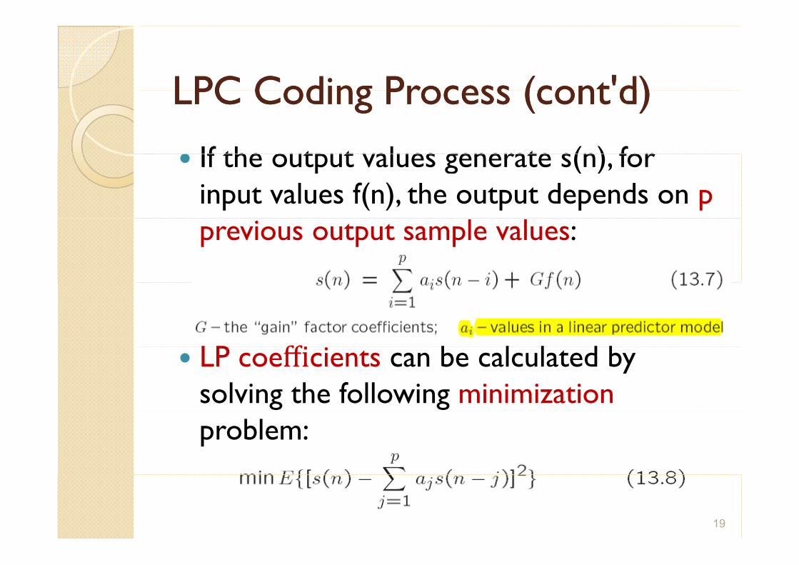
If the output values generate s(n) for If the output values generate s(n), for input values f(n), the output depends on p previous output sample values:

LP b l l d b LP coe cients can be calculated by solving the following minimization problem:

19


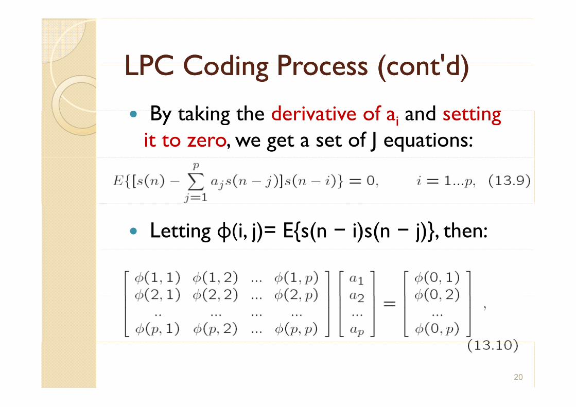
By taking the derivative of a and setting By taking the derivative of ai and setting it to zero, we get a set of J equations:

Letting φ(i, j)= E{s(n − i)s(n − j)}, then:

20


An often used method to calculate LP An often-used method to calculate LP coefficients is the autocorrelation method:

21

LPC Coding Process (cont'd) LPC Coding Process (cont'd) LPC Coding Process (cont d) LPC Coding Process (cont d) Since φ(i j) can be defined as φ(i j)= R(|i −Since φ(i, j) can be defined as φ(i, j) R(|ij|), and when R(0) ≥ 0, the matrix {φ(i, j)} is positive symmetric, there exists a fast p yscheme to calculate the LP coe cients:

22


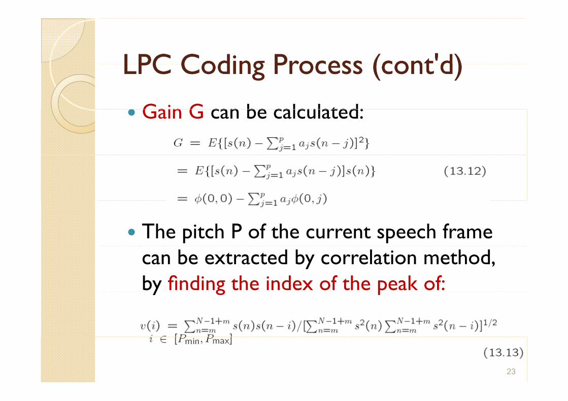
Gain G can be calculated: Gain G can be calculated:

The pitch P of the current speech frame can be extracted by correlation method, by finding the index of the peak of: y g p

23

Code Excited Linear Prediction Code Excited Linear Prediction (CELP) (CELP)

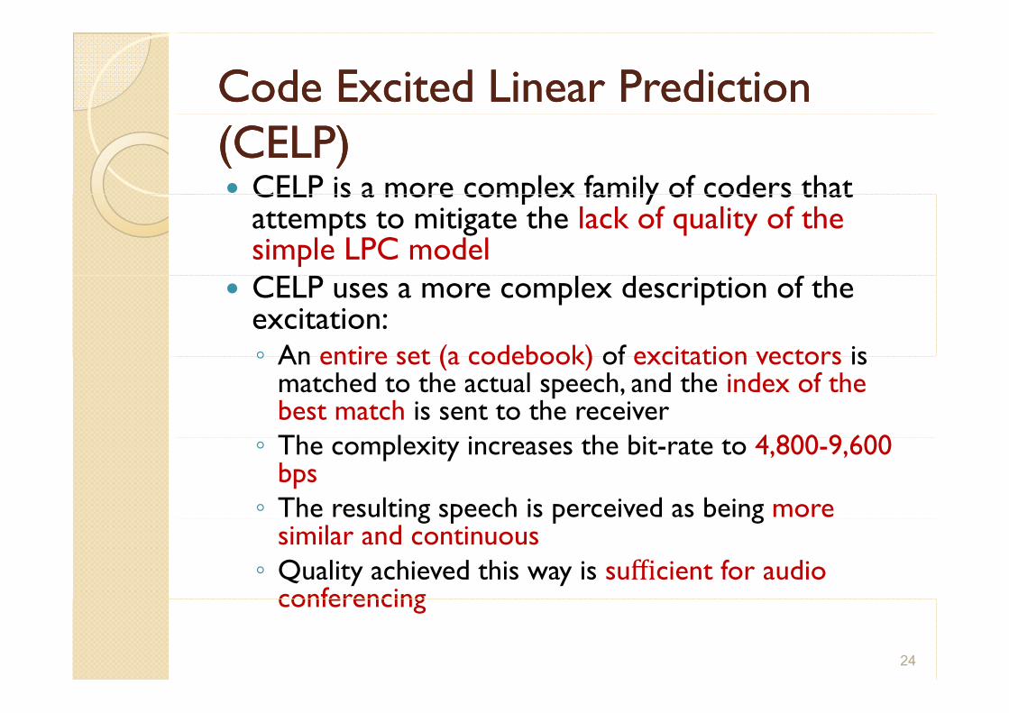
CELP is a more complex family of coders that CELP is a more complex family of coders that attempts to mitigate the lack of quality of the simple LPC model CELP l d f h CELP uses a more complex description of the excitation: ◦ An entire set (a codebook) of excitation vectors is ◦ An entire set (a codebook) of excitation vectors is

matched to the actual speech, and the index of the best match is sent to the receiver Th l i i h bi 4 800 9 600 ◦ The complexity increases the bit-rate to 4,800-9,600 bps ◦ The resulting speech is perceived as being more g p p g

similar and continuous ◦ Quality achieved this way is sufficient for audio

conferencing conferencing

24

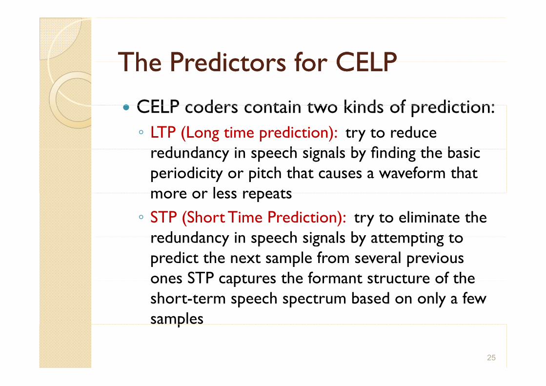
The Predictors for CELP The Predictors for CELP The Predictors for CELP The Predictors for CELP CELP coders contain two kinds of prediction: CELP coders contain two kinds of prediction: ◦ LTP (Long time prediction): try to reduce

d d i h i l b fi di th b i redundancy in speech signals by finding the basic periodicity or pitch that causes a waveform that more or less repeats more or less repeats ◦ STP (Short Time Prediction): try to eliminate the

redundancy in speech signals by attempting to redundancy in speech signals by attempting to predict the next sample from several previous ones STP captures the formant structure of the ones STP captures the formant structure of the short-term speech spectrum based on only a few samples p

25

Relationship between STP and LTP Relationship between STP and LTP Relationship between STP and LTP Relationship between STP and LTP

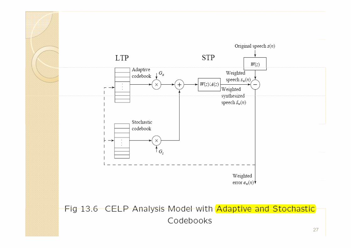
STP captures the formant structure of the STP captures the formant structure of the short-term speech spectrum based on only a few samplespLTP, following STP, recovers the long-term correlation in the speech signal that

h d h represents the periodicity in speech using whole frames or subframes (1/4 of a frame)

LTP i ft i l t d " d ti – LTP is often implemented as "adaptive codebook searching"Fig 13 6 shows the relationship between STP Fig. 13.6 shows the relationship between STP and LTP

26

Adaptive Codebook Searching Adaptive Codebook Searching Adaptive Codebook Searching Adaptive Codebook Searching

Rationale: Rationale: ◦ Look in a codebook of waveforms to find one

that matches the current subframe ◦ Codeword: a shifted speech residue segment

indexed by the by the lag τ corresponding to the current speech frame or subframe in the adaptive codebook ◦ The gain corresponding to the codeword is g p g

denoted as g0

28

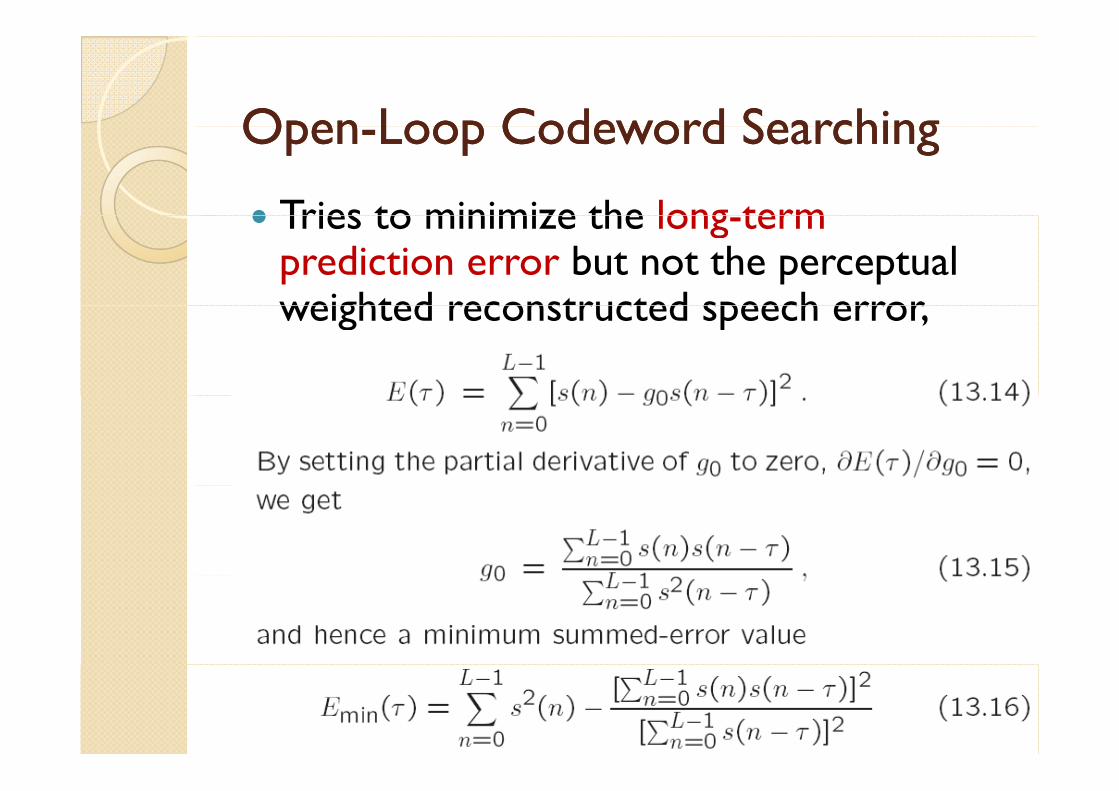
OpenOpen Loop Codeword Searching Loop Codeword Searching OpenOpen--Loop Codeword Searching Loop Codeword Searching

Tries to minimize the long term Tries to minimize the long-term prediction error but not the perceptual weighted reconstructed speech error weighted reconstructed speech error,

29

LZW CloseLZW Close--Loop Codeword Loop Codeword Searching Searching

Closed-loop search is more often used in CELP Closed-loop search is more often used in CELP coders — also called Analysis-By-Synthesis (A-B-S) speech is reconstructed and perceptual error for speech is reconstructed and perceptual error for that is minimized via an adaptive codebook search, rather than simply considering sum-of-squares The best candidate in the adaptive codebook is selected to minimize the distortion of locally reconstructed speech Parameters are found by minimizing a measure of h di b h i i l d h the di erence between the original and the

reconstructed speech

30

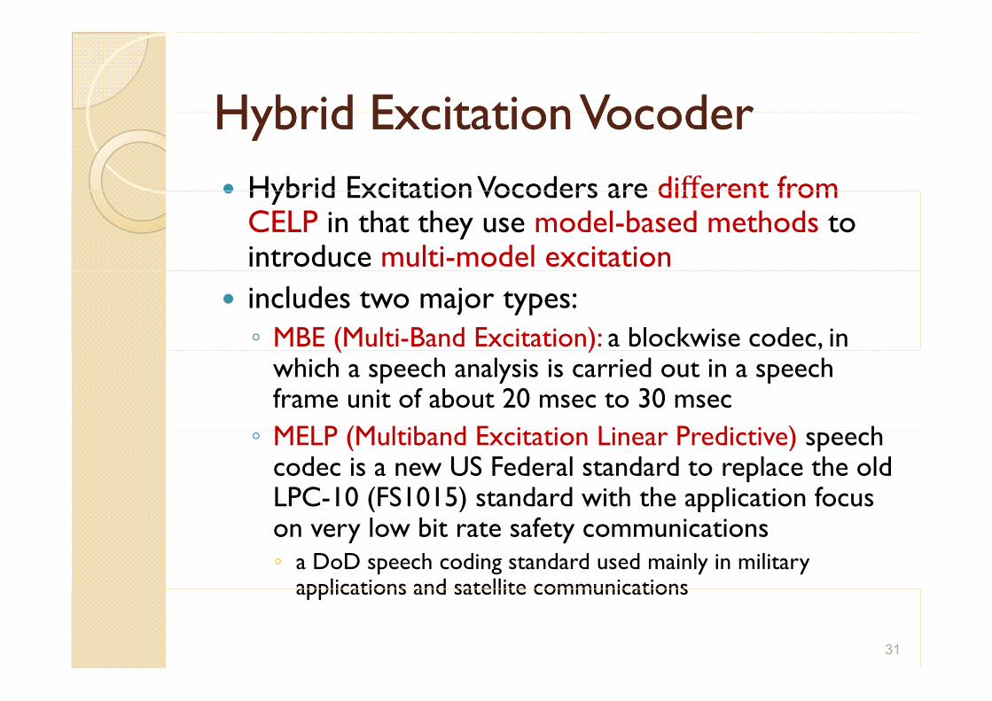
Hybrid Excitation Vocoder Hybrid Excitation Vocoder Hybrid Excitation Vocoder Hybrid Excitation Vocoder Hybrid Excitation Vocoders are di erent from Hybrid Excitation Vocoders are di erent from CELP in that they use model-based methods to introduce multi-model excitation includes two major types: ◦ MBE (Multi-Band Excitation): a blockwise codec, in ( )

which a speech analysis is carried out in a speech frame unit of about 20 msec to 30 msecMELP (M ltib d E it ti Li P di ti ) h ◦ MELP (Multiband Excitation Linear Predictive) speech codec is a new US Federal standard to replace the old LPC-10 (FS1015) standard with the application focus ( ) ppon very low bit rate safety communications ◦ a DoD speech coding standard used mainly in military

applications and satellite communicationsapplications and satellite communications

31

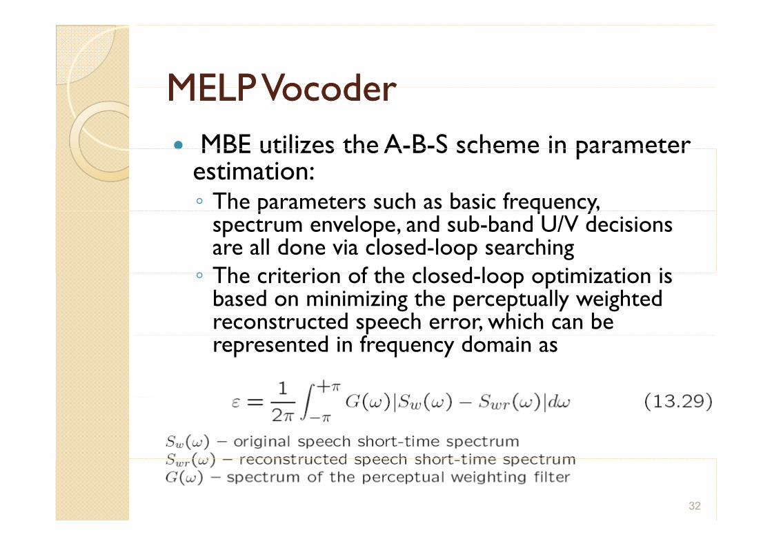
MELP Vocoder MELP Vocoder MELP Vocoder MELP Vocoder MBE utilizes the A-B-S scheme in parameter MBE utilizes the A B S scheme in parameter

estimation: ◦ The parameters such as basic frequency, p q y,

spectrum envelope, and sub-band U/V decisions are all done via closed-loop searching ◦ The criterion of the closed loop optimization is ◦ The criterion of the closed-loop optimization is

based on minimizing the perceptually weighted reconstructed speech error, which can be represented in frequency domain as

32

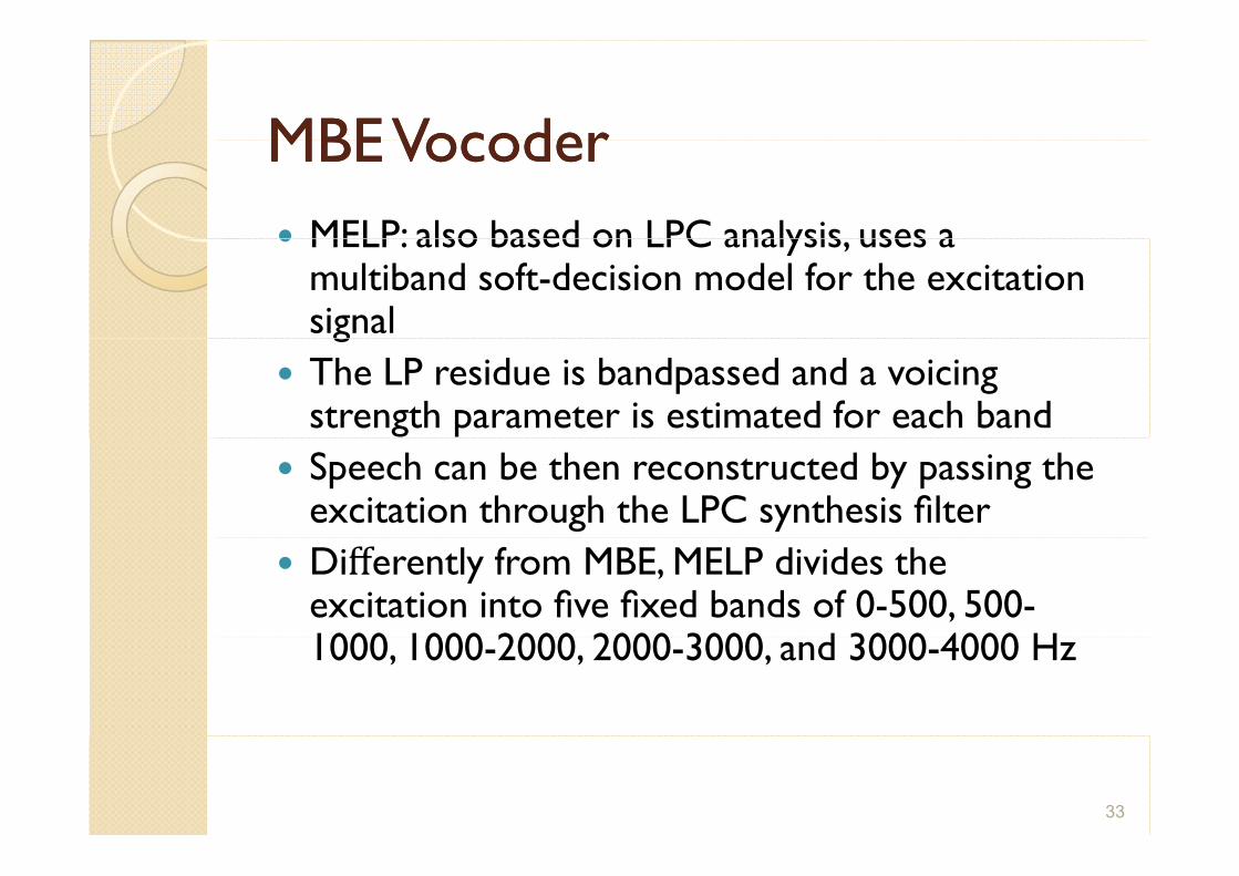
MBE Vocoder MBE Vocoder MBE Vocoder MBE Vocoder MELP: also based on LPC analysis uses a MELP: also based on LPC analysis, uses a multiband soft-decision model for the excitation signal gThe LP residue is bandpassed and a voicing strength parameter is estimated for each band Speech can be then reconstructed by passing the excitation through the LPC synthesis filterDi erently from MBE, MELP divides the excitation into five fixed bands of 0-500, 500-1000 1000 2000 2000 3000 d 3000 4000 H 1000, 1000-2000, 2000-3000, and 3000-4000 Hz

33

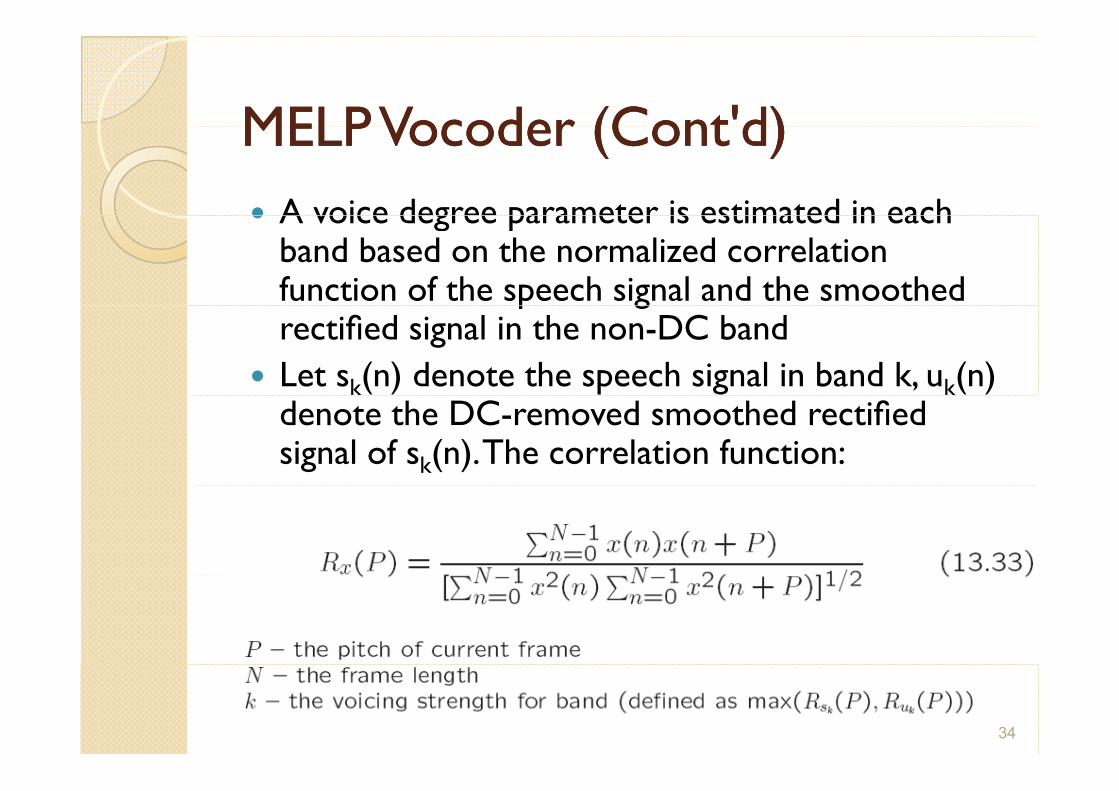
MELP MELP VocoderVocoder (Cont'd) (Cont'd) MELP MELP VocoderVocoder (Cont d) (Cont d) A voice degree parameter is estimated in each A voice degree parameter is estimated in each band based on the normalized correlation function of the speech signal and the smoothed p grectified signal in the non-DC band Let sk(n) denote the speech signal in band k, uk(n) denote the DC-removed smoothed rectifiedsignal of sk(n). The correlation function:

34

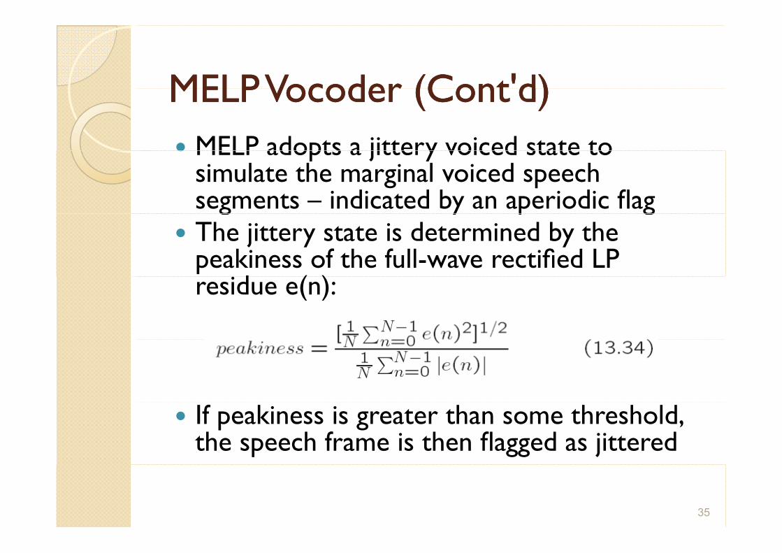
MELP Vocoder (Cont'd) MELP Vocoder (Cont'd) MELP Vocoder (Cont d) MELP Vocoder (Cont d) MELP adopts a jittery voiced state to MELP adopts a jittery voiced state to simulate the marginal voiced speech segments – indicated by an aperiodic flag g y p gThe jittery state is determined by the peakiness of the full-wave rectified LP

d ( ) residue e(n):

If peakiness is greater than some threshold, the speech frame is then flagged as jittered

35

13 4 Further Exploration 13 4 Further Exploration 13.4 Further Exploration 13.4 Further Exploration → Link to Further Exploration for Chapter 13. Link to Further Exploration for Chapter 13.

A comprehensive introduction to speech coding may f S ' be found in Spanias's excellent article in the textbook

references. Sun Microsystems Inc has made available the code Sun Microsystems, Inc. has made available the code for its implementation on standards G.711, G.721, and G.723, in C. The code can be found from the link in the Chapter 13 file in the Further Exploration in the Chapter 13 file in the Further Exploration section of the text website The ITU sells standards; it is linked to from the text website for this Chapter More information on speech coding may be found in the speech FAQ files given as links on the website; the speech FAQ files, given as links on the website; also, links to where LPC and CELP code may be found are included 36

chapter 13 basic audio compression techniques…brahms.emu.edu.tr/babagil/10-comp306-basic audio...

Documents