chapter 11 the stochastic growth model and aggregate ... · chapter 11 the stochastic growth model...

George Alogoskoufis, Dynamic Macroeconomics, 2016

Chapter 11 The Stochastic Growth Model and Aggregate Fluctuations

In previous chapters we studied the long run evolution of output and consumption, real interest rates and real wages, and the long run evolution of the price level and inflation. In order to focus on long-term trends we made the assumption that all markets are competitive and in continuous equilibrium, through the full adjustment of prices, wages and interest rates.

However, as we noted in Chapter 1, economies are characterized by fluctuations in relation to their long-term trends. In some periods output, consumption and employment grow at high rates, while at other times they grow at low or even negative rates. In some periods unemployment is low and in others quite high. Inflation displays significant fluctuations as well.

Understanding the determinants of aggregate fluctuations is the second main objective of macroeconomics. In this, and the chapters that follow, we present the main theories regarding the nature of aggregate fluctuations.

In this chapter we start by introducing competitive equilibrium models of aggregate fluctuations. These are dynamic stochastic general equilibrium models (DSGE), based on optimizing households and firms, flexible wages and prices, and fully competitive markets. Fluctuations in these models are caused by real shocks, mainly exogenous shocks to productivity. The effects of these shocks are propagated through endogenous dynamic processes, such as consumption and investment.

We start with the so called stochastic growth model, which is an extended stochastic version of the Ramsey model. The utility function of a representative household depends on both consumption of goods and services and leisure, while random disturbances to real factors, such as productivity, cause aggregate fluctuations. 1

To be able to arrive at a tractable model, we make simplifying assumptions regarding production and utility functions. Without them these model become extremely complicated. The dynamic analysis is conducted in discrete rather than continuous time.

As the main impulses that generate aggregate fluctuations in the stochastic growth model are real, this model belongs to a class of models that is often referred to as real business cycle models (RBC). Monetary shocks have no real effects on output, employment and capital accumulation in

The original stochastic growth model was presented by Brock and Mirman (1971), and was essentially a Ramsey 1

model, augmented by stochastic shocks to productivity. Later models allowed for variable labor supply, encompassing the intertemporal substitution hypothesis of Lucas and Rapping (1969). The approach analyzed in this chapter follows Kydland and Prescott (1982), Long and Plosser (1983) and Prescott (1986). It is surveyed in King and Rebelo (1999). As we shall see, this approach has also influenced the “new keynesian” approach to aggregate fluctuations, which now also relies on dynamic stochastic general equilibrium models (DSGE).

George Alogoskoufis, Dynamic Macroeconomics, 2016 Chapter 11

this class of models, and only affect real money balances, and nominal variables such as the price level, inflation and nominal wages and interest rates.

11.1 The Stochastic Growth Model

As we have seen in Chapter 1, aggregate fluctuations are not characterized by deterministic cyclical regularities but seem to be characterized by randomness. The prevailing view, which dates back to Frisch (1930) and Slutsky (1937), is that economies are subject to various kinds of random disturbances, which, through the operation of economic transmission mechanisms, affect output, employment, real wages, real interest rates, the price level and inflation, and set in motion dynamic stochastic adjustment processes.

The first model we shall focus on is the so-called stochastic growth model. This is a competitive dynamic stochastic general equilibrium model, without externalities, asymmetric information, frictions and other imperfections of markets.

This model is essentially a generalization of the Ramsey model. It not only excludes any market imperfections, but also all issues related to the heterogeneity of economic agents. The extended Ramsey model is therefore seen as the natural starting point for the study of aggregate fluctuations, in the same way that the original Ramsey model is seen as the “natural” starting point for the study of long run growth.

There are two directions in which the Ramsey must be extended in order to study aggregate fluctuations.

First, one should allow for random disturbances, which can cause fluctuations. As we have seen, without random disturbances, the Ramsey model converges to a unique steady state. The disturbances usually introduced in the Ramsey model are disturbances in total factor productivity (technology shocks), as well as real demand shocks, such as shocks to the preferences of consumers or real government expenditure. Since both kinds of shocks are real - unlike monetary or nominal shocks - this model turns out to be a real business cycle model (RBC). 2

Second, in order to explain fluctuations not only in total output, but also employment, employment must become endogenous in the Ramsey model. This is achieved through the introduction of employment in the utility function of a representative household, in order to allow for endogenous labor supply.

11.1.1 Extending the Ramsey Model to Account for Aggregate Fluctuations

The extended Ramsey model which we end up with is a dynamic stochastic general equilibrium model (DSGE), in which fluctuations are caused by real shocks.

There are a number of identical households and firms, so this is a competitive representative household model. Firms use labor and capital in order produce a homogeneous product. They choose investment and employment in order to maximize their profits, while households choose consumption and labor supply in order to maximize their intertemporal utility.

The extension of the Ramsey model to allow for stochastic shocks to productivity was first attempted by Brock and 2

Mirman (1971), who were the first analyze the stochastic growth model, assuming an exogenous labor supply.!2


The key variables and parameters of the model are as follows:

Y total output K physical capital L employment A labor efficiency (productivity) C total private consumption CG total real government expenditure N total population δ depreciation rate of capital ρ pure rate of time preference of households r real interest rate W real wage per employee

11.1.2 The Behavior of Firms

The economy consists of a large number of identical households and firms, interacting through competitive markets. Output and factor prices are thus given for every household and every firm.

The representative firm has a production function with constant returns to scale, which takes the Cobb-Douglas form. Thus, the aggregate production function is also Cobb Douglas.

! 0<α<1 (11.1)

The demand for output consists of private consumption, investment and government consumption. Government consumption is financed through non distortionary taxation, and, in each period, taxes are equal to government consumption. Thus, the equilibrium condition in the output market is given by,

! (11.2)

Solving (11.2) for K$ we get a capital accumulation equation of the form,

! (11.3)

To the extent that total savings Y-C-CG exceed depreciation investment δΚ, there is accumulation of capital.

Labor and capital are paid their marginal product, as firms maximize profits taking the real interest rate r and the real wage W as given.

! (11.4)

Yt = Kα (AtLt )

1−α

Yt = Ct +CtG + Kt+1 − Kt +δKt

t+1

Kt+1 = Kt +Yt −Ct −CtG −δKt

Wt = (1−α )Kt

AtLt

⎛⎝⎜

⎞⎠⎟

α

At

!3


$ (11.5)

(11.1)-(11.5) describe the behavior of firms. Firms are assumed to employ workers up to the point where the marginal product of labor is equal to the real wage, and capital up to the point where the marginal product of capital equals the real user cost of capital, assumed to be equal to the real interest rate plus the depreciation rate.

11.1.3 The Representative Household

The economy is inhabited by a large number of identical households, each of which has an infinite time horizon. The representative household maximizes its expected intertemporal utility function, which depends on the path of real consumption of goods and services and leisure. The utility function is defined by,

! (11.6)

where E is the mathematical expectations operator and u is the per capita instantaneous utility of the representative household. Per capita consumption is given by c=C/N and per capita employment by l=L/N. We shall assume that the instantaneous utility function is log-linear.

! , b > 0 (11.7)

This assumption is made in order to arrive at simpler functional relationships. However, like all simplifications, this assumption implies specific properties for the model.

11.1.4 Population, Efficiency of Labor and Government Expenditure

Population increases exogenously at a rate n per period. Consequently,

! , n < ρ (11.8)

The final assumptions of the model concern the behavior of the two main exogenous variables. Both productivity (labor efficiency), and government expenditure are supposed to be subject to random disturbances.

The stochastic process describing the evolution of the efficiency of labor is given by, 3

! (11.9)

where,

rt =αAtLtKt

⎛⎝⎜

⎞⎠⎟

1−α

−δ

U = Et1

1+ ρ⎛⎝⎜

⎞⎠⎟

t+s

u(ct+s ,1− lt+s )Nt+s

Hs=0

∞∑

ut = lnct + b ln(1− lt )

lnNt = n_+ nt

lnAt = a_+ gt + at

Mathematical Annex 4 contains an introduction to stochastic processes.3

!4


! -1<η$ <1 (11.10)

εA follows a white noise stochastic process.

(11.9) and (11.10) imply that labor efficiency grows at an exogenous rate g, but that it is subject to random disturbances a that follow a stationary first order autoregressive process. The assumptions about (11.10) imply that the impact of a technological disturbance is gradually reduced over time.

Similar assumptions are made regarding the stochastic process that describes the evolution of real government expenditure. We assume that real government expenditure is growing at an average rate n+g, i.e. that on average it remains constant relative to total output. However, we also assume that real government expenditure is subject to disturbances follow a stationary first order autoregressive process. More particularly,

! (11.11)

where,

! -1<η$ <1 (11.12)

εG follows a white noise stochastic process. 4

These elements complete the structure of the model. The two most important differences from the original Ramsey model are, first, the introduction of leisure time in the utility function of the representative household, which potentially allows for fluctuations in employment, and, second, the introduction of random disturbances to labor efficiency (productivity) and government expenditure, which lead to fluctuations around a long-term trend.

Before we look at the general properties of the model, it is worth considering the implications for the behavior of the representative household of the introduction of leisure in the utility function, as well as the implications of uncertainty, in the form of random disturbances.

11.1.5 Labor Supply of the Representative Household

The first difference of this model from the Ramsey model arises from the introduction of leisure time in the utility function of the household, which makes labor supply endogenous. To analyze the importance of this addition, let us first consider the problem of a household that lives for a single time period and has no assets. The problem of that household is defined as the maximization of,

!

under the constraint c = Wl.

The Lagrangian is defined by,

at =ηAat−1 + ε tA

A

lnGt = cg_

+ (n + g)t + ctG

ctG =ηGct−1

G + ε tG

G

lnc + b ln(1− l)

The assumption that the processes driving labor productivity and real government expenditure are AR(1) are made for 4

simplicity, and can of course be generalized.!5


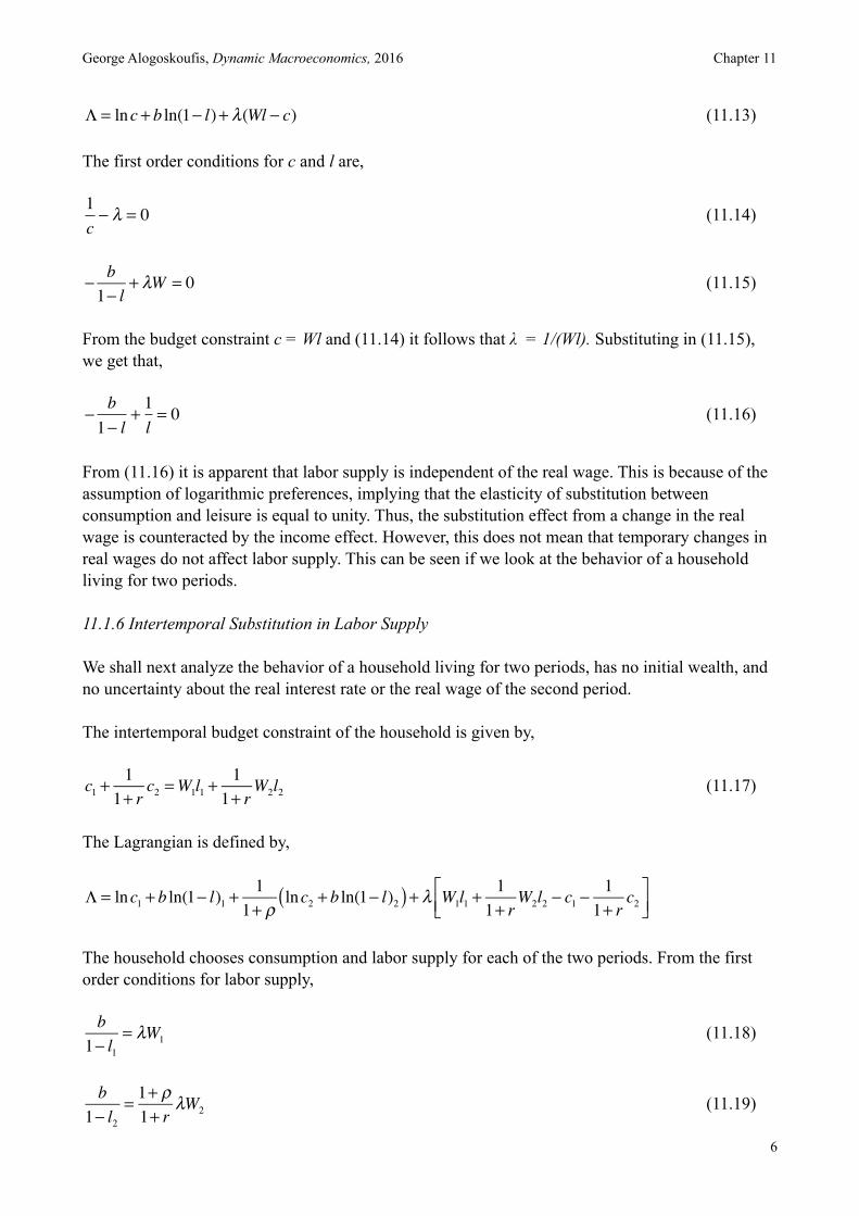
! (11.13)

The first order conditions for c and l are,

! (11.14)

! (11.15)

From the budget constraint c = Wl and (11.14) it follows that λ = 1/(Wl). Substituting in (11.15), we get that,

! (11.16)

From (11.16) it is apparent that labor supply is independent of the real wage. This is because of the assumption of logarithmic preferences, implying that the elasticity of substitution between consumption and leisure is equal to unity. Thus, the substitution effect from a change in the real wage is counteracted by the income effect. However, this does not mean that temporary changes in real wages do not affect labor supply. This can be seen if we look at the behavior of a household living for two periods.

11.1.6 Intertemporal Substitution in Labor Supply

We shall next analyze the behavior of a household living for two periods, has no initial wealth, and no uncertainty about the real interest rate or the real wage of the second period.

The intertemporal budget constraint of the household is given by,

! (11.17)

The Lagrangian is defined by,

!

The household chooses consumption and labor supply for each of the two periods. From the first order conditions for labor supply,

! (11.18)

! (11.19)

Λ = lnc + b ln(1− l)+ λ(Wl − c)

1c− λ = 0

− b1− l

+ λW = 0

−b1− l

+1l= 0

c1 +11+ r

c2 =W1l1 +11+ r

W2l2

Λ = lnc1 + b ln(1− l)1 +1

1+ ρlnc2 + b ln(1− l)2( )+ λ W1l1 +

11+ r

W2l2 − c1 −11+ r

c2⎡⎣⎢

⎤⎦⎥

b1− l1

= λW1

b1− l2

= 1+ ρ1+ r

λW2

!6


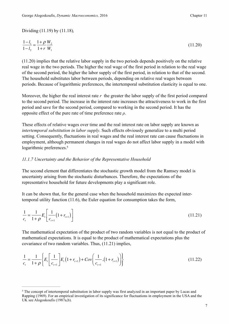
Dividing (11.19) by (11.18),

! (11.20)

(11.20) implies that the relative labor supply in the two periods depends positively on the relative real wage in the two periods. The higher the real wage of the first period in relation to the real wage of the second period, the higher the labor supply of the first period, in relation to that of the second. The household substitutes labor between periods, depending on relative real wages between periods. Because of logarithmic preferences, the intertemporal substitution elasticity is equal to one.

Moreover, the higher the real interest rate r the greater the labor supply of the first period compared to the second period. The increase in the interest rate increases the attractiveness to work in the first period and save for the second period, compared to working in the second period. It has the opposite effect of the pure rate of time preference rate ρ.

These effects of relative wages over time and the real interest rate on labor supply are known as intertemporal substitution in labor supply. Such effects obviously generalize to a multi period setting. Consequently, fluctuations in real wages and the real interest rate can cause fluctuations in employment, although permanent changes in real wages do not affect labor supply in a model with logarithmic preferences. 5

11.1.7 Uncertainty and the Behavior of the Representative Household

The second element that differentiates the stochastic growth model from the Ramsey model is uncertainty arising from the stochastic disturbances. Therefore, the expectations of the representative household for future developments play a significant role.

It can be shown that, for the general case when the household maximizes the expected intertemporal utility function (11.6), the Euler equation for consumption takes the form,

! (11.21)

The mathematical expectation of the product of two random variables is not equal to the product of mathematical expectations. It is equal to the product of mathematical expectations plus the covariance of two random variables. Thus, (11.21) implies,

! (11.22)

1− l11− l2

= 1+ ρ1+ r

W2

W1

1ct

=1

1+ ρEt

1ct+1

1+ rt+1( )⎡

⎣⎢

⎤

⎦⎥

1ct

=1

1+ ρEt

1ct+1

⎡

⎣⎢

⎤

⎦⎥

⎧⎨⎪

⎩⎪Et 1+ rt+1( ) + Cov 1

ct+1, 1+ rt+1( )⎛

⎝⎜⎞⎠⎟⎫⎬⎪

⎭⎪

The concept of intertemporal substitution in labor supply was first analyzed in an important paper by Lucas and 5

Rapping (1969). For an empirical investigation of its significance for fluctuations in employment in the USA and the UK see Alogoskoufis (1987a,b).

!7


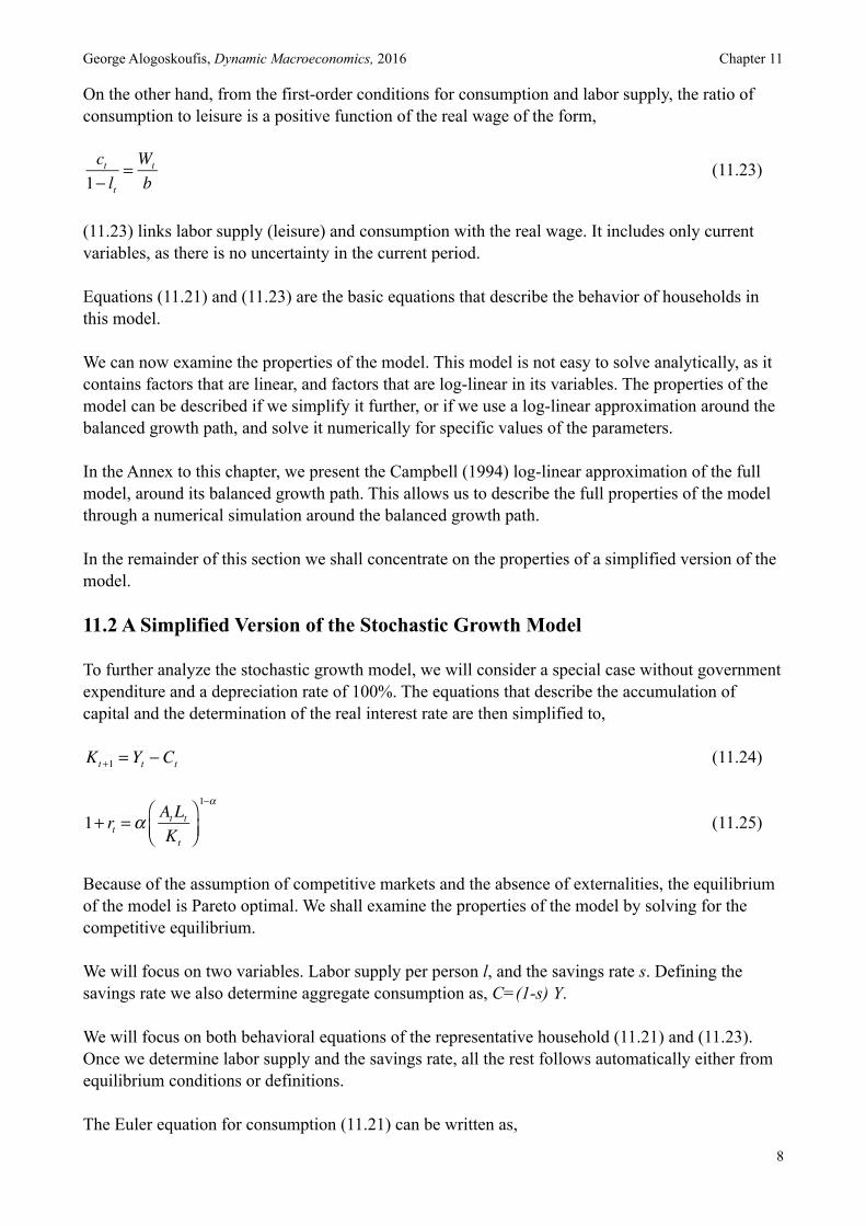
On the other hand, from the first-order conditions for consumption and labor supply, the ratio of consumption to leisure is a positive function of the real wage of the form,

! (11.23)

(11.23) links labor supply (leisure) and consumption with the real wage. It includes only current variables, as there is no uncertainty in the current period.

Equations (11.21) and (11.23) are the basic equations that describe the behavior of households in this model.

We can now examine the properties of the model. This model is not easy to solve analytically, as it contains factors that are linear, and factors that are log-linear in its variables. The properties of the model can be described if we simplify it further, or if we use a log-linear approximation around the balanced growth path, and solve it numerically for specific values of the parameters.

In the Annex to this chapter, we present the Campbell (1994) log-linear approximation of the full model, around its balanced growth path. This allows us to describe the full properties of the model through a numerical simulation around the balanced growth path.

In the remainder of this section we shall concentrate on the properties of a simplified version of the model.

11.2 A Simplified Version of the Stochastic Growth Model

To further analyze the stochastic growth model, we will consider a special case without government expenditure and a depreciation rate of 100%. The equations that describe the accumulation of capital and the determination of the real interest rate are then simplified to,

! (11.24)

! (11.25)

Because of the assumption of competitive markets and the absence of externalities, the equilibrium of the model is Pareto optimal. We shall examine the properties of the model by solving for the competitive equilibrium.

We will focus on two variables. Labor supply per person l, and the savings rate s. Defining the savings rate we also determine aggregate consumption as, C=(1-s) Y.

We will focus on both behavioral equations of the representative household (11.21) and (11.23). Once we determine labor supply and the savings rate, all the rest follows automatically either from equilibrium conditions or definitions.

The Euler equation for consumption (11.21) can be written as,

ct1− lt

= Wt

b

Kt+1 = Yt − Ct

1+ rt =αAtLtKt

⎛⎝⎜

⎞⎠⎟

1−α

!8


!

After we use the relations that,

! , ! , !

we get that,

!

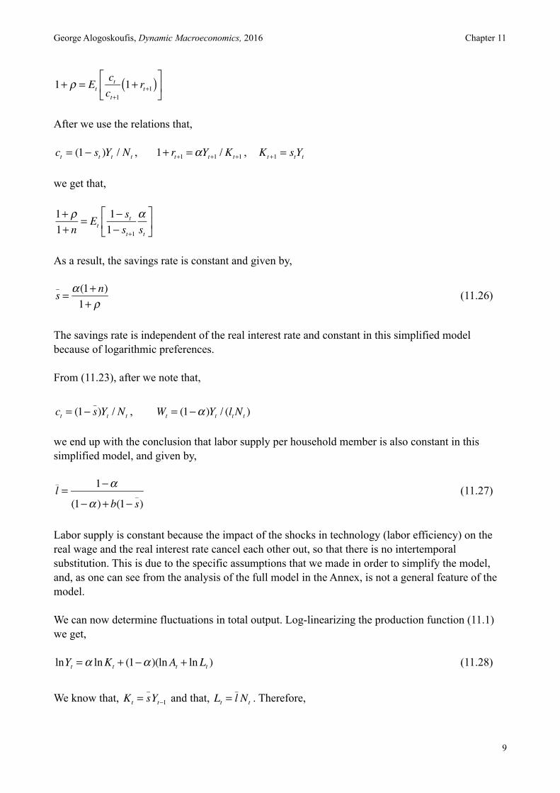
As a result, the savings rate is constant and given by,

! (11.26)

The savings rate is independent of the real interest rate and constant in this simplified model because of logarithmic preferences.

From (11.23), after we note that,

! , !

we end up with the conclusion that labor supply per household member is also constant in this simplified model, and given by,

! (11.27)

Labor supply is constant because the impact of the shocks in technology (labor efficiency) on the real wage and the real interest rate cancel each other out, so that there is no intertemporal substitution. This is due to the specific assumptions that we made in order to simplify the model, and, as one can see from the analysis of the full model in the Annex, is not a general feature of the model.

We can now determine fluctuations in total output. Log-linearizing the production function (11.1) we get,

! (11.28)

We know that, ! and that, ! . Therefore,

1+ ρ = Etctct+1

1+ rt+1( )⎡

⎣⎢

⎤

⎦⎥

ct = (1− st )Yt / Nt 1+ rt+1 =αYt+1 /Kt+1 Kt+1 = stYt

1+ ρ1+ n

= Et1− st1− st+1

αst

⎡

⎣⎢

⎤

⎦⎥

s_= α (1+ n)1+ ρ

ct = (1− s_)Yt / Nt Wt = (1−α )Yt / (ltNt )

l_= 1−α

(1−α )+ b(1− s_)

lnYt =α lnKt + (1−α )(lnAt + lnLt )

Kt = s_Yt−1 Lt = l

_Nt

!9


! (11.29)

We can substitute the logarithm of A and N from equations (11.8) and (11.9). This implies,

! (11.30)

We can express (11.30), as,

! (11.31)

where,

! , are percentage deviations of output from trend output.

The logarithm of trend output, is defined as,

!

From (11.10) and (11.31), we end up with,

! (11.32)

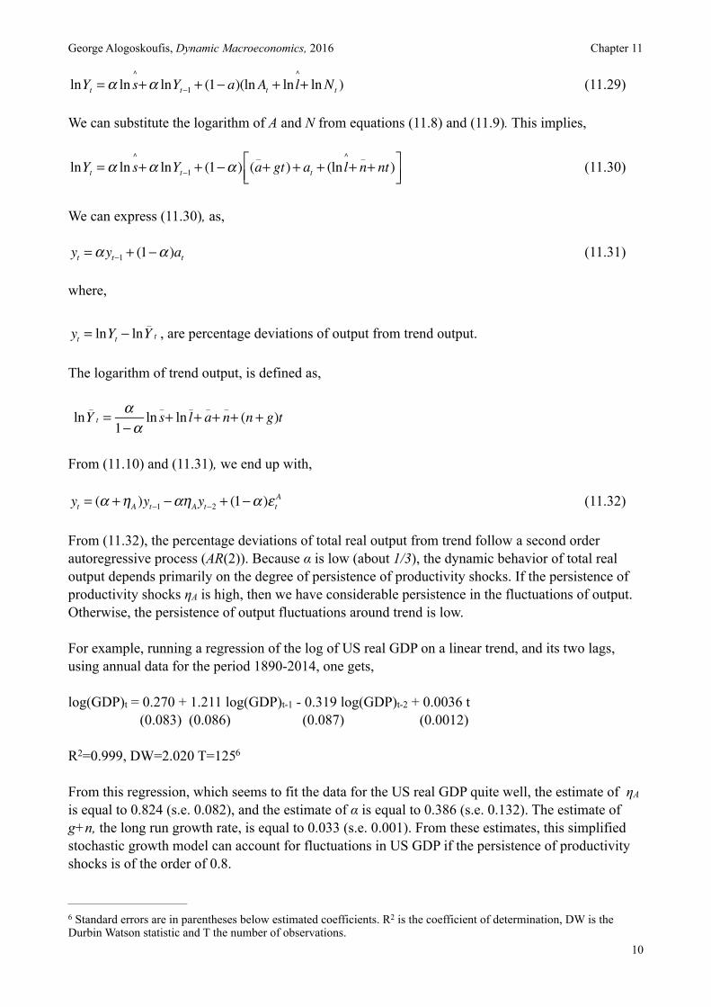
From (11.32), the percentage deviations of total real output from trend follow a second order autoregressive process (AR(2)). Because α is low (about 1/3), the dynamic behavior of total real output depends primarily on the degree of persistence of productivity shocks. If the persistence of productivity shocks ηA is high, then we have considerable persistence in the fluctuations of output. Otherwise, the persistence of output fluctuations around trend is low.

For example, running a regression of the log of US real GDP on a linear trend, and its two lags, using annual data for the period 1890-2014, one gets,

log(GDP)t = 0.270 + 1.211 log(GDP)t-1 - 0.319 log(GDP)t-2 + 0.0036 t (0.083) (0.086) (0.087) (0.0012)

R2=0.999, DW=2.020 T=125 6

From this regression, which seems to fit the data for the US real GDP quite well, the estimate of ηA is equal to 0.824 (s.e. 0.082), and the estimate of α is equal to 0.386 (s.e. 0.132). The estimate of g+n, the long run growth rate, is equal to 0.033 (s.e. 0.001). From these estimates, this simplified stochastic growth model can account for fluctuations in US GDP if the persistence of productivity shocks is of the order of 0.8.

lnYt =α ln s^+α lnYt−1 + (1− a)(lnAt + ln l

^+ lnNt )

lnYt =α ln s^+α lnYt−1 + (1−α ) (a

_+ gt)+ at + (ln l

^+ n

_+ nt)⎡

⎣⎢⎤⎦⎥

yt =α yt−1 + (1−α )at

yt = lnYt − lnY_t

lnY_t =

α1−α

ln s_+ ln l

_+ a

_+ n

_+ (n + g)t

yt = (α +ηA )yt−1 −αηAyt−2 + (1−α )ε tA

Standard errors are in parentheses below estimated coefficients. R2 is the coefficient of determination, DW is the 6

Durbin Watson statistic and T the number of observations.!10


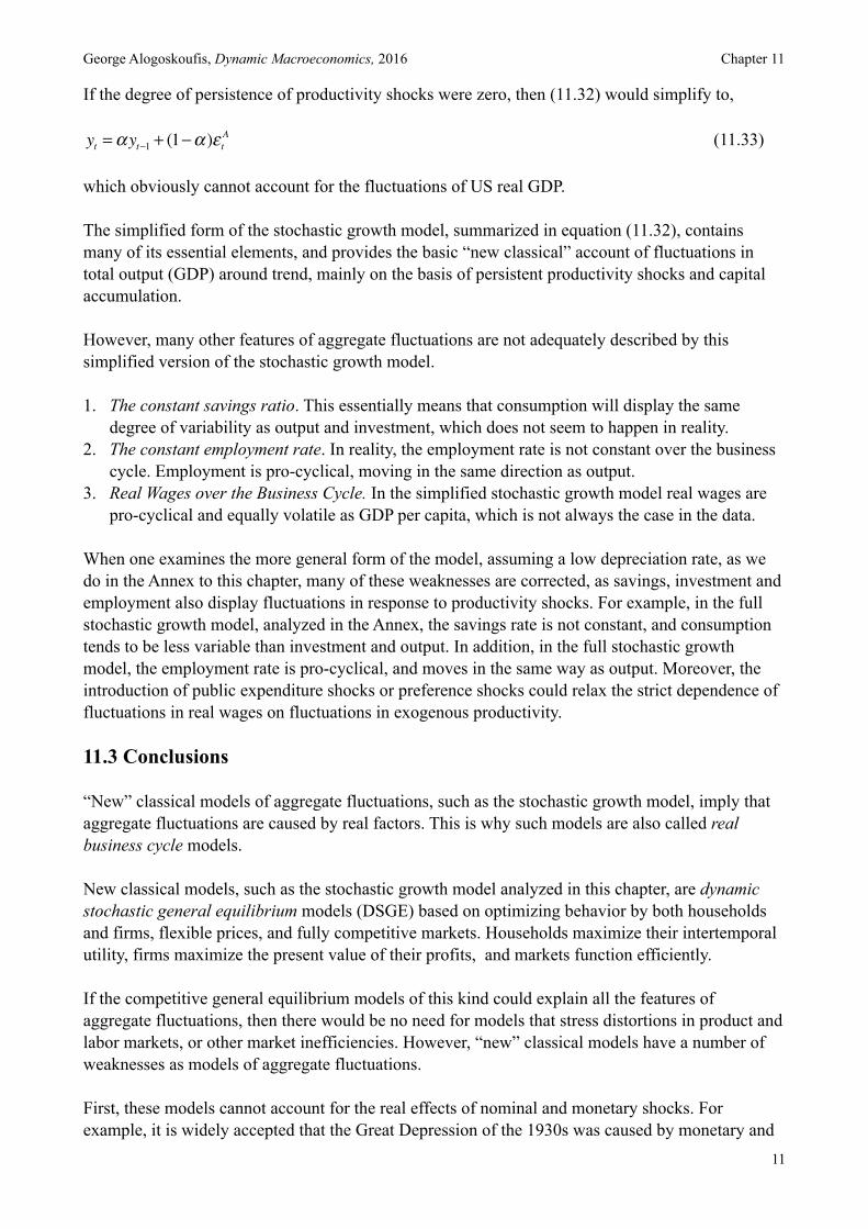
If the degree of persistence of productivity shocks were zero, then (11.32) would simplify to,

! (11.33)

which obviously cannot account for the fluctuations of US real GDP.

The simplified form of the stochastic growth model, summarized in equation (11.32), contains many of its essential elements, and provides the basic “new classical” account of fluctuations in total output (GDP) around trend, mainly on the basis of persistent productivity shocks and capital accumulation.

However, many other features of aggregate fluctuations are not adequately described by this simplified version of the stochastic growth model.

1. The constant savings ratio. This essentially means that consumption will display the same degree of variability as output and investment, which does not seem to happen in reality.

2. The constant employment rate. In reality, the employment rate is not constant over the business cycle. Employment is pro-cyclical, moving in the same direction as output.

3. Real Wages over the Business Cycle. In the simplified stochastic growth model real wages are pro-cyclical and equally volatile as GDP per capita, which is not always the case in the data.

When one examines the more general form of the model, assuming a low depreciation rate, as we do in the Annex to this chapter, many of these weaknesses are corrected, as savings, investment and employment also display fluctuations in response to productivity shocks. For example, in the full stochastic growth model, analyzed in the Annex, the savings rate is not constant, and consumption tends to be less variable than investment and output. In addition, in the full stochastic growth model, the employment rate is pro-cyclical, and moves in the same way as output. Moreover, the introduction of public expenditure shocks or preference shocks could relax the strict dependence of fluctuations in real wages on fluctuations in exogenous productivity.

11.3 Conclusions

“New” classical models of aggregate fluctuations, such as the stochastic growth model, imply that aggregate fluctuations are caused by real factors. This is why such models are also called real business cycle models.

New classical models, such as the stochastic growth model analyzed in this chapter, are dynamic stochastic general equilibrium models (DSGE) based on optimizing behavior by both households and firms, flexible prices, and fully competitive markets. Households maximize their intertemporal utility, firms maximize the present value of their profits, and markets function efficiently.

If the competitive general equilibrium models of this kind could explain all the features of aggregate fluctuations, then there would be no need for models that stress distortions in product and labor markets, or other market inefficiencies. However, “new” classical models have a number of weaknesses as models of aggregate fluctuations.

First, these models cannot account for the real effects of nominal and monetary shocks. For example, it is widely accepted that the Great Depression of the 1930s was caused by monetary and

yt =α yt−1 + (1−α )ε tA

!11


not real shocks. Similar views are prevalent regarding the causes of the recession of 2008-09, which was one of the deepest post World War II recessions. The imperfect information assumption of Lucas (1972, 1973) can be used for accounting for the real effects of nominal shocks in this model, but the effects of nominal shocks would be short lived and not particularly persistent.

Second, even though “new”classical models can account for employment fluctuations, they only do so on the basis of intertemporal substitution in labor supply. This explanation, however, is not sufficient to explain the existence and the persistence of unemployment and the widely held view among economists and non-economists, that unemployment is an involuntary condition for those who experience it, and not the result of a voluntary rational choice.

For these reasons, and despite the fact that the stochastic growth model is theoretically consistent, many economists consider it as an extreme explanation of aggregate fluctuations. The alternative class of models are “keynesian” models, which assume that nominal wages and/or prices cannot adjust immediately in order to equilibrate labor and product markets. Thus, following nominal shocks, quantities have to adjust too, resulting in fluctuations in real variables, deviations of output and other real variables from their steady state values and involuntary unemployment. It is to these models that we shall now turn, starting with an examination of the “keynesian” approach in the following chapter.

!12


Annex to Chapter 11: A Log-Linear Approximation to the Stochastic Growth Model

This Annex sets out the full stochastic growth model and derives an approximate analytical solution, based on a log-linear approximation around the steady state equilibrium. Following Campbell (1994), the model is thus transformed into a system of log-linear stochastic difference equations, which can be solved by the method of undetermined coefficients. We shall solve the model assuming that government expenditure is equal to zero.

The first equation of the model is the production function,

! , 0<α<1 (A.11.1)

The second is the capital accumulation process,

! (A.11.2)

Finally there is a representative household which maximizes,

! (A.11.3)

subject to the accumulation process (A.11.2).

Firms maximize profits, subject to the production function, and set the marginal product of capital and labor equal to the real interest rate and the real wage respectively. It thus follows that,

! (A.11.4)

! (A.11.5)

From the first order conditions for the maximization of the utility of the representative household it also follows that,

! (A.11.6)

! (A.11.7)

Yt = Kα (AtLt )

1−α

Kt+1 = (1−δ )Kt +Yt −Ct

U = Et1

1+ ρ⎛⎝⎜

⎞⎠⎟

t

lnCt + b ln(Nt − Lt )( )t=0

∞∑

wt = (1−α )Kt

AtLt

⎛⎝⎜

⎞⎠⎟

α

At

rt =αAtLtKt

⎛⎝⎜

⎞⎠⎟

1−α

−δ

1Ct

= 1+ n1+ ρ

Et1Ct+1

1+ rt+1( )⎡

⎣⎢

⎤

⎦⎥

Ct

Nt − Lt= wt

b

!13


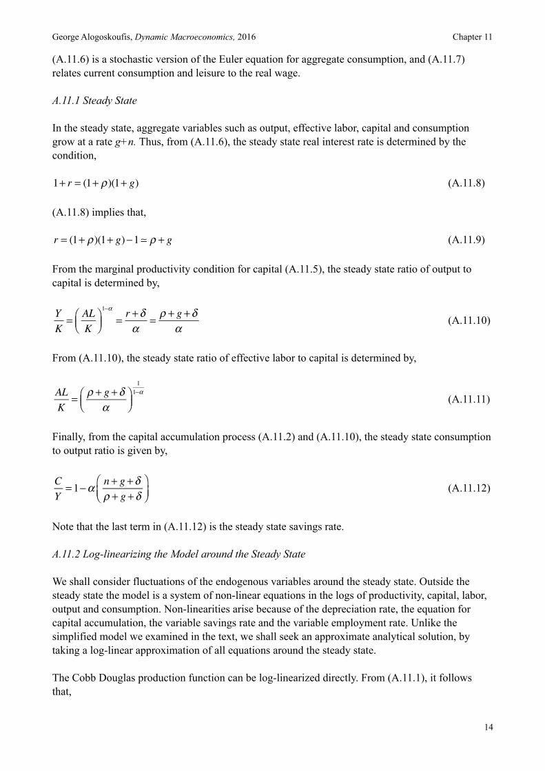
(A.11.6) is a stochastic version of the Euler equation for aggregate consumption, and (A.11.7) relates current consumption and leisure to the real wage.

A.11.1 Steady State

In the steady state, aggregate variables such as output, effective labor, capital and consumption grow at a rate g+n. Thus, from (A.11.6), the steady state real interest rate is determined by the condition,

! (A.11.8)

(A.11.8) implies that,

! (A.11.9)

From the marginal productivity condition for capital (A.11.5), the steady state ratio of output to capital is determined by,

! (A.11.10)

From (A.11.10), the steady state ratio of effective labor to capital is determined by,

! (A.11.11)

Finally, from the capital accumulation process (A.11.2) and (A.11.10), the steady state consumption to output ratio is given by,

! (A.11.12)

Note that the last term in (A.11.12) is the steady state savings rate.

A.11.2 Log-linearizing the Model around the Steady State

We shall consider fluctuations of the endogenous variables around the steady state. Outside the steady state the model is a system of non-linear equations in the logs of productivity, capital, labor, output and consumption. Non-linearities arise because of the depreciation rate, the equation for capital accumulation, the variable savings rate and the variable employment rate. Unlike the simplified model we examined in the text, we shall seek an approximate analytical solution, by taking a log-linear approximation of all equations around the steady state.

The Cobb Douglas production function can be log-linearized directly. From (A.11.1), it follows that,

1+ r = (1+ ρ)(1+ g)

r = (1+ ρ)(1+ g)−1! ρ + g

YK

= ALK

⎛⎝⎜

⎞⎠⎟1−α

= r +δα

= ρ + g +δα

ALK

= ρ + g +δα

⎛⎝⎜

⎞⎠⎟

11−α

CY

= 1−α n + g +δρ + g +δ

⎛⎝⎜

⎞⎠⎟

!14


! (A.11.13)

where lowercase letters denote the difference of the log of the relevant variable from its steady state value.

The capital accumulation equation (A.11.2) is obviously not log-linear. Dividing by Kt , it can be written as,

! (A.11.14)

Taking logs, (A.11.14) can be written as,

! (A.11.15)

Taking a first order Taylor approximation of (A.11.15) around the steady state, and using the log-linear version of the production function (A.11.13), we end up with the following log-linear approximation of the accumulation equation around the steady state,

! (A.11.16)

where,

! , ! .

We next turn to the determination of the real interest rate and the Euler equation for consumption.

From the marginal productivity condition for capital, (A.11.5), it follows that,

! (A.11.17)

Taking a log-linear approximation of (A.11.17) around the steady state, we get that,

! (A.11.18)

where,

! .

Substituting (A.11.18) in the Euler equation for consumption (A.11.6), and assuming the variables on the right hand side are jointly log-normal and homoskedastic, the Euler equation for consumption can be written as,

yt =αkt + (1−α )(at + lt )

Kt+1

Kt

− (1−δ )⎛⎝⎜

⎞⎠⎟= YtKt

1− Ct

Yt

⎛⎝⎜

⎞⎠⎟

ln[eΔkt+1 − (1−δ )]= yt − kt + ln[1− e(ct−yt ) ]

kt+1 ! λ1kt + λ2 (at + lt )+ (1− λ1 − λ2 )ct

λ1 =1+ ρ + g1+ g

λ2 =(1−α )(ρ + g +δ )

α (1+ g)

1+ rt+1 =αAt+1Lt+1Kt+1

⎛⎝⎜

⎞⎠⎟

1−α

+ (1−δ )

rt+1 ! λ3 at+1 + lt+1 − kt+1( )

λ3 =(1−α )(ρ + g +δ )

1+ ρ + g

!15


! (A.11.19)

Log-linearizing the marginal productivity condition for labor (A.11.4), and taking deviations from steady state, we get that deviations of the log of the real wage from steady state are given by,

! (A.11.20)

Finally, log-linearizing the first order condition for consumption and leisure, (A.11.7), using the marginal productivity condition for employment (A.11.20) to substitute for the logarithm of the real wage, we get,

! (A.11.21)

where,

! .

! is the steady state labor supply as a percentage of total available time. Following Prescott (1986) we shall assume that this is equal to one third.

In order to close the model, we need only specify the exogenous stochastic process driving productivity a. We shall continue to assume, as in the main text, that it follows an AR(1) process of the form,

! , ! (A.11.22)

A.11.3 Solving the Model

The model consists of equations (A.11.13), (A.11.16), (A.11.18), (A.11.19), (A.11.20), (A.11.21), and determines fluctuations around the steady state for output, the capital stock, consumption, employment, the real interest and the real wage. The exogenous shock driving the fluctuations is a productivity (technological) shock, that follows the AR(1) process in (A.11.22).

We can first solve the sub-system of (A.11.16), (A.11.19) and (A.11.21) for capital, employment and consumption, and then substitute in the other three equations to determine output, the real interest rate and the real wage.

The easiest way to solve the model analytically is to use the method of undetermined coefficients. We start from the equation for consumption, and conjecture that consumption will be a linear function of the two state variables k and a, of the form,

! (A.11.23)

where ηCK and ηCA are coefficients to be determined.

ct = Etct+1 − Etrt+1 = Etct+1 − λ3Et (at+1 + lt+1 − kt+1)

wt =α (kt − lt )+ (1−α )at

lt = ν αkt + (1−α )at − ct( )

ν = 1− (L_/ N )

(L_/ N )−α (1− (L

_/ N ))

L_/ N

at =ηAat−1 + ε tA 0 <ηA <1

ct =ηCKkt +ηCAat

!16


Substituting (A.11.23) in the employment equation (A.11.21), we get the solution for employment as,

! (A.11.24)

where, ! , and ! .

Substituting (A.11.23) and (A.11.24) in the capital accumulation equation (A.11.16), and making use of the exogenous process (A.11.22), we get the solution for the accumulation of capital as,

! (A.11.25)

where, ! , and, ! .

Finally, we can substitute (A.11.24) and (A.11.25) in the Euler equation for consumption (A.11.19), and take the rational expectations solution, using the exogenous process (A.11.22) as well. We then find that,

! (A.11.26)

Comparing coefficients between (A.11.26) and (A.11.23), we can determine the undetermined coefficients ηCK and ηCA.

A.11.4 Aggregate Fluctuations around the Steady State.

We can now use the solution we have obtained to characterize the fluctuations of the various aggregates around the steady state.

From (A.11.25) and (A.11.22), fluctuations in the capital stock are determined by,

! (A.11.27)

Fluctuations of the capital stock around its steady state value follow a stationary AR(2) process.

Substituting (A.11.27) and (A.11.22) in the consumption equation (A.11.23), we can see that fluctuations in consumption around its steady state follow a stationary ARMA(2,1) process of the form,

! (A.11.28)

Substituting (A.11.27) and (A.1.22) in the employment equation (A.11.24), we can see that fluctuations in employment around its steady state follow a stationary ARMA(2,1) process of the form,

! (A.11.29)

lt =ηLKkt +ηLAat

ηLK = να −ηCK ηLA = 1−α −ηCA

kt+1 =ηKKkt +ηKAat

ηKK = λ1 + (1− λ1 − λ2 )ηCK + λ2ηLK ηKA = λ2 + (1− λ1 − λ2 )ηCA + λ2ηLA

ct =λ3ηKK (1−ηLK )1−ηKK

kt −λ3 ηA(1+ηLA )−ηKA(1−ηLK )( )

1−ηA

at

kt+1 = (ηKK +ηA )kt −ηKKηAkt−1 +ηKAε tA

ct = (ηKK +ηA )ct−1 −ηKKηAct−2 +ηCAε tA + ηCKηKA −ηCAηKK( )ε t−1A

lt = (ηKK +ηA )lt−1 −ηKKηAlt−2 +ηLAε tA + ηLKηKA −ηLAηKK( )ε t−1A

!17


Finally, substituting (A.11.27) and (A.11.28) in the log-linear version of the aggregate production function (A.11.13), fluctuations of output around its steady state follow,

! (A.11.30)

Thus, fluctuations of output around its steady state follow an ARMA(2,1) process as well.

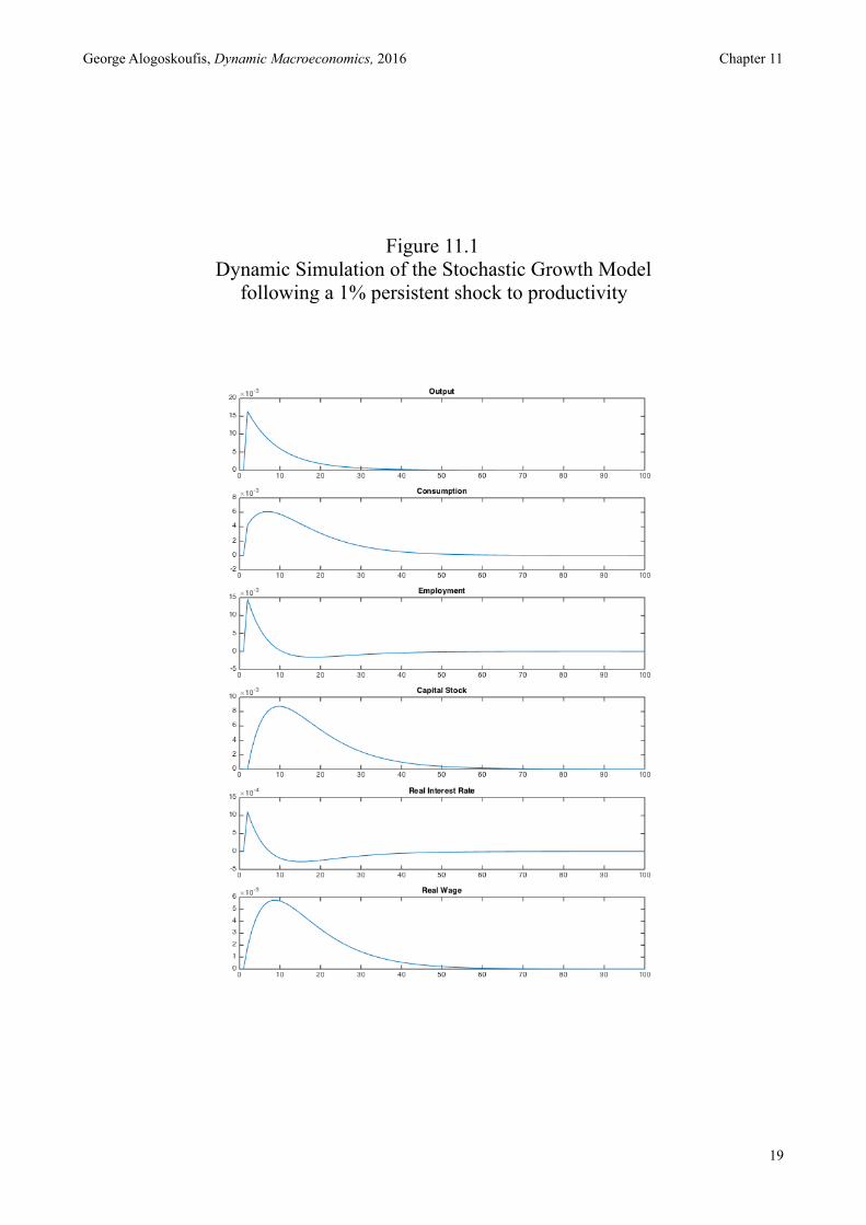
In Figure 11.1 we present the results of a dynamic simulation of the model, for a 1% positive shock in productivity a. The parameter values we used in the simulation were α=0.333, ρ=0.02, g=0.02, δ=0.03, ν=2, ηA=0.90.

As can be seen from the simulated impulse response functions, all real variables move pro-cyclically, as innovations in productivity affect output, the capital stock, consumption and employment in the same direction. Real wages and the real interest rate also move pro-cyclically. Gradually, all variables converge to the steady state unless the system is disturbed by another shock.

yt = (ηKK +ηA )yt−1 −ηKKηAyt−2 + (1−α )(1+ηLA )ε tA − (1−α ) ηKK (1+ηLA )−ηLKηKA( )ε t−1A

!18


Figure 11.1 Dynamic Simulation of the Stochastic Growth Model

following a 1% persistent shock to productivity

!19


References

Alogoskoufis G. (1983), “The Labour Market in an Equilibrium Business Cycle Model”, Journal of Monetary Economics, 11, pp. 117-128.

Alogoskoufis G. (1987a), “On Intertemporal Substitution and Aggregate Labor Supply”, Journal of Political Economy, 95, pp. 938-960.

Alogoskoufis G. (1987b), “Aggregate Employment and Intertemporal Substitution in the UK”, The Economic Journal, 97, pp. 403-415.

Barro R.J. (1976), “Rational Expectations and the Role of Monetary Policy”, Journal of Monetary Economics, 2, pp. 1-32.

Bernanke B.S. (2006), “Monetary Aggregates and Monetary Policy at the Federal Reserve: A Historical Perspective”, Speech at the 4th ECB Central Banking Conference, Frankfurt, Board of Governors of the Federal Reserve System.

Campbell John Y. (1994), “Inspecting the Mechanism: An Analytical Approach to the Stochastic Growth Model”, Journal of Monetary Economics, 33, pp. 463-506.

Fisher I. (1896), Appreciation and Interest, Publications of the American Economic Association, 11, pp. 1-98.

Fisher I. (1930), The Theory of Interest, New York, Macmillan. Gali J. (2008), Monetary Policy, Inflation and the Business Cycle, Princeton N.J., Princeton

University Press. King R.G. and Rebelo S.T. (1999), “Resuscitating Real Business Cycles”, in Taylor J.B. and

Woodford M. (1999), Handbook of Macroeconomics, Vol. 1B, Amsterdam, Elsevier. Kydland F.E. and Prescott E.C. (1982), “Time to Build and Aggregate Fluctuations”, Econometrica,

50, pp. 1345-1370. Long J.B. and Plosser C.I. (1983), “Real Business Cycles”, Journal of Political Economy, 91, pp.

39-611. Lucas R.E. Jr (1972), “Expectations and the Neutrality of Money”, Journal of Economic Theory, 4,

pp. 103-124. Lucas R.E. Jr (1973), “Some International Evidence on Output-Inflation Tradeoffs”, American

Economic Review, 63, pp. 326-334. Lucas R.E. Jr (1976), “Econometric Policy Evaluation: A Critique”, Carnegie Rochester

Conference Series on Public Policy, 1, pp. 19-46. Lucas R.E. Jr (1977), “Understanding Business Cycles”, Carnegie Rochester Conference Series on

Public Policy, 5, pp. 7-21. Lucas R.E. Jr and Rapping L. (1969), “Real Wages, Employment and Inflation”, Journal of

Political Economy, 77, pp. 721-754. McCallum B.T. “Price Level Determinacy with an Interest Rate Policy Rule and Rational

Expectations”, Journal of Monetary Economics, 8, pp. 319-329. Poole W. (1970), “Optimal Choice of Monetary Policy Instruments in a Simple Stochastic Macro

Model”, The Quarterly Journal of Economics, 84, pp. 197-216. Prescott E.C. (1986), “Theory Ahead of Business Cycle Measurement”, Carnegie-Rochester

Conference Series on Public Policy, 25, pp. 11-44. Ramsey F. (1928), “A Mathematical Theory of Saving”, Economic Journal, 38, pp. 543-559. Sargent T.J. (1976), “A Classical Macro-econometric Model for the United States”, Journal of

Political Economy, 84, pp. 207-238. Sargent T.J. and Wallace N. (1975), “Rational Expectations, the Optimal Monetary Instrument and

the Optimal Money Supply Rule”, Journal of Political Economy, 83, pp. 241-254.

!20


Wicksell K. (1898), Interest and Prices, (English translation, Kahn R.F. 1936), London, Macmillan. Woodford M. (2003), Interest and Prices: Foundations of a Theory of Monetary Policy, Princeton

N.J., Princeton University Press.

!21

chapter 11 the stochastic growth model and aggregate ... · chapter 11 the stochastic growth model...

Documents