chapter 11 representation & description
TRANSCRIPT

Image Comm. Lab EE/NTHU 1
Chapter 11Representation & Description
• Image segmented into regions, how to represent and describe these regions?
1) In terms of its external characteristics (boundary)
2) In terms of its internal characteristics (pixels in the region)

Image Comm. Lab EE/NTHU 2
11.1 Representation – Chain code
• Chain codes are used to represent a boundary as a connected sequence of straight line segments of specified length and direction.
• The representation is based on 4- or 8- connectivity. • Chain code is generated by following a boundary in
clockwise direction and assigning a direction to the segments connecting every pair of pixels.
• Disadvantages of chain codes:1) The chain code is quite long2) Any small disturbance along the boundary due to
noise cause change in the code that may not related to the shape of the boundary.

Image Comm. Lab EE/NTHU 3
11.1 Representation – Chain code11.1 Representation – Chain code

Image Comm. Lab EE/NTHU 4
11.1 Representation – chain code
11.1 Representation – chain code

Image Comm. Lab EE/NTHU 5
11.1 Representation – Chain code
• The chain code of a boundary depends on the starting point.
• Normalize the chain code by using the first difference of the chain code.
• Example: the chain code is 10103322,the first difference is 3133030 or 33133030, the 1st “3” is obtained by connecting the last and the first element of the chain.
• Size normalization can be obtained by alternating the size of the sampling grid.

Image Comm. Lab EE/NTHU 6
11.1 Representation - Polygon approximation
• Minimum perimeter polygons– Enclose the boundary by a set of concatenated cells
(Fig. 11.3).– The enclosure has two walls corresponding to the
inside and outside boundaries of the strip of cell.– Think of the object boundary as a rubber band
contained within the wall.– The rubber band shrinks and produces a polygon of
minimum perimeter that fit the geometry established by the cell strip.

Image Comm. Lab EE/NTHU 7
11.1 Representation - Polygon approximation11.1 Representation - Polygon approximation
Image Comm. Lab EE/NTHU 8
11.1 Representation - Polygon approximation
• Merging technique– Merge points along the boundary until the
least square error line fit of the points merged so far exceeds a preset threshold.
– Difficulties: the vertices do not always correspond to inflections (corners) in the original boundary.

Image Comm. Lab EE/NTHU 9
11.1 Representation Polygon approximation
• Splitting techniques:• Subdivide a segment successively into two parts until a
specified criterion is satisfied.• The maximum perpendicular distance from a boundary
segment to the line joining its two end points not exceed a preset threshold.
• If it does, the farthest point from the line become a vertex, thus subdivide the segment into two sub-segments,
• This approach has the advantage in seeking prominent inflection points

Image Comm. Lab EE/NTHU 10
11.1 Representation - Polygon approximation11.1 Representation - Polygon approximation

Image Comm. Lab EE/NTHU 11
11.1 Representation - Polygon approximation
• Signature• 1-D functional representation of a boundary.
1) Plot the distance from the centroid to the boundary as a function of angles (Fig. 11.5), i. e., r(θ).– Invariant to translation, but depend on the rotation and scaling.– Normalizing with respect to rotation.– Select the starting point as the point farthest to the centroid.
2) Traverse the boundary and plot the angle between a line tangent to the boundary at that point and a reference line. Then use the Slope density function: (histogramof tangent-angle values) as signature.

Image Comm. Lab EE/NTHU 12
11.1 Representation - Polygon approximation11.1 Representation - Polygon approximation

Image Comm. Lab EE/NTHU 13
11.1 Representation-boundary segment
• Convex hull H of an arbitrary set S is the smallest convex set containing S.
• The difference H–S is call convex deficiency D of the set S.
• The region boundary can be partitioned by following the contour of S and marking the points at which a transition is made into or out of a component of the convex deficiency.
• The concept of convex hull and its deficiency are equally useful for describing an entire region, as well as just its boundary.

Image Comm. Lab EE/NTHU 14
11.1 Representation-boundary segment11.1 Representation-boundary segment

Image Comm. Lab EE/NTHU 15
11.1 Representation - Polygon approximation
• Skeleton of a region can be obtained by thinning algorithm
• Medial axis transformation (MAT):1) For each point in region R, we find its closest neighbor in
border B.2) If p has more than one such neighbor, it is said to belong to
the medial axis (skeleton) of R.• Thinning algorithm: iteratively delete the edge points
of a region subject to1) Does not remove the end points2) Does not break connectivity3) Does not cause excessive erosion of the region.

Image Comm. Lab EE/NTHU 16
11.1 Representation - Polygon approximation 11.1 Representation - Polygon approximation

Image Comm. Lab EE/NTHU 17
11.1 Representation - Polygon approximation 11.1 Representation - Polygon approximation

Image Comm. Lab EE/NTHU 18
11.1 Representation - Polygon approximation
• Thinning algorithmStep 1) flag a contour point p1 for deletion if the
following conditions are satisfied:a) 2≤N(p1)≤6, where N(p1) is the number of neighbors of p1.b) T(p1)=1, where T(p1) is number of 0-1 transitions in the
ordered sequence p2, p3,….. p8, p9, p2c) p2•p4•p6=0d) p4•p6•p8=0If all conditions are satisfied, the point is flagged for deletion.
Step 2) Conditions (c) and (d) changed toc’) p2•p4•p8=0d’) p2•p6•p8=0

Image Comm. Lab EE/NTHU 19
11.1 Representation - Polygon approximation
• Thinning algorithm1) Apply step 1 to flag border points for deletion2) Deleting the flagged point3) Apply step 2 to flag the remaining border points for
deletion.4) Delete the flagged pointsThe basic procedure is applied iteratively until no further points
are deleted.• Condition (a) is violated when p1 is the end point of
a skeleton stroke.• Condition (b) is violated when it is applied to points
on stroke 1 pixel thick.

Image Comm. Lab EE/NTHU 20
11.1 Representation - Polygon approximation 11.1 Representation - Polygon approximation
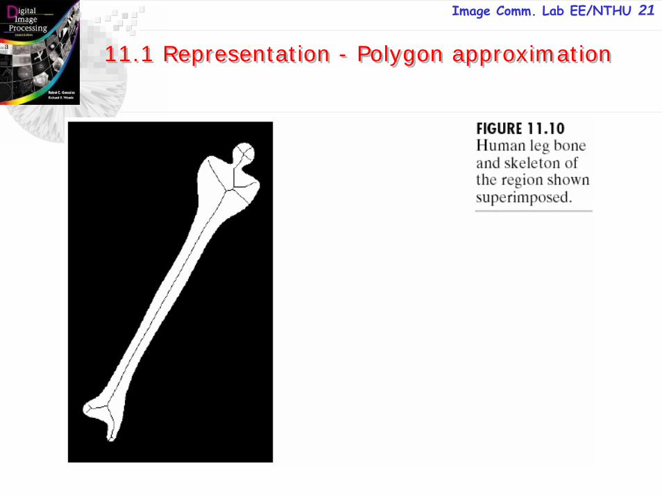
Image Comm. Lab EE/NTHU 21
11.1 Representation - Polygon approximation 11.1 Representation - Polygon approximation

Image Comm. Lab EE/NTHU 22
11.2 Boundary descriptor
• Simple descriptors1) Length2) Diameter: Diam(B)=max[D(pi, pj)] where pi and pj
are points on the boundary. 3) Major axis and minor axis4) Basic rectangle5) Eccentricity = major axis/minor axis6) Curvature: changes of slope.7) Point p belongs to a segment which is convex if the
change of slope at p is nonnegatoive and concave otherwise.
8) P is a corner depends on the curvature.

Image Comm. Lab EE/NTHU 23
11.2 Boundary Description - shape number
• The first difference of a chain-coded boundary depends on the starting point.
• The shape number of a chain coded boundary is defined as the first difference of smallest magnitude.
• The difference of a chain code is independent of it rotation, it depend on the orientation of the grid.
• The order n of a shape number is defined as the number of digits in its representation.

Image Comm. Lab EE/NTHU 24
11.2 Boundary Description- shape number11.2 Boundary Description- shape number

Image Comm. Lab EE/NTHU 25
11.2 Boundary Description- shape number
• Example (Fig. 11.12)• 1. Find the basic rectangle for n=18 (boundary)• 2. Find the major and minor axis• 3. Find the closest rectangle of order 18 is 3x6 • 4. obtain chain code• 5. find the difference• 6. find the shape no.

Image Comm. Lab EE/NTHU 26
11.2 Boundary Description
11.2 Boundary Description

Image Comm. Lab EE/NTHU 27
11.2 Boundary Description–Fourier Descriptor
• For a K-point digital boundary, starting at an arbitrary point (x0, y0), K coordinate pairs (x0, y0), (x01, y01), ….,(xK-1, yK-1) are encountered in counterclockwise direction.
• Let s(k)=[x(k), y(k)] for k=0,1,….K-1, or s(k)=x(k)+jy(k)
• The 1-D DFT of s(k) is
• The inverse DFT of a(u) is
∑−
=
−=1
0
/2)(1)(K
k
KukjeksK
ua π
∑−
=
=1
0
/2)(1)(K
k
KukjeuaK
ks π

Image Comm. Lab EE/NTHU 28
11.2 Boundary Description- Fourier Descriptor11.2 Boundary Description- Fourier Descriptor

Image Comm. Lab EE/NTHU 29
11.2 Boundary Description - Fourier Descriptor
• If only the first P coefficients (P<K) are used then
• The coefficients {a(u)} carry shape information which are insensitive to translation, rotation, and scale change of the shape.
• The descriptors are insensitive to the change of starting point.• Rotation of a point by an angle θ about the origin of the complex
plane is accomplish by multiplying the point by ejθ .• The rotated sequence s(k)ejθ whose Fourier descriptors are
∑−
=
=1
0
/2)()(ˆP
u
Kukjeuaks π
θπθ jK
k
Kukjjr euaeeks
Kua )()(1)(
1
0
/2 == ∑−
=
−

Image Comm. Lab EE/NTHU 30
11.2 Boundary Description - Fourier-Descriptor11.2 Boundary Description - Fourier-Descriptor

Image Comm. Lab EE/NTHU 31
11.2 Boundary Description-Fourier-Descriptor
11.2 Boundary Description-Fourier-Descriptor
1) Translation: st(k)=s(k)+Δxy=[x(k)+Δx]+j[y(k)+Δy]
2) Change the starting point of the sequence to k=k0 from k=0 as
sp(k)=s(k-k0)=x(k-k0)+j y(k-k0)

Image Comm. Lab EE/NTHU 32
The contour of hand silhouette.
11.2 Boundary Description – Fourier Descriptor11.2 Boundary Description – Fourier Descriptor

Image Comm. Lab EE/NTHU 33
• Fourier series of a sequence of points {x(m),y(m)} can be defined as
where a(n) and b(n) are the Fourier coefficient
11.2 Fourier Descriptor
∑= Nnmjenam)x /2)(( π ∑= Nnmjenbm)y /2)(( π
∑=
−=N
m
Nnmjemxna1
/2)()( π ∑=
−=N
m
Nnmjemynb1
/2)()( π

Image Comm. Lab EE/NTHU 34
11.2 Fourier Descriptor
• Assuming local variation of hand shape is smooth so that the higher order terms of the Fourier descriptor are not necessary.
• To normalize the size of hand gesture we let S(n)=r(n)/r(1) (normalization), and we have
• Using 22 harmonics of the FD’s coefficient, S(n), is enough to describe the macroscopic information of the hand shape.
• FD is translation, rotation, and scaling invariance.
22 |b(n)||a(n)|r(n) += n=1,2,….,22

Image Comm. Lab EE/NTHU 35
11.2 Fourier Descriptor

Image Comm. Lab EE/NTHU 36
11.2 Boundary Description-Statistical moment
• The shape of boundary segments can be described quantitatively by using simple statistical moments such as mean, variance, and higher-order moments.
• Figure 11.5 represented as 1-D function g(r).• Treat the amplitude of g as a discrete random
variable v and form an amplitude histogram p(vi), i=0,1,…A-1, where A is the number of discrete amplitude increments in which we divide the amplitude scale.

Image Comm. Lab EE/NTHU 37
11.2 Boundary Description-Statistical moment
11.2 Boundary Description-Statistical moment

Image Comm. Lab EE/NTHU 38
11.2 Boundary Description-Statistical moment
• The nth moment of v about its mean m is
where the mean is
• The m is the mean and μ2 is the variance.
∑−
=
=1
0)(
A
iii vpvm
∑−
=
−=1
0)()()(
A
ii
nin vpmvvμ

Image Comm. Lab EE/NTHU 39
11.2 Boundary Description-Statistical moment
• An alternative approach is normalize g(r) to unit area and treat it as histogram.
• g(ri) is treated as the probability of value rioccuring.
• The moments are
where ∑−
=
=1
0)(
K
iii rgrm
∑−
=
−=1
0)()()(
K
ii
nin rgmrrμ

Image Comm. Lab EE/NTHU 40
11.3 Regional Descriptors-Simple Descriptor
• Area is the number of pixels in the regions• Perimeter is the length of the boundary.• Compactness=(perimeter)2/area.

Image Comm. Lab EE/NTHU 41
11.3 Regional Descriptors11.3 Regional Descriptors

Image Comm. Lab EE/NTHU 42
11.3 Regional Descriptors -Topological Descriptor
• Topology is the study of properties of a figure that are unaffected by any deformation (rubber-sheet distortion).
• The number of holes: H• The number of connected components: C• Euler number E: E=C-H.

Image Comm. Lab EE/NTHU 43
11.3 Regional Descriptors -Topological Descriptor
11.3 Regional Descriptors -Topological Descriptor

Image Comm. Lab EE/NTHU 44
11.3 Regional Descriptors -Topological Descriptor
• Regions represented by straight-line segments (polygonal networks), such as Fig. 11.20, has the following relationship intopology as
E=V-Q+F=C-Hwhere V is the number of vertices and Q is the number of edges.
• Segmentation is based on the thresholding.• How the connected components can be used to “finish” the
segmentation.• Figure 11.21(b) has 1591 connected components, C=1591, and
its Euler number E=1552, and H=39. Figure 11.21(c) shows the connected component with 8479 elements

Image Comm. Lab EE/NTHU 45
11.3 Regional Descriptors -Topological Descriptor11.3 Regional Descriptors -Topological Descriptor
V-Q+F = C-H = E
7-11+2 = 1-3 = -2

Image Comm. Lab EE/NTHU 46
11.3 Regional Descriptors -Topological Descriptor11.3 Regional Descriptors -Topological Descriptor

Image Comm. Lab EE/NTHU 47
11.3 Regional Descriptors -Texture
• The texture measurement provides the properties such as smoothness, coarseness, and regularity.
• Three principal approaches: statistical, structure, and spectral.• Statistical approaches:
Let z be a random variable and p(zi), i=0,1,…L-1 is the corresponding histogram, L is the number of gray-levels.
The nth moment of z about the mean (m) is
The second moment μ2 (=varianceσ2) can be used to define the measure R as
R=0 (for constant density, σ=0), R→1 (for large σ)
∑−
=
−=1
0)()()(
L
ii
nin zgmzzμ
)(111 2 z
Rσ+
−=

Image Comm. Lab EE/NTHU 48
11.3 Regional Descriptors -Texture
• Statistical approachThe 2nd moment μ2 (=varianceσ2) is used to measure the contrast.The 3rd moment μ3 is used to measure the skewness of the
histogram.The 4th moment μ4 is used to measure the relative flatness of the
histogram.The measure of “uniformity” of the histogram as
The average entropy measure as
This approach measure no information regarding to the relative position of pixels with respect to each other.
∑−
=
=1
0
2 )(L
iizpU
∑−
=
−=1
02 )(log)(
L
iii zpzpe

Image Comm. Lab EE/NTHU 49
11.3 Regional Descriptors -Texture11.3 Regional Descriptors -Texture

Image Comm. Lab EE/NTHU 50
11.3 Regional Descriptors -Texture11.3 Regional Descriptors -Texture

Image Comm. Lab EE/NTHU 51
11.3 Regional Descriptors -Texture
• Let P be a position operator, A be a k×k matrix whose element aij is the number of times that points with gray level zi,occur (in position specified by P) relative to points with gray level zj, with 1≤i, j ≤k.
• For example, an image with z1=0, z2=1, z3=2 as• Define the position operator P as “one pixel below
and one-pixel to the right yields a 3×3 matrix A as• a11 is the number of times that a point with level
z1=0 appears related with another point of the same level
• a13 is the number of times that a point with level z1=0 appears related with another point with gray-level z3=2
1010002011001221101121000
⎥⎥⎥
⎦
⎤
⎢⎢⎢
⎣
⎡=
020232124
A

Image Comm. Lab EE/NTHU 52
11.3 Regional Descriptors -Texture
• Let n be the number of point pairs in the image that satisfy P (n=16).
• If C=A/n then cij is the estimate of the joint probability that a pair of points satisfying P will have values (zi, zj)
• The matrix C is called gray-level co-occurence matrix.• C depends on P.• To analyze a given C to categorize the texture of
region over which C was computed.

Image Comm. Lab EE/NTHU 53
11.3 Regional Descriptors -Texture
• A set of descriptors based on C are1) Maximum probability2) Element difference moment of order k3) Inverse element difference moment of order k4) Uniformity5) Entropy

Image Comm. Lab EE/NTHU 54
11.3 Regional Descriptors -Texture
• Structural approach: a simple “texture” primitive can be used to form more complex texture pattern.
1) Define a rule of the form : S→ aS, which indicates that the symbol S may be written as aS.
2) Let a represents a circle, and the meaning of “circles to the right” is assign a string of the form aaa..., and the rule S→ aS generates Fig11.23(b).
3) Define new rules: S→ bA, A→ cA, A→ c, A→ bS, S→ a, where b represents “circle down” and c means “circle to the left”
4) Generate a string of the form aaabccbaa that corresponding to a 3×3 matrix of circles.

Image Comm. Lab EE/NTHU 55
11.3 Regional Descriptors -Texture11.3 Regional Descriptors -Texture

Image Comm. Lab EE/NTHU 56
11.3 Regional Descriptors -Texture
• Spectral approach• Fourier spectrum is suitable for describing the
directionality of periodic in 2-D image.• Three features in Fourier spectrum:
1) Prominent peaks give the principal direction of the texture patterns.
2) The location of the peaks give the fundamental spatial period of the patterns.
3) By filtering the periodic component, the other non-periodic pattern can be described by statistical technique.

Image Comm. Lab EE/NTHU 57
11.3 Regional Descriptors -Texture
• Spectral approach• Express the spectral in polar coordinates as S(r, θ).• For each direction θ, we have a 1-D expression of the
spectrum as Sθ(r). • Global description as S(r)=Σθ Sθ(r). • For each frequency r, we have a 1-D expression of the
spectrum as Sr(θ). • Global description as S(θ)=Σr Sr(θ). • Constitute [S(r),S(θ)] for each pair of (r, θ)

Image Comm. Lab EE/NTHU 58
11.3 Regional Descriptors -Texture11.3 Regional Descriptors -Texture
S(r)

Image Comm. Lab EE/NTHU 59
11.3 Regional Descriptors -Texture
• Moment of two dimensional functions• For 2-D continuous function f(x, y), the moment of order (p+q)
is defined as
• The central moments are
. orwhere = m10/m00 and = m01/m00
The central moments are μ00,(=m00), μ10 (=0),μ01(=0), μ11, μ20, μ02, μ21, μ12,…..
∑∑∫ ∫ ==∞
∞−
∞
∞−x y
qpqppq yxfyxdxdyyxfyxm ),(),(
∫ ∫∞
∞−
∞
∞−−−= dxdyyxfyyxx qp
pq ),()()(μ
∑∑ −−=x y
qppq yxfyyxx ),()()(μ
x y
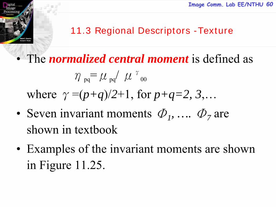
Image Comm. Lab EE/NTHU 60
11.3 Regional Descriptors -Texture
• The normalized central moment is defined as ηpq=μpq/ μγ
00
where γ=(p+q)/2+1, for p+q=2, 3,…• Seven invariant moments Φ1, …. Φ7 are
shown in textbook• Examples of the invariant moments are shown
in Figure 11.25.

Image Comm. Lab EE/NTHU 61
11.3 Regional Descriptors -Texture
11.3 Regional Descriptors -Texture

Image Comm. Lab EE/NTHU 62
11.3 Regional Descriptors -Texture11.3 Regional Descriptors -Texture

Image Comm. Lab EE/NTHU 63
11.4 Use of Principal Component Description
• Treat the vectors x as a random quantity.• The mean vector is mx=E{x}• The covariance matrix: Cx=E{(x–mx)(x– mx)T}
which is real and symmetric.• cii is variance of xi, and cij is the covariance between
elements xi and xj .• If element xi and xj are uncorrelated then cij=cji=0.

Image Comm. Lab EE/NTHU 64
11.4 Use of Principal Component Description
• For K vector samples from random population, the mean vector is
• By expanding the product (x–mx)(x–mx)T, the covariance matrix can be approximated as
∑=
=K
kkx K 1
1 xm
∑=
−=K
k
Tkk
Tkkx K 1
1 mmxxC

Image Comm. Lab EE/NTHU 65
11.4 Use of Principal Component Description
• Example 11.9. x1=[0, 0, 0]T, x2=[1, 0, 0]T x3=[1, 1, 0]T x4=[1, 0, 1]T .
• We may compute mx and Cx as
mx=1/4[3, 1, 1]T
• The diagonal terms indicate that the three components of the vectors have the same variance.
• x1 and x2, x1 and x3 are positive related.• x2 and x3 are negative related.
⎥⎥⎥
⎦
⎤
⎢⎢⎢
⎣
⎡
−−=311131
113
161
xC

Image Comm. Lab EE/NTHU 66
11.4 Use of Principal Component Description
• Because Cx is real and symmetric, we may find a set of n orthonormal eigenvectors.
• Let ei and λi, i=1, 2,…n be the eigenvectors and eigenvalues of Cx, with λi≥λi+1.
• Let A be the matrix whose rows are formed from the eigenvectors of Cx ordered so that the first row of Ais eigenvector corresponding to the largest eigenvalue, and the last row is the eigenvector corresponding to the smallest eigenvalue.
• Suppose A is used as a transformation matrix to map the x’s into vector denoted by y’s as follows:
y=A(x-mx)

Image Comm. Lab EE/NTHU 67
11.4 Use of Principal Component Description
• The above expression is called Hotelling transform or Principal component transform.
• my=E{y}=0• Cy is=ACxAT.• Cy is a diagonal matrix.
• The reconstruction of x is x=ATy+mx
⎥⎥⎥⎥⎥⎥
⎦
⎤
⎢⎢⎢⎢⎢⎢
⎣
⎡
=
nλ
λλ
0.
.
01
2yC

Image Comm. Lab EE/NTHU 68
11.4 Use of Principal Component Description
• Instead of using all eigenvectors of Cx, we form matrix Ak from k eigenvector corresponding to klargest eigenvalues.
• Ak is a transformation matrix of order kxn.• The y vector would be k dimension.• The reconstructed vector is no longer exact as
xmyAx += Tkˆ

Image Comm. Lab EE/NTHU 69
11.4 Use of Principal Component Description11.4 Use of Principal Component Description

Image Comm. Lab EE/NTHU 70
11.4 Use of Principal Component Description11.4 Use of Principal Component Description

Image Comm. Lab EE/NTHU 71
11.4 Use of Principal Component Description
11.4 Use of Principal Component Description

Image Comm. Lab EE/NTHU 72
11.4 Use of Principal Component Description11.4 Use of Principal
Component Description

Image Comm. Lab EE/NTHU 73
11.4 Use of Principal Component Description11.4 Use of Principal
Component Description

Image Comm. Lab EE/NTHU 74
11.5 Relational Description
• Rules for describing the context of relation.• Apply equally to boundaries and regions.• Define two primitives a and b as shown in Fig. 11.30.• We define rewriting rules as
(a) S→aA(b) A→bS(c) A→b.where A and S are variables, and the elements a and b are constant corresponding o the primitives.
Rule 1 indicates the staring symbols S can be replaced by aA.

Image Comm. Lab EE/NTHU 75
11.5 Relational Description11.5 Relational Description
Let A and S are variables, define rewriting rules as
(a) S→aA
(b) A→bS
(c) A→b.

Image Comm. Lab EE/NTHU 76
11.5 Relational Description11.5 Relational Description
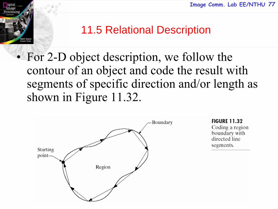
Image Comm. Lab EE/NTHU 77
11.5 Relational Description
• For 2-D object description, we follow the contour of an object and code the result with segments of specific direction and/or length as shown in Figure 11.32.

Image Comm. Lab EE/NTHU 78
11.5 Relational Description
• Another description is to describe the sections of an image (small homogeneous region) by direct line segments, which can be joined in other ways besides head-to-tail connections as shown in Figure 11.33.
• Sting descriptions are best suited for applications in which connectivity of primitives can be expressed in a head-to-tail or other connected manner.

Image Comm. Lab EE/NTHU 79
11.5 Relational Description11.5 Relational Description
Image Comm. Lab EE/NTHU 80
11.5 Relational Description
• Sometimes regions may not be contiguous, and we use Tree to describe such regions.
• A tree T is a finite set of one or more nodes for whicha) there is a unique node $ designated the rootb) the remaining nodes are partitioned into m disjoint sets T1, ….Tm, each of which in turn is a tree called a subtree of T.
The tree frontier is a set of nodes at the bottom of the tree (the leaves), taken in order from left to right, (see Figure 11.34).

Image Comm. Lab EE/NTHU 81
11.5 Relational Description
Two types of information in a treea) information about a nodeb) information relating a node to its neighbors
For image description, the 1st type of information identifies an image structure, whereas the 2nd
type of information defines the physical relationship of that substructure to other substructure.

Image Comm. Lab EE/NTHU 82
11.5 Relational Description11.5 Relational Description