chapter 11 - cleveland state universitycis.csuohio.edu/~sschung/cis611/enach11-further...successive...

1

Copyright © 2007 Pearson Education, Inc. Publishing as Pearson Addison-Wesley

Chapter 11

Relational Database Design

Algorithms and Further

Dependencies

Copyright © 2007 Pearson Education, Inc. Publishing as Pearson Addison-Wesley Slide 11- 2

Decompositions

Definition

The decomposition of a schema R=A1…An is its replacement by a collection

DR = {R1, R2, …, Rm} of subsets of R such that R = R1 R2 … Rm

Note: schemas Ri‟s do not have to be disjoint!

Example 1

Assume the schema R=ABCD. The following are possible decompositions

of R.

D1 = {AB, CD}

D2 = {AB, ACD}

D3 = {A, BCD}

D4 = {AB, BC, CD, AD}

2


Dependency Preservation Property of a Decomposition

Observations• It would be useful if each functional dependency X→Y specified in F either

appeared directly in one of the relation schemas Ri in the decomposition or

could be inferred from the dependencies that appear in some Ri.

• We want to preserve the dependencies because each rule in F represents a

constraint on the database.

• If one of the dependencies is not represented in some individual relation Ri of

the decomposition, we cannot enforce this constraint by dealing with an

individual relation. We may have to join multiple relations so as to include all

attributes involved in that dependency.

• It is not necessary that the exact dependencies specified in F appear themselves

in individual relations of the decomposition D. It is sufficient that the union of

the dependencies that hold on the individual relations in D be equivalent to F.

Copyright © 2007 Pearson Education, Inc. Publishing as Pearson Addison-Wesley Slide 11- 4Slide 11- 4


Definition

Given a set of dependencies F on R, the projection of F on Ri, denoted by Ri(F) where Ri is a subset of R, is the set of dependencies X → Y in F+ such

that the attributes in X Y are all contained in Ri.

Hence, the projection of F on each relation schema Ri in the

decomposition D is the set of functional dependencies in F+

such that all their left- and right-hand-side attributes are in Ri.

We say that a decomposition D = {R1, R2, . . . , Rm} of R is

dependency-preserving with respect to F if the union of the projections of F on

each Ri in D is equivalent to F; that is,

( R1(F) R2(F) . . . Rm(F) )+= F+

3



Claim

It is always possible to find a dependency-preserving decomposition D

with respect to F such that each relation is in 3NF (to be discussed later).

Example 2a

Assume R= ABCD, and F= {A→B, C → D}. The decomposition

D1 = {AB, CD} is clearly F-preserving. Observe the first rule is kept in R1,

while the second is preserved in R2. Also notice that schemas AB and CD

are in 3NF format.

A B C D F= {A→B, C → D}

A B C D

F2= {C → D}F1= {A→B}



Example 2b

Assume R= ABCD, and F= {A→B, B →C, C → D}. Evaluate the

decomposition D = {ABC, CD}.

D is clearly F-preserving. Observe that

F1 = ABC(F)= {A→B, B →C} and

F2 = CD(F)= {C→D}

and F = F1 F2

4



Algorithm: Testing Preservation of Functional Dependencies

Input: A set F of FDs on schema R, a partition D = (R1 . . .Rm) of R, and a dependency X→Y with R XY.

Output: true whenever the dependency X→Y is retained by the decomposition D, i.e. (Ri F) X→Y, and false otherwise

Method: beginZ = X;while changes to Z occur do

for i =1 to m doZ = Z [ ( Z ∩ Ri )+F ∩ Ri ];

if ( Z Y )

then return (true)else return (false);

end;



Example 2c. source Ullman, J. "Database Systems", Computer Sc. Press

Consider schema R=ABCD, D = {R1= AB, R2= BC, R3= CD }

subjected to F = { A→B, B→C, C→D, D→A }.

Question: Is D→A lost in the projections?

Answer: Even though there is no segment containing attributes DA the rule D→A is not lost ( ZD= ABCD A ).

Why? Let‟s use the F-Preserving Test Algorithm. If D preserves F it must occur that R1(F) R2(F) R3(F) D→A. Observe that the other three

rules in F are naturally retained in R1, R2, and R3.

Let‟s begin with Z = D ( this the LHS of D→A )1. Use R1= AB. Here Z= D [( D ∩ AB)+ ∩ AB] = D

2. Use R2= BC. Here Z= D [( D ∩ BC)+ ∩ BC] = D

3. Use R3= CD. Here Z= D [( D ∩ CD)+ ∩ CD] = DC (a change! ) …

4. Use R2= BC. Here Z= D [( DC ∩ BC)+ ∩ BC] = DCB (a change! ) …

5. Use R1= AB. Here Z= DCB [( DCB ∩ AB)+ ∩ AB] = DCBA A. Stop! Rule is kept in D

Skipping some steps

Of the iteration

5



Example 2c (cont). source Ullman, J. "Database Systems", Computer Sc. Press

Consider schema R=ABCD, D = {R1= AB, R2= BC, R3= CD }

subjected to F = { A→B, B→C, C→D, D→A }.

Observation:

The rule D→A is preserved in the decomposition (R1, R2, R3)

Although not obvious it is clear that the following FDs are in F+

F + ⊇ { A→B, B→C, C→D, D→A, B →A, C →D, D →C }

Therefore

F1 = { A→B, B →A } on R1=(AB)

F2 = { B→C, C →B } on R2=(BC)

F3 = { C→D, D →C } on R3=(CD)

Finally(F1 F2 F3)+ derives the FD D →A and consequently it is not lost.


Nonadditive (Lossless) Join Property of a Decomposition

Observation

Another property that a decomposition D should possess is the

nonadditive join property, which ensures that no spurious (phantom)

tuples are generated when a NATURAL JOIN operation is applied to

the relations in the decomposition

Definition.

Formally, a decomposition D = {R1, R2, . . . , Rm} of R has the lossless

(nonadditive) join property with respect to the set of dependencies F on

R, if for every relation state r of R that satisfies F, the following holds,

where * is the NATURAL JOIN of all the relations in D: *(R1(r) ,. . , Rm(r)) = r.

The word loss in lossless refers to loss of information, not to loss of tuples. If a decomposition

does not have the lossless join property, we may get additional spurious tuples

The nonadditive join property ensures that no spurious tuples result after the application of

PROJECT and JOIN operations.

6


Nonadditive Lossless-Join Decomposition

Example 3

Schema < R=ABC , F = { A→B }> and partition D2 = { AB, BC }

Consider the decompositions

D1 = { AB, AC } and

D2 = { AB, BC }

Observe that D1 is a „good‟

decomposition (lossless) while

D2 is not.

Phantom /Spurious rows created

when using decomposition D2

D2



Example 3 cont.

Schema < R=ABC , F = { A→B }> and partition D1 = { AB, AC }

Consider the decompositions

D1 = { AB, AC } and

D2 = { AB, BC }

Observe that D1 is a „good‟

decomposition (lossless)

while D2 is not.

Notice that r’ = AB(r) * AC(r)

D1

7



Example 3 cont.

Schemas < R1= ABC, F1 = { A→BC, C →B } > and

< R2= BCD, F2 = { C →B, B →C, D →B }

Observe that r1 r1‟

r1 tuple <2,2,6> is lost in

the JOIN and does not

appear in r1‟

D1


Testing Lossless-Join (or Non-Additive) Decomposition

Definition (good only on binary partition)

If D={ R1, R2 } is a decomposition of R and F is a set of FDs on R, then D has

a lossless-join with respect to F if

F ( R1 R2) → (R1 - R2) or F ( R1 R2) → (R2 – R1)

Example 4

Consider the previous problem where R=ABC and F = { A→B }.

Let‟s assess the partition D1 = {AB, AC}. Here R1=AB and R2= ACtherefore R1 R2 = A

R1 – R2 = B

R2 – R1 = C

The question F ( R1 R2) → (R1 - R2) is equivalent to FA → B and we

know this is true because F contains exactly this dependency.

We must conclude the decomposition D1 is lossless with respect to F.

8



Example 4 (continuation)

Consider the previous problem where R=ABC and F = { A→B }.

Let‟s now evaluate the partition D2 = {AB, BC}.

Here R1=AB and R2= BC

therefore R1 R2 = B

R1 – R2 = A

R2 – R1 = C

The question F ( R1 R2) → (R1 - R2) is equivalent to F B → A (or

F B → C). Both dependencies are NOT derivable from F (they are not

in F+).

We conclude the decomposition D2 is NOT lossless with respect to F (we

will call it a lossy decomposition).


Example 5

Consider the schema R=ABCD and F = { A→B, C→D }.

Let‟s now evaluate the following binary partitions

R1 R2 R1 – R2 R2 – R1

1 = {AB, CD} AB CD No

2 = {AC, BCD} C A BD No (neither C →A

nor C →BD in F+)

3 = {ABC, CD} C AB D Yes C→D in F+

2 = {BD, ACD} D B AC No

We conclude only the decomposition 3 is lossless with respect to F.


9


Successive (Non-Additive) Lossless-Join Decompositions

Claim.

If a decomposition D = {R1, R2, . . . , Rm} of R has the nonadditive

(lossless) join property with respect to a set of functional dependencies F

on R, and if a decomposition Di = {Q1, Q2, . . . , Qk} of Ri has the

nonadditive join property with respect to the projection of F on Ri, then the

decomposition

Di = { R1, R2, . . . ,Ri-1, Q1, Q2, . . . , Qk, Ri+1, . . . , Rm }

of R has the nonadditive join property with respect to F.


Algorithm 11.1. Testing for Nonadditive Join PropertyInput: A universal relation R, a decomposition D = {R1, R2, . . . , Rm} of R, and a set F of FDs

Note: Explanatory comments are given at the end of some of the steps. They follow the format: (* comment *)

1. Create an initial matrix S with one row i for each relation Ri in D, and one column j for each attribute Aj in R.

2. Set S(i, j):= bij for all matrix entries. (* each bij is a distinct symbol associated with indices (i, j) *)

3. For each row i representing relation schema Ri{for each column j representing attribute Aj

{if (relation R, includes attribute Aj) then set S(i, j):= aj;};};(* each aj is a distinct symbol associated with index (j)* )

4. Repeat the following loop until a complete loop execution results in no changes to S{for each functional dependency X → Y in F

{for all rows in S that have the same symbols in the columns correspondingto attributes in X

{make the symbols in each column that correspond to an attribute inY be the same in all these rows as follows: If any of the rows has an a symbol for the column, set the other rows to that

same a symbol in the column. If no a symbol exists for the attribute in any of the rows,

choose one of the b symbols that appears in one of the rows for theattribute and set the other rows to that same b symbol in the column;} ;} ; } ;

5. If a row is made up entirely of a symbols, then the decomposition has the non-additive join property; otherwise, it does not.

10


Algorithm 11.1. Testing for Nonadditive Join Property

Example 6

Consider the schema R=ABCD, subjected to FDs F= { A → B, B → C }, and the

Non-binary partition D1 = {ACD, AB, BC}.

Question Is D1 a Lossless decomposition?



Example 7

Consider the schema R=ABCD, subjected to FDs F= { A→B, B→C }, and the

Non-binary partition D2 = {AB, BC, CD}.


11



Example 8

Consider the schema R=ABCD, subjected to FDs F= {A→B, B → C }, and the

Non-binary partition D2 = {ABC, AD}.

Question Is D3 a Lossless decomposition? (Binary test indicates: Yes!)



Example 8b – Your turn…

Consider the schema R=ABCD, subjected to FDs F= {A→B, C → D}, and the

Non-binary partitions D4 = {AB, AC, AD} and D5 = {AB, AC, CD}.

Question. Are partitions D4 and D5 Lossless decompositions?

12



Example 9

Consider the schema R=ABCDE, subjected to FDs F= {A→C, B → C, C → D,

DE →C, CE →A}, and the Non-binary partition D4 = {AD, AB, BE, CDE, AE}.




Example 9 continuation F= {A→C, B → C, C → D, DE →C, CE →A}

13



Example 9 continuation F= {A→C, B → C, C → D, DE →C, CE →A}


Algorithm 11.1.

Testing for Nonadditive

(Lossless) Join Property

Example 10

14


Prime, Non-Prime and Key Attributes

Key Attributes

A set X of attributes in the schema R is a key for R under the dependencies F, if X→R and no proper subset Y of X (X Y) has

the same property.

Prime Attributes

An attribute A in a relation schema R is prime when it is part of any

candidate key of the relation.

If A is not included in any candidate key of R, A is called non-

prime.



Example 11Consider the relation Schema R=ABCD and its set F of functional dependencies

F={A→BC, C→D, D→B)

Brute-force discovery of all the keys in R under F is a simple but exponential problem.

Steps

1. Find all rules derived from F having only ONE attribute on the left-hand side

A+ = ABCD = R (therefore A is a key)

B+ = B (not a key)

C+ = CDB (not a key)

D+= DB (not a key)

2. Find all rules derived from F having only TWO attribute on the left-hand side

AB+ = ABCD (a superkey)

AC+ = ABCD (a superkey)

AD+ = ABCD (a superkey)

BC+ = BCD (not a key)

BD+ = BD (not a key)

CD+ = CDB (not a key)

15



Example 11 continuation

3. Find all rules derived from F having only THREE attribute on the left-hand side

ABC+ = ABCD (a superkey)

ABD+ = ABCD (a superkey)

BCD+ = ABCD (a superkey)

4. Find all rules derived from F having only FOUR attribute on the left-hand side

ABCD+ = ABCD (a superkey)

Summary

Key: A

Prime: A

Non-Prime: BCD



Example 12 (your turn…)

Consider the relation schema R= A B C D E G H I J K L and the set of dependencies F

AB→ CDEGH

BD → AC

DG → L

EG → L

IJ → K

JK → I

H → IJK

Find all the keys and identify the non-prime attributes

Candidate keys =

Non-prime =

PROBLEM

Write an program to find all the candidate keys of a database schema (R,F).

16


Algorithms for Relational Database Design

We will discuss the following three algorithms

11.2.2 Non-Additive Decomposition into 3NF Schemas

Non-Additive Decomposition into BCNF Schemas

11.2.1 Dependency Preserving Decompositions into 3NF Schemas

a) Decomposition Method

b) Synthesis Method

11.2.3 Dependency-Preserving and Nonadditive (Lossless)

Decompositions into 3NF Schemas



Algorithm 11.2.A. 3NF Decomposition Method

Input: Relation Schema R and its set F of functional dependencies

Output: A decomposition D= (R1, R2, ..., Rm) of R, such that each Ri

is in 3NF and the decomposition is lossless.

Method

1. Find a key K and a transitive dependency, such that

A is a non prime attribute (i.e. A is not part of a key)

K→Y→A

Not (Y→K)A KY

2. Make Rl= (Y,A) and R2= (R-A)

3. Repeat process on Rl and R2 until they become 3NF

17

Copyright © 2007 Pearson Education, Inc. Publishing as Pearson Addison-Wesley Slide 11- 33Slide 11- 33Slide 11- 33

Example 13.A.Consider the TEACH relation below.

Observe that Key = { Text, Teacher }

The dependency Teacher → Course is such that its L.H.S is not a key.

Therefore we use this rule to partition the schema TEACH into TEACH1 and TEACH2

where:

The attributes in TEACH1 are those in

{Teacher, Course, Text} – {Course} and

TEACH2 contains {Teacher} {Course}

Finally the 3NF schema is: TEACH1(Text, Teacher)

TEACH2(Teacher, Course)

11.2.2 Nonadditive Join Decomposition into 3NF Schemas



A. 3NF Decomposition Method – Example 11

Consider the relation schema

R= Flight#, From, To, Departs, Arrives, Duration, PlaneType,

FirstClass, Coach, TotalSeats, #Meals

Non-Trivial Functional dependencies:

PlaneType → FirstClass Coach TotalSeats

Departs Duration → #Meals

Arrives Duration → #Meals

FirstClass Coach → TotalSeats

FirstClass TotalSeats → Coach

Coach TotalSeats → FirstClass

Candidate keys = { Flight#, (From To Departs), (From To Arrives) }

Non-Prime Attributes = { Duration, PlaneType, FirstClass, Coach,

TotalSeats, #Meals }

18



A. 3NF Decomposition Method – Example 11 continuation

1. We find an inappropriate transitive dependency

Flight# → Departs Duration → #Meals

We decompose into two fragments R1 and R2

R l = Flight# From To Departs Arrives Duration PlaneType

Firstclass Coach TotalSeats

With candidate keys:

K l = { Flight#, (From To Departs), (From To Arrives) }

Observe that R l is not in 3NF. Note the transitive dependency

Flight# → PlaneType → FirstClass Coach TotalSeats

R2 = Departs Duration #Meals

With designated key K2= (Departs Duration)

Schema R2 is already in 3NF




2. We decompose the offending R l into two partitions R11 and R12

R11 = Flight# From To Departs Arrives Duration PlaneType

With keys K l l = { Flight#, (From To Departs), (From To Arrives) }

Which already is in 3NF.

R12 = PlaneType FirstClass Coach TotalSeats

With key K12= { PlaneType }

3. We decompose R12 which has the following transitive dependency

PlaneType → FirstClass Coach → TotalSeats

R121 = PlaneType FirstClass Coach now in 3NF format

With key K121 = PlaneType

R122= FirstClass Coach TotalSeats now in 3NF format

With Key K122= FirstClass Coach

Stop, database is already in 3NF format.

19






A. 3NF Decomposition Method – Example 12

Consider the relation scheme R= {ABCDEG} subject to FDs

F= { A→B, BC → D, D → EG }

STEP 1

R={ABCDEG} Key=AC Violation: AC → D, D → EG

Break R into: Rl= DEG and R2=ABCD

STEP 2

Rl = {DEG} Key= D. No violations - already in 3NF

however R2 is not in 3NF

STEP 3

R2= {ABCD} Key =A Violation: AC→BC and BC→D

Break R2 into: R21= BCD and R22= ABC

STEP 4

R21 = BCD Key= BC No violations - already in 3NF

However R22 is not in 3NF

STEP 5

R22= ABC Key = AC There is a (partial dependency) violation: A → B

Break R22 into R221=AB and R222=AC both in 3NF

SOLUTION: D = { DEG, BCD, AB, AC }

20



A. Shortcomings of 3NF Decomposition1. Time consuming - testing if an attribute is prime is an NP operation.

2. It may produce too many tables (more than we need for 3NF).

Example 13

Assume the relation scheme R=(ABCDE) obeys the following set of FDs

F= { AB→CDE, AC→BDE, B → C, C → B, C → D, B → E }

STEP 1 R={ABCDE} Key= { AB, AC } Violation: AB → C, C → D

Break R into: Rl=CD and R2=ABCE

STEP 2 Rl= {CD} Key= C No violations - already in 3NF, but R2 is not

STEP 3 R2= {ABCE} Key={AB, AC) Violation: AB → B, B → E

Break R2 into R21={BE} and R22={ABC}

STEP 4 R21 = {BE} Key= {B} No violations - in 3NF

R22= {ABC} Key={AC, AB) No violations - already in 3NF

Solution D1= { CD, BE, ABC}

Observation: D2 = { ABC, BDE } is 3NF and includes less fragments than D1



A. Shortcomings of 3NF DecompositionA serious problem with the 3NF-Decomposition methods is that dependencies

in F may not be enforced on the decomposition.

Example 14

Consider the relation scheme R= {ABCDE} subject to the following functional

dependencies F = { A→BCDE, CD → E, CE → B }

STEP 1

R={ABCDE} Key={ A } Violation: A → CD, CD → E

Break R into the following 3NF tables

D = Rl = {ABCD} where A → BCD,

R2 = {CDE} where CD → E

The decomposition D is lossless but the rule CE → B is not retained in the two

fragments R1 and R2.

Notice that CE → B { (R1(F) R2(F) ) + }

21


11.2.2 Non-Additive Decomposition into BCNF Schemas

Algorithm 11.2.A. BCNF Decomposition Method

Input: Relation Schema R and its set F of functional dependencies

Output: A decomposition D = (R1, R2, ..., Rm) of R, such that each Ri

is in BCNF and the decomposition is lossless.

Method

1. Set D = {R}

2. While there is a relation schema Q in D that is not in BCNF;

{

a. choose a relation schema Q in D that is not in BCNF;

b. find a functional dependency X→Y in Q such that X

is not a superkey in Q;c. replace Q in D by two relations schemas (Q – Y) and (X Y)

}

Claim: We can use decomposition to find a lossless BCNF database

scheme for an initial relation scheme that is not in BCNF.


11.2.2 Non-Additive Decomposition into BCNF Schemas

Example

Let R= { ABCDE } and let F = { A →BC, BC →A, BCD →E, E →C}

Convert R into a BCNF scheme (if needed!).

Key = {AD, BCD}. Observe BC → A is such that BC is not a superkey.

Therefore R is not in BCNF and should be decomposed:

R1 = (ABC) {A →BC, BC →A} in BCNF (superkey = {A, BC})

R2 = (BCDE) {BCD →E, E →C} not in BCNF (E →C and E is not

a superkey)

We continue decomposing R2 into

R21= (BDE) no FDs. R21 is in BCNF

R22= (EC) {E →C} E is a superkey R22 is in BCNF.

Final solution:

Scheme D= { ABC, BDE, EC } is in BCNF (and it is lossless, prove it!)

Is the rule BCD →E preserved in D?

22



Algorithm. 11.2.B. 3NF Synthesis with Dependency Preservation

Input: A universal relation R and a set of functional dependencies F on R.

1. Find a minimal cover G for F

2. For each left-hand-side X of a functional dependency that appears in G, create a relation schema in D with attributes {X {A1} {A2} . . . {Ak }, where X →A1, X →A2, . . . , X →Ak are the only dependencies

in G with X as the left-hand-side (X is the key of this relation);

3. Place any remaining attributes (that have not been placed in any

relation) in a single relation schema to ensure the attribute preservation

property.



B. 3NF Synthesis with Dependency Preservation

Claim 3.

Every relation schema created by Algorithm 11.2.B is in 3NF.

Observation

• The 3NF-Synthesis algorithm creates a dependency-preserving

decomposition D = {R1, R2, . . . ,Rm} of a universal relation R based on

a set of functional dependencies F, such that each Ri in D is in 3NF.

• It guarantees only the dependency-preserving property; it does not

guarantee the nonadditive join property.

23




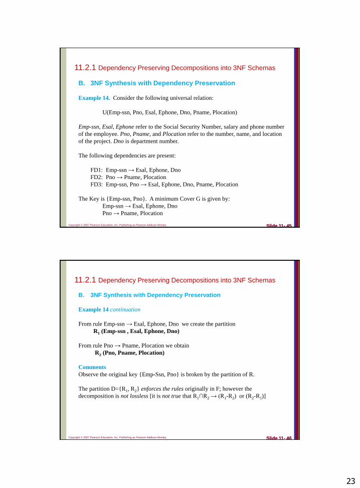
Example 14. Consider the following universal relation:

U(Emp-ssn, Pno, Esal, Ephone, Dno, Pname, Plocation)

Emp-ssn, Esal, Ephone refer to the Social Security Number, salary and phone number

of the employee. Pno, Pname, and Plocation refer to the number, name, and location

of the project. Dno is department number.

The following dependencies are present:

FD1: Emp-ssn → Esal, Ephone, Dno

FD2: Pno → Pname, Plocation

FD3: Emp-ssn, Pno → Esal, Ephone, Dno, Pname, Plocation

The Key is {Emp-ssn, Pno}. A minimum Cover G is given by:

Emp-ssn → Esal, Ephone, Dno

Pno → Pname, Plocation




Example 14 continuation

From rule Emp-ssn → Esal, Ephone, Dno we create the partition

R1 (Emp-ssn , Esal, Ephone, Dno)

From rule Pno → Pname, Plocation we obtain

R2 (Pno, Pname, Plocation)

Comments

Observe the original key {Emp-Ssn, Pno} is broken by the partition of R.

The partition D={R1, R2} enforces the rules originally in F; however the

decomposition is not lossless [it is not true that R1∩R2 → (R1-R2) or (R2-R1)]

24




Example 15.

Consider r(ABCDEF) subject to the following FDs

F = { A→BCE, B → DE, ABD → CF. AC → DE )

Find a 3NF database for r under F.

Solution: Find a canonical cover for (r, F).

1. After Left Reduction:

Rule ABD → CF becomes A → CF

Rule AC → DE becomes A → DE

F= { A → BCE, B → DE, A → CF, A → DE)

2. After Right Reduction (not really necessary! – use projectivity instead)

Rule A → BCE becomes A → B

Rule A → DE becomes A → E

F= { A → B, B → DE, A → CF, A → E )

3. After Removing Redundant Rule(s):

Rule A → E is redundant (Trans. on A → B, B → E )

F= { A → B, B → DE, A → CF } after compacting similar left-hand-side rules

F= { A → BCF, B → DE )

Final Partition D = ( ABCF, BDE ) (clearly in 3NF format)


The following method –which includes a minor modification to Algorithm 11.2-

produces a decomposition D of R that does the following:

• Preserves dependencies

• Has the nonadditive join property

Algorithm 11.4. Relational Synthesis into 3NF with Dependency

Preservation and Nonadditive Join Property

Input: A universal relation R and a set of functional dependencies F on the

attributes of R.

1. Find a minimal cover G for F.

2. For each left-hand-side X of a functional dependency that appears in G create a relation schema in D with attributes {X {A1} {A2} . . . {Ak} }, where

X → A1, X → A2, . . . , X → Ak are the only dependencies in G with X as

left-hand-side (X is the key of this relation).

3. If none of the relation schemas in D contains a key of R, then create one more

relation schema in D that contains attributes that form a key of R.

4. Eliminate redundant relations from the resulting set of relations in the relational

database schema. A relation R is considered redundant if R is a projection of

another relation S in the schema; alternately, R is subsumed by S.

11.2.3 Dependency-Preserving and Nonadditive (Lossless) Join

Decomposition into 3NF Schemas

25


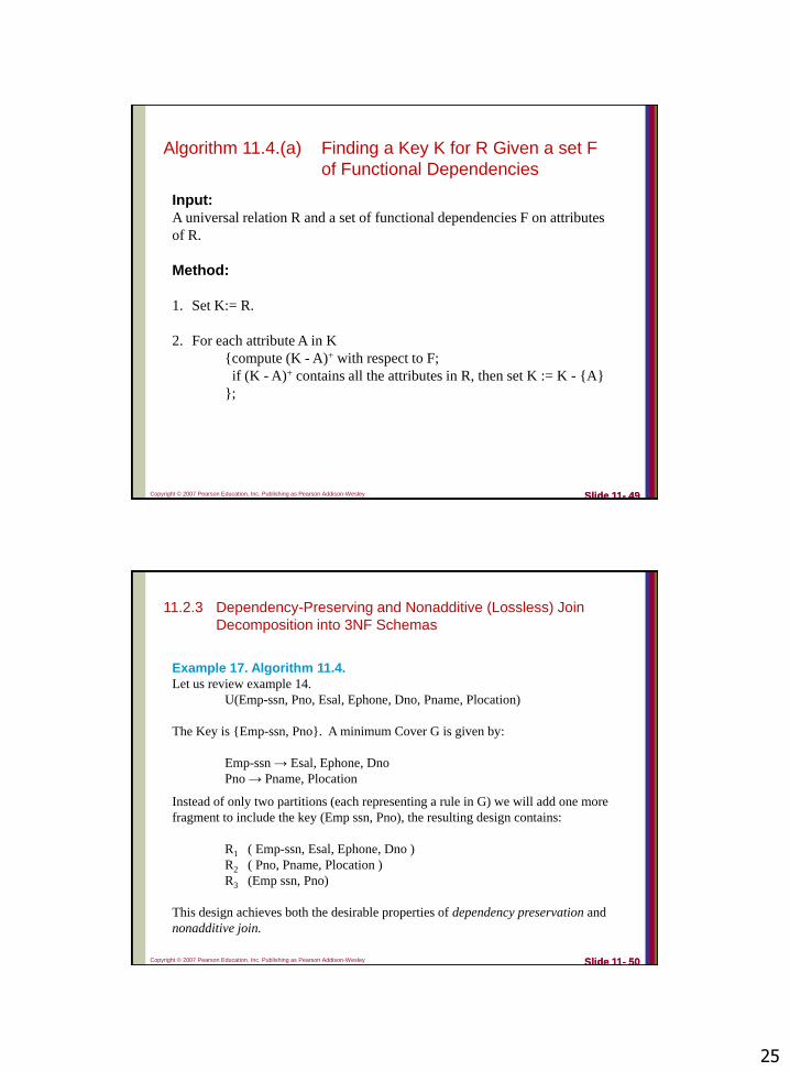
Algorithm 11.4.(a) Finding a Key K for R Given a set F

of Functional Dependencies

Input:

A universal relation R and a set of functional dependencies F on attributes

of R.

Method:

1. Set K:= R.

2. For each attribute A in K

{compute (K - A)+ with respect to F;

if (K - A)+ contains all the attributes in R, then set K := K - {A}

};


Example 17. Algorithm 11.4.

Let us review example 14.

U(Emp-ssn, Pno, Esal, Ephone, Dno, Pname, Plocation)

The Key is {Emp-ssn, Pno}. A minimum Cover G is given by:

Emp-ssn → Esal, Ephone, Dno

Pno → Pname, Plocation

Instead of only two partitions (each representing a rule in G) we will add one more

fragment to include the key (Emp ssn, Pno), the resulting design contains:

R1 ( Emp-ssn, Esal, Ephone, Dno )

R2 ( Pno, Pname, Plocation )

R3 (Emp ssn, Pno)

This design achieves both the desirable properties of dependency preservation and

nonadditive join.



26


Example 18. Algorithm 11.4.

Consider the relation LOTS1 and its

functional dependencies F.

F = { P→LCA, LC →AP, A →C }

A minimum cover G is

{P → LC, LC → AP, A → C }.

In step 2 of Algorithm 11.4 we produce design X (before removing redundant relations)

as

Design X: R1 (P, L, C), R2 (L, C, A, P), and R3 (A, C).

In step 4 of the algorithm, we find that R3 and R1 are subsumed by R2. Hence both of

those relations are redundant. Thus the 3NF schema that achieves both of the desirable

properties

is (after removing redundant relations)

Design X: R2 (L, C, A, P).



Copyright © 2007 Pearson Education, Inc. Publishing as Pearson Addison-Wesley

Slide 11- 52

11.2. Summary of Relational Database Design Algorithms

Slide 11- 52

27


Introduction. Functional Dependencies are not capable of representing all type of

associations between attributes.

In general a FD X→Y represents a many:1 relationship.

Sometimes we want to emphasize a many:many association or multiple 1:many

relationships in the same table.

In this case multivalued dependencies might be more appropriated.

11.3 Multivalued Dependencies and Fourth Normal Form (4NF)

Book# Author Price

B1 A1 100

B1 A2 100

B1 A3 100

B2 A4 90

B3 A1 120

B3 A5 120

Book# Author Price

B1 { A1, A2, A3 } 100

B2 { A4 } 90

B3 { A1, A5 } 120

NFNF 1:many Book : Author

Equivalent 1NF

relation

Book


Example 19. • Multiple independent 1:many relationships in the same table.

• Observe that ProjectName and DependentName are independent.


Ename Pname DependentName

Smith Proj-X Johnny

Smith Proj-Y Anna

Smith Proj-X Anna

Smith Proj-Y Johnny

Ename Pname

Smith Proj-X

Smith Proj-Y

Ename DependentName

Smith Johnny

Smith Anna

28


DefinitionA multivalued dependency XY specified on relation schema R, where X and Y are

both subsets of R, specifies the following constraint on any relation state r of R:

If two tuples t1 and t2 exist in r such that t1[X] = t2[X], then two tuples t3 and t4

should also exist in r with the following properties

t3[X] = t4[X] = t1[X] = t2[X].

t3[Y] = t1[Y] and t4[Y] = t2[Y].

t3[Z] = t2[Z] and t4[Z] = t1[Z] [we use Z to denote (R - (X Y)) ].

Whenever X Y holds, we say that X multi-determines Y.

Because of the symmetry in the definition, whenever XY holds in R, so does

X Z. Hence, XY implies XZ, and therefore it is sometimes written as X Y |

Z.



Example 20.aConsider the tuples t1, t2, t3, and t4 shown below. Observe that

t3[X] = t4[X] = t1[X] = t2[X].

t3[Y] = t1[Y] and t4[Y] = t2[Y].

t3[Z] = t2[Z] and t4[Z] = t1[Z]

Therefore XY and XZ i.e. Ename Pname , Ename DependentName


X Y Z


t1 Smith Proj-X Johnny

t2 Smith Proj-Y Anna

t3 Smith Proj-X Anna

t4 Smith Proj-Y Johnny

t3[X] = t4[X] = t1[X] = t2[X] = “Smith”

t3[Y] = t1[Y] = „Proj-X‟

t4[Y] = t2[Y] = „Proj-Y‟

t3[Z] = t2[Z] = „Anna‟

t4[Z] = t1[Z] = „Johnny‟

29


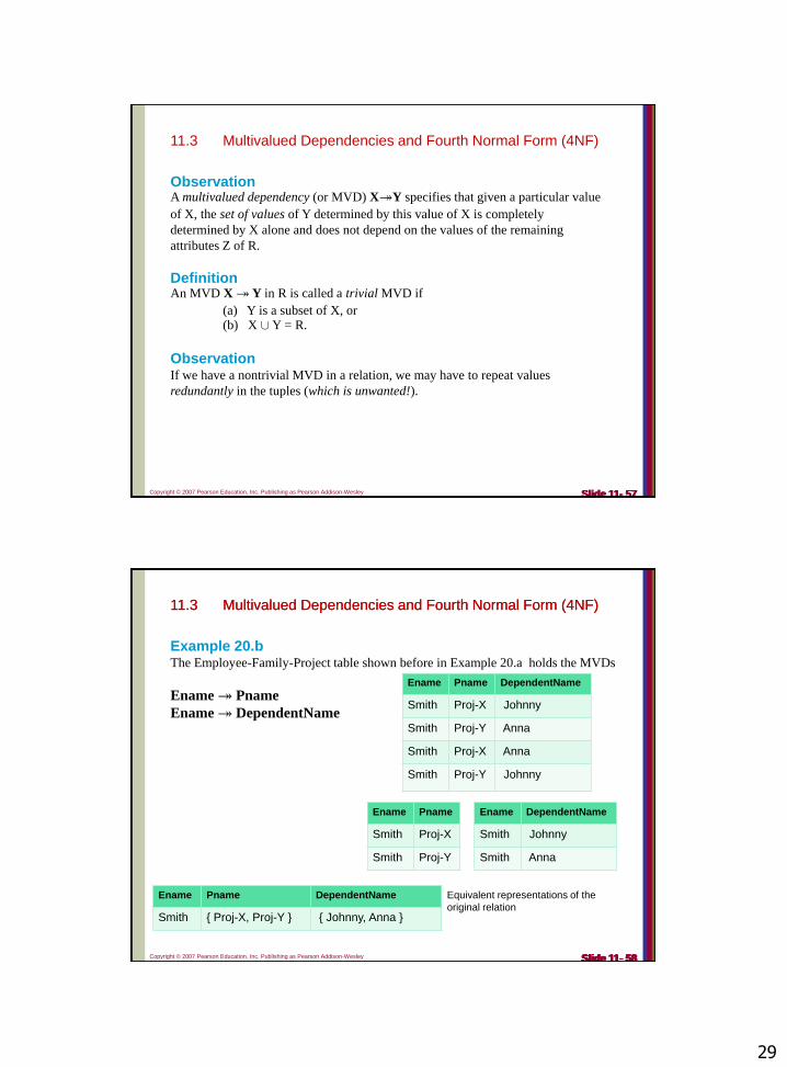
ObservationA multivalued dependency (or MVD) XY specifies that given a particular value

of X, the set of values of Y determined by this value of X is completely

determined by X alone and does not depend on the values of the remaining

attributes Z of R.

DefinitionAn MVD XY in R is called a trivial MVD if

(a) Y is a subset of X, or(b) X Y = R.

ObservationIf we have a nontrivial MVD in a relation, we may have to repeat values

redundantly in the tuples (which is unwanted!).




Slide 11- 58Slide 11- 58Slide 11- 58

Example 20.bThe Employee-Family-Project table shown before in Example 20.a holds the MVDs

Ename Pname

Ename DependentName



Smith Proj-X Johnny

Smith Proj-Y Anna

Smith Proj-X Anna

Smith Proj-Y Johnny

Ename Pname

Smith Proj-X

Smith Proj-Y

Ename DependentName

Smith Johnny

Smith Anna


Smith { Proj-X, Proj-Y } { Johnny, Anna }

Equivalent representations of the

original relation

30


Inference rules for Multivalued DependenciesThe following inference rules IR1 through IR8 form a sound and complete set for

inferring functional and multivalued dependencies from a given set of dependencies.

Assume that all attributes are included in a universal relation schema

R = {A1, A2, . . . ,Am} and that X, Y, Z, and W are subsets of R.

IR1 (reflexive rule for FDs): If X Y, then X→Y.

IR2 (augmentation rule for FDs): {X → Y} XZ → YZ.

IR3 (transitive rule for FDs): {X → Y, Y → Z} X → Z.

IR4 (complementation rule for MVDs): {X Y) {X (R - ( X Y))}:

IR5 (augmentation rule for MVDs): If X Y and W Z, then WX YZ.

IR6 (transitive rule for MVDs): {X Y, Y Z} X (Z - Y).

IR7 (replication rule for FD to MVD): {X → Y) X Y.

IR8 (coalescence rule for FDs and MVDs): If XY and there exists W with the

properties that (a) W ∩ Y is empty, (b) W → Z, and (c) Y Z, then X → Z.

IR9 (Additivity) If XY and X Z then X YZ

IR10(Projectivity) If X Y and X Z, then X Y∩Z, X Y - Z, and X Z – Y

Note: IR9 and IR10 are derived from IR1-IR8. See D. Maier Chp 7 pp 129



How to know if a given m.v.d.

holds in a relation r ?

Is ABC valid in r ?

Method

1. Decompose r into r1(ABC) and r2(ADE)

2. Join r1 and r2 (call it r12)

3. Compare r with r12

if both are equal the depenency holds.


r A B C D Ea1 b1 c1 d1 e1a2 b3 c3 d3 e3a2 b3 c3 d4 e4a2 b3 c3 d3 e4a2 b3 c3 d4 e3a3 b4 c4 d5 e5a3 b4 c4 d5 e6a3 b4 c4 d6 e5a3 b4 c4 d6 e6a3 b5 c5 d5 e5a3 b5 c5 d5 e6a3 b5 c5 d6 e5a3 b5 c5 d6 e6

A D Ea1 d1 e1a2 d3 e3a2 d3 e4a2 d4 e3a2 d4 e4a3 d5 e5a3 d5 e6a3 d6 e5a3 d6 e6

A B C

a1 b1 c1

a2 b3 c3

a3 b4 c4

a3 b5 c5

r1 r2

1. In this example ABC

is valid.

2. Your turntry BC CD

31


How to know if a given m.v.d.

holds in a relation r ?

Testing validity of BCCD

Method

1. Decompose r into r1(BCD) and r2(ABDE)

2. Join r1 and r2 (call it r12)

3. Compare r with r12

if both are equal the dependency holds.


r A B C D Ea1 b1 c1 d1 e1a2 b3 c3 d3 e3a2 b3 c3 d4 e4a2 b3 c3 d3 e4a2 b3 c3 d4 e3a3 b4 c4 d5 e5a3 b4 c4 d5 e6a3 b4 c4 d6 e5a3 b4 c4 d6 e6a3 b5 c5 d5 e5a3 b5 c5 d5 e6a3 b5 c5 d6 e5a3 b5 c5 d6 e6

r1r2

In this example BCBD

is valid.

B C D

b1 c1 d1

b3 c3 d3

b3 c3 d4

b4 c4 d5

b4 c4 d6

b5 c5 d5

b5 c5 d6

A B D Ea1 b1 d1 e1a2 b3 d3 e3a2 b3 d3 e4a2 b3 d4 e3a2 b3 d4 e4a3 b4 d5 e5a3 b4 d5 e6a3 b4 d6 e5a3 b4 d6 e6a3 b5 d5 e5a3 b5 d5 e6

a3 b5 d6 e5a3 b5 d6 e6


Inference rules for Multivalued Dependencies

MVD Transitivity

Rule IR6 (transitive rule for MVDs): {X Y, Y Z} X (Z – Y)

Example

ABC

BC CD

A D (i.e. CD – BC)

Observe that

a1 {b1c1} {d1}

a2 {b3c3} {d3,d4}

a3{b4c4, b5c5} {d5, d6}


A B C D E

a1 b1 c1 d1 e1

a2 b3 c3 d3 e3

a2 b3 c3 d4 e4

a2 b3 c3 d3 e4

a2 b3 c3 d4 e3

a3 b4 c4 d5 e5

a3 b4 c4 d5 e6

a3 b4 c4 d6 e5

a3 b4 c4 d6 e6

a3 b5 c5 d5 e5

a3 b5 c5 d5 e6

a3 b5 c5 d6 e5

a3 b5 c5 d6 e6

32


Inference rules for Multivalued Dependencies

MVD CoalescenseIR8 (coalescence rule for FDs and MVDs): If XY and there exists W with

the properties that

(a) W ∩ Y is empty,

(b) W → Z, and (c) Y Z,

then X → Z.

Example

S Day Hour ChannelS SponsorS Actor

TVstation → Channel

S → Channel


Show Day Hour Channel Tvstation Sponsor Actor

s1 Mo 9p 1 ABC Nike Angeline

s1 Mo 9p 1 ABC Nike Sandra

s1 Mo 9p 1 ABC Pepsi Angeline

s1 Mo 9p 1 ABC Pepsi Sandra

s2 We 8p 3 CBS ATT Fox

s2 We 8p 3 CBS ATT Scully

s2 We 8p 3 CBS IBM Fox

s2 We 8p 3 CBS IBM Scully

s3 Tu 7p 1 ABC Toyota Columbus

s3 Fr 7p 1 ABC Toyota Columbus


Example 21A. Inference rules for Multivalued Dependencies

Consider the dependencies F = { A BC, DE C} over the schema

R = {ABCDE}.

QuestionDoes AD BE ?

Proof. Using the Inference Axioms IR1 to IR8 we have1. ABC given

2. A DE by complementation respect to R

3. DEC given

4. AC transitivity on 2 and 3

5. AD C augmentation of 4 by D

6. AD BE complementation of 5 respect to R


33


Example 21B. Inference rules for Multivalued Dependencies

Consider the dependencies F = { AEI, C AB } on the schema

R = { ABCDEI }.

QuestionDoes AC BEI ?

Proof. Using the Inference Axioms IR1 to IR8 we have1. CAB given

2. C DEI complementation of 1 respect to R

3. CEIDEI augmentation of 2 by EI

4. A EI given

5. AC CEI augmentation of 4 by C

6. AC D transitivty on 5 and 3

7. AC BEI complementation of 5 respect to R



Example 21C. Inference rules for Multivalued Dependencies

Consider the dependencies F = { AEI, C AB } on the schema

R = { ABCDEI }.

QuestionDoes AC B ?

Proof. Using the Inference Axioms IR1 to IR8 we have1. CAB given

2. C DEI complementation of 1 respect to R

3. AC ADEI augmentation of 3 by A

4. ACB complementation of 3 respect to R


34

Copyright © 2007 Pearson Education, Inc. Publishing as Pearson Addison-Wesley Slide 11- 67Slide 11- 67Slide 11- 67Slide 11- 67Slide 11- 67Slide 11- 67

Minimal Disjoint Set Basis

Definition: Given a collection of sets S = {S1, S2, … SP}, where the universe U = S1 S2

… SP the minimal disjoint set basis of S (mdsb(S)) is the partition T= {T1,

T2, …Tq} of U such that

1. Every Si is a union of some of the Tj‟s

2. No partition of U with fewer cells has the first property

Example

Assume S = {ABC, BCD, AD } then mdsb(S) = { A, BC, D }

Observe that ABC = A + BC

BCD = BC + D

AD = A + D


Copyright © 2007 Pearson Education, Inc. Publishing as Pearson Addison-Wesley Slide 11- 68Slide 11- 68Slide 11- 68Slide 11- 68Slide 11- 68Slide 11- 68

Algorithm. Computing Dependency Basis Input:

A set of multivalued dependencies M over a set of attributes R, and a set X U

Output: The dependency basis for X with respect to M.

Method: 1. Let T be the set of sets Z X such that for some WY in M, we have WX,

and Z is either (Y – X) or ( R – X – Y )

2. Until T consists of a disjoint collection of sets, find a pair of sets Z1 and Z2 in T that are not disjoint and replace them by sets (Z1 - Z2), (Z2 – Z1) and (Z1 Z2).

Let S be the final collection of sets.

3. Until no more changes can be made to S, look for dependencies VW in M and

a set Y in S such that Y intersects W but not V. Replace Y by the sets ( Y W)

and ( Y – W ) in S.

4. The final collection of sets in S is the dependency basis for X.


35

Copyright © 2007 Pearson Education, Inc. Publishing as Pearson Addison-Wesley Slide 11- 69Slide 11- 69Slide 11- 69Slide 11- 69Slide 11- 69Slide 11- 69Slide 11- 69

Algorithm. Computing Dependency Basis

IntuitionAssume we are computing DEP(AC) for schema R under M(Functional and Multivalued ). STEP1 begins with the application of reflexivity AC AC and

complementation AC R-AC. Therefore the initial set TAC includes {A, R-A}.

Exploring rules in M of the form AC X1, A X2 and C X3 brings to TAC

other attributes directly implied by AC. Observe that by augmentation if A X2

then AC X2, similarly if C X3 by augmentation AC X3. Therefore fragments

X1, X2, X3 (and their complements) must also be added to TAC.

If no more elements can be included to TAB a fine fragmentation of the existing TAB

components should follow to produce its mdsb(TAC) (called SAC in the algorithm).

In the final step, we try one more refinement of the elements Y in SAC = msdb(TAC). The Coalescence axiom (IR8) states that if there is a dependency VW in M and a

set Y in SAC such that Y intersects W but not V then AC W. Therefore the set Y

could be replaced by the finer sets ( Y W) and ( Y – W ) in SAC.

The final collection of sets in SAC is the dependency basis DEP(AC).



ClaimTo test whether a MVD X Y holds in F, it suffices to determine DEP(X)

and see whether (Y - X) is the union of some sets in DEP(X).

Example 22ALet F={A BC, DE C} be a set of MVDs over ABCDE.

Compute DEP(A)To compute it we begin with TA = {A, BCDE} (AA, A BCDE).

Step 1 allows us to use A BC (given) and introduce BC in TA.

Observe that A DE (by use of complementation), therefore DE is also

added to TA = {A, BCDE, BC, DE}.

Refining this set produces SA = {A, BC, DE}. Using Step3 of the method we find rule DE C and element BC intersects

the RHS; however BC does not share common attributes with DE (the LHS). Consequently we replace BC with (BC C) and (BC – C).

Hence DEP(A)={A, B, C, DE}


36


Example 22A continuation

Let F={A BC, DE C} be a set of MVDs over ABCDE.

Hence DEP(A)={A, B, C, DE}

Significance

Attribute A multi-determines any union of elements in DEP(A), for

example

AA A BC

AB ADE

AC ACDE

ABCDE

ABDE

Similarly we may say it is NOT true that A D [notice D is not an element

of DEP(A) ]



Example 22A continuation

Let F={A BC, DE C} be a set of MVDs over ABCDE.

In a similar way DEP(AD) = { A, B, C, D, E }

DEP(BC) = { B, C, ADE } and so on…

Why?

Let us compute the dependency basis of AD. We begin with a set TAD consisting

of {AD, BCE}. Then we look for MVDs whose LHS is in AD, such as A B, A C, AA (see first part of this problem)

Therefore TAD = { AD, BCE, A, B, C, BCDE, CDE, BDE, DE, BC }

Refining of this set produces SAD = {A, B, C, D, E } = DEP(AD)

Similarly, computing DEP( BC ) begins with TBC = {BC, ADE} = SBC

Nothing else can be added to TBC. Now consider Y=BC and the rule DE C.

The RHS of this rule and Y intersect but its LHS has nothing in common with

BC. Step3 of the DEP _BASIS algorithm tells us to replace BC with (BC∩C) and

(BC - C). That is, C and B. Therefore DEP( BC) = {B, C, ADE}.


37


Example 22BLet F = { AEI, C AB } be a set of MVDs over ABCDEI.

Find DEP(AC). See problems 21B and 21C

DEP(AC) = { A, B, C, D, EI }

Why?

Let us compute the dependency basis of AC.

We begin with a set TAC consisting of {AC, BDEI}. Then we look for MVDs whose LHS is in AD, such as A EI, A BCD, CAB, C DEI.

Therefore TAC = { AC, BDEI, EI, BCD, AB, DEI }

Refining of this set produces SAC = {A, B, C, D, EI }.

In problem 21B we were asked to show that AC BEI. Observe that B and EI

are elements in DEP(AC) therefore ACBEI, similarly AC B (see problem

21C) .



Example 22C. (from J. Ullman – Database Systems)

Consider the following relation

R= (Course, Teacher, Hour, Room, Student, Grade)

By observation we find the following MVDs

C HR C SG

C →T HT →R

HR →C CS →G

HS →R

Notice that DEP(C) = { T, SG, HR }.

Therefore C T, C HR, C THR, C TSG, C HRSG, C THRSG,

Also observe that the MVD C R is invalid (Room and Hour are depend on each other)

Other example is DEP(HR) = {HR, TSG} from here we conclude it is not true that HR SG


38


Definition. Nonadditive Join Decomposition into 4NF Relations

Whenever we decompose a relation schema R into R1 = (X Y) and R2 = (R - Y)

based on an MVD X Y that holds in R, the decomposition has the nonadditive

join property.

Property NJB. The relation schemas R1 and R2 form a non-additive join

decomposition of R with respect to a set F of functional and multivalued

dependencies if and only if

R1 ∩ R2 (R1 – R2) or

R1 ∩ R2 (R2 – R1)

Example:

The relation Book(Book#, Author, Price) with multivalued dependencies F= { Book#Author, Book# → Price } has a lossless decomposition in

R1 = (Book#, Author)

R2 = (Book#, Price)



Definition Fourth Normal Form (4NF)Fourth normal form (4NF) schema is violated when a relation has

undesirable non-trivial multivalued dependencies (it should be decomposed)

Definition.

A relation schema R is in 4NF with respect to a set of dependencies F (that

includes functional dependencies and multivalued dependencies) if, for every nontrivial multivalued dependency XY in F+, X is a superkey for R.

Observation.In the previous definition the determination of superkey values is solely

based on functional dependencies in F.


39

Copyright © 2007 Pearson Education, Inc. Publishing as Pearson Addison-Wesley Slide 11- 77Slide 11- 77Slide 11- 77Slide 11- 77

Algorithm 11.5. Relational Decomposition into 4NF

Relations with Nonadditive Join PropertyInput:

A universal relation R and a set of functional and multivalued dependencies

F.

Method

1. Set D:= { R }

2. While there is a relation schema Q in D that is not in 4NF, do

{ choose a relation schema Q in D that is not in 4NF;find a nontrivial MVD X Y in Q that violates 4NF;

replace Q in D by two relation schemas (Q - Y) and (XY);

}



Example 23.Consider the previous example where R= {CTHRSG} and the dependencies are F = { C HR, C SG, C → T }.

1. Observe that MVDs in F are not trivial and C is NOT a superkey in R.

2. Therefore we could use the rule C HR to decompose the table into

fragments: {R1=CHR, R2=CSGT}. The mvd C HR in R1 becomes trivial.

3. Again, C is not a superkey in R2 and the MVD C SG is not trivial

4. Therefore we could partition R2 into R21=CSG, R22=CT where R21 holds a

trivial MVD, and R22 has only one rule C → T in which C is a superkey.

5. The final 4NF Lossless database schema is D = { CHR, CSG, CT }


40


Definition. Join Dependencies

A join dependency (JD), denoted by JD(R1, R2, . . . , Rn), on relation schema R,

specifies a constraint on the states r of R. The constraint requests that every legal

state r of R should have a non-additive join decomposition into R1, R2, . . . , Rn

That is, for every such r we have

* ( R1(r), R2(r), …, Rn(r) ) = r

Notice that an MVD is a special case of a JD where n = 2. That is, a JD denoted as JD(R1, R2) implies an MVD (R1 ∩ R2) (R1 – R2) (or (R2 – R1) ).

Definition

A join dependency JD(R1, R2, . . . , Rn), specified on relation schema R, is

a trivial JD if one of the relation schemas Ri in JD(R1, R2, . . . , Rn) is equal to R.

11.4 Join Dependencies and Fifth Normal Form (5NF)


Definition. Fifth Normal Form (5NF) or Projection-Join NF (PJNF)

A relation schema R is in fifth normal form (5NF) with respect to a set F of

functional, multivalued, and join dependencies if, for every nontrivial join

dependency JD(R1, R2, . . . , Rn), in F+ every Ri is a superkey of R.

ObservationFifth normal form deals with cases where information can be reconstructed from

smaller pieces of information that can be maintained with less redundancy. The

big difficulty of reaching 5NF is that all possible decompositions of R must

support the lossless join property.

Note: Discovering JDs in practical databases with hundreds of attributes is next to impossible.

Therefore, the current practice of database design pays little attention to them.


41


Example 24. Fifth Normal Form (5NF) or Projection-Join NF (PJNF)


5NF demands that all possible projections of r(R) on a given decomposition DR ,

losslessly regenerate the original table. Consider a decomposition of the example

schema R= (Agent, Company, Product) into the following two sub-schemas:

R1(Agent, Company) and R2(Company, Product)

Using the given data is easy to proof that R1(r) * R2(r) r

(phantom tuples such as <Brown, GM, truck>

will be produced) . Hence R is not in 5NF.

However r(R) has a 5NF representation using

the three trivial schemas: R1, R2, R3 given below.


Observation

Inclusion dependencies were defined in order to formalize two types of

inter- relational constraints that cannot be represented with FD/MVD/JDs:

• Foreign key (or referential integrity) relates attributes across relations.

• Inheritance represent a class/subclass relationship.

Definition.

An inclusion dependency R.X < S.Y between two sets of attributes-X of

relation schema R, and Y of relation schema S-specifies the constraint that,

at any specific time when r is a relation state of R and s a relation state of S,

we must have

X(s(S)) Y(r(R))

11. 5 Inclusion Dependencies

42



Example 25we can specify the following (referential

Integrity type) inclusion dependencies

on the relational schema in Figure 10.1



Example 26we can specify the following (inheritance type) inclusion dependencies on the

relational schema in Figure 7.1

43


DefinitionAs with other types of dependencies, there are inclusion dependency inference rules

(IDIRs). The following are three examples:

IDIR1 (reflexivity): R.X < R.X.

IDIR2 (attribute correspondence): If R.X < S.Y, where X = {A1, A2, . . . ,An}

and Y = {B1, B2, . . . , Bn} and Ai Corresponds to Bi

then R.Ai < S.Bi for 1i n.

IDIR3 (transitivity): If R.X < S.Y and S.Y < T.Z, then R.X < T.Z.

The preceding inference rules were shown to be sound and complete for inclusion

dependencies. So far, no normal forms have been developed based on inclusion

dependencies.



RationaleTemplate dependencies provide a technique for representing constraints in relations

that typically have no easy and formal definitions.

The idea behind template dependencies is to specify a template-or example-that

defines each constraint or dependency.

There are two types of templates: tuple-generating templates and constraint

generating templates.

• A template consists of a number of hypothesis tuples that are meant to show an

example of the tuples that may appear in one or more relations.

• The other part of the template is the template-conclusion. the conclusion is a set

of tuples that must also exist in the relations if the hypothesis tuples are there.

• For constraint-generating templates, the template conclusion is a condition that

must hold on the hypothesis tuples.

11. 6 Template Dependencies

44





45


Functional Dependencies Based on Arithmetic

Functions and Procedures

Sometimes the attributes in a relation may be related via some arithmetic function

or a more complicated functional relationship. As long as a unique value of Y is

associated with every X, we can still consider that the FD X →Y exists. For

example, in the relationORDER-LINE (Order#, Item#, Quantity, Unit-price, Extended-price, Discounted-price)

In this relation,

(Quantity, Unit-price ) → Extended-price

by the formula

Extended-price = Unit-price * Quantity.

Although the above kinds of FDs are technically present in most relations, they are

not given particular attention during normalization.



References

David Maier, "The Theory of Relational Databases", Comp. Sc. Press, 1983.

Desai, Bipin, An Introduction to Database Systems, West Publishing, 1990

Ullman, J. Principles of Database Systems. Computer Science Press, 1982.

H. Mannila, K. Raiha, “The Design of Relational Databases”. Addison-Wesley, 1992.

Elmasri, Navathe, “Fundamentals of Database Systems”, 5th Ed. Addisson-Wesley, 2007.

Silberschatz, Korth, Surdarshan, “Database System Concepts”, McGraw-Hill, 2011

William Kent, "A Simple Guide to Five Normal Forms in Relational Database Theory",

Communications of the ACM 26(2), Feb. 1983

Questions ?

chapter 11 - cleveland state universitycis.csuohio.edu/~sschung/cis611/enach11-further...successive...

Documents