chapter 11 classiﬁcation algorithms and regression trees · chapter 11 classiﬁcation algorithms...

Chapter 11

Classification Algorithms andRegression Trees

The next four paragraphs are from the book by Breiman et. al.

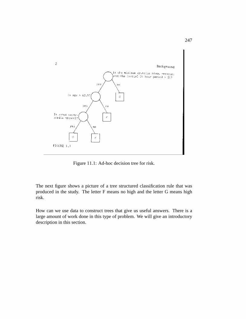
At the university of California, San Diego Medical Center, when a heart attackpatient is admitted, 19 variables are measured during the first 24 hours. They in-clude BP, age and 17 other binary covariates summarizing the medical symptomsconsidered as important indicators of the patient’s condition.

The goal of a medical study can be to develop a method to identify high riskpatients on the basis of the initial 24-hour data.

246

247

Figure 11.1: Ad-hoc decision tree for risk.

The next figure shows a picture of a tree structured classification rule that wasproduced in the study. The letter F means no high and the letter G means highrisk.

How can we use data to construct trees that give us useful answers. There is alarge amount of work done in this type of problem. We will give an introductorydescription in this section.

248CHAPTER 11. CLASSIFICATION ALGORITHMS AND REGRESSION TREES

The material here is based on lectures by Ingo Ruczinski.

11.1 Classifiers as Partitions

Notice that in the example above we predict a positive outcome if both blood pres-sure is highand age is higher than 62.5. This type of interaction is hard to describeby a regression model. If you go back and look at the methods we presented youwill notice that we rarely include interaction terms mainly because of the curse ofdimensionality. There are too many interactions to consider and too many ways toquantify their effect. Regression trees thrive on such interactions. What is a cursefor parametric and smoothing approaches is a blessing for regression trees.

A good example is the following olive data:

• 572 olive oils were analyzed for their content of eight fatty acids (palmitic,palmitoleic, stearic, oleic, linoleic, arachidic, linolenic, and eicosenoic).

• There were 9 collection areas, 4 from Southern Italy (North and South Apu-lia, Calabria, Sicily), two from Sardinia (Inland and Coastal) and 3 fromNorthern Italy (Umbria, East and West Liguria).

• The concentrations of different fatty acids vary from up to 85% for oleicacid to as low as 0.01% for eicosenoic acid.

• See Forina M, Armanino C, Lanteri S, and Tiscornia E (1983).Classifi-cation of olive oils from their fatty acid composition. In Martens H and

11.1. CLASSIFIERS AS PARTITIONS 249

Figure 11.2: Olive data.

Russwurm Jr H, editors, Food Research and Data Analysis, pp 189-214.Applied Science Publishers, London.

The data look like this:

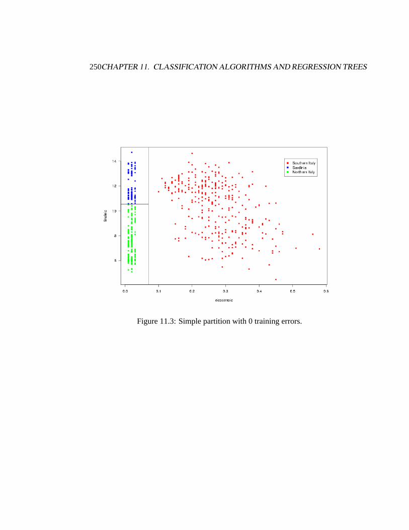
Notice that we can separate the covariate space so that we get perfect predictionwithout a very complicated “model”.


Figure 11.3: Simple partition with 0 training errors.


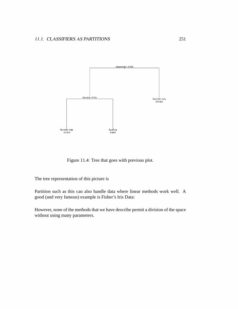
Figure 11.4: Tree that goes with previous plot.

The tree representation of this picture is

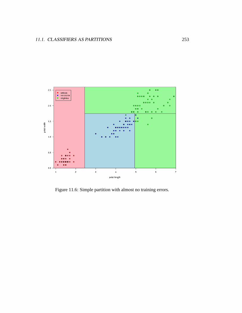
Partition such as this can also handle data where linear methods work well. Agood (and very famous) example is Fisher’s Iris Data:

However, none of the methods that we have describe permit a division of the spacewithout using many parameters.


Figure 11.5: Iris Data.


Figure 11.6: Simple partition with almost no training errors.


Figure 11.7: Tree for the previous plot.

11.2. TREES 255

11.2 Trees

These data motivates the approach of partitioning the covariate spaceX into dis-joint setsA1, . . . , Aj with G = j for all x ∈ Aj. There are too many ways ofdoing so we ways to make the approach more parsimonious. Notice that linearregression restricts divisions to certain planes.

Trees are a completely different way of partitioning. All we require is that thepartition can be achieved by successive binary partitions based on the differentpredictors. Once we have a partition such as this we base our prediction on theaverage of theY s in each partition. We can use this for both classification andregression.

11.2.1 Example of classification tree

Suppose that we have a scalar outcome,Y , and ap-vector of explanatory variables,X. AssumeY ∈ K = {1, 2, . . . , k}


&%'$

&%'$

&%'$

&%'$

1 2 1

2 3

��

��

@@

@@@

��

��

��

AAAAAA

��

��

��

AAAAAA

��

��

��

AAAAAA

x1

x2 x3

x2

< 5 ≥ 5

> 3 ≤ 3 = 2 6= 2

> 1 ≤ 1

The subsets created by the splits are callednodes. The subsets which are not splitare called terminal nodes.

Each terminal nodes gets assigned to one of the classes. So if we had 3 classeswe could getA1 = X5 ∪ X9, A2 = X6 andA3 = X7 ∪ X8. If we are using thedata we assign the class most frequently found in that subset ofX . We call these

11.2. TREES 257

classification tress.

A classification tree partitions theX-space and provides a predicted value, per-haps arg maxs Pr(Y = s|X ∈ Ak) in each region.

11.2.2 Example of regression tree

Again, suppose that we have a scalar outcome,Y , and ap-vector of explanatoryvariables,X. Now assumeY ∈ R.


&%'$

&%'$

&%'$

&%'$

13 34 77

51 26

��

��

@@

@@@

��

��

��

AAAAAA

��

��

��

AAAAAA

��

��

��

AAAAAA

x1

x2 x3

x2

< 5 ≥ 5

> 3 ≤ 3 = 2 6= 2

> 1 ≤ 1

A regression tree partitions theX-space into disjoint regionsAk and provides afitted value E(Y |X ∈ Ak) within each region.

11.2. TREES 259

Figure 11.8: Comparison of CART and Linear Regression

11.2.3 CART versus Linear Models

See Figure 11.8.


11.3 Searching for good trees

In general the idea the following:

1. Grow an overly large tree using forward selection. At each step, find thebestsplit. Grow until all terminal nodes either

(a) have< n (perhapsn = 1) data points,

(b) are “pure” (all points in a node have [almost] the same outcome).

2. Prune the tree back, creating a nested sequence of trees, decreasing in com-plexity.

A problem in tree construction is how to use the training data to determine thebinary splits ofX into smaller and smaller pieces. The fundamental idea is toselect each split of a subset so that the data in each of the descendant subsets are“purer” than the data in the parent subset.

11.3.1 The Predictor Space

Suppose that we havep explanatory variablesX1, . . . , Xp andn observations.

Each of theXi can be

11.3. SEARCHING FOR GOOD TREES 261

a) a numeric variable:−→ n− 1 possible splits.

b) an ordered factor:−→ k − 1 possible splits.

b) an unordered factor:−→ 2k−1 − 1 possible splits.

We pick the split that results in the greatest decrease inimpurity. We will soonprovide various definitions of impurity.

11.3.2 Deviance as a measure of impurity

A simple approach to classification problems is to assume a multinomial modeland then use deviance as a definition of impurity.

AssumeY ∈ G = {1, 2, . . . , k}.

• At each nodei of a classification tree we have a probability distributionpik

over thek classes.

• We observe a random samplenik from the multinomial distribution speci-fied by the probabilitiespik.

• GivenX, the conditional likelihood is then proportional to∏

(leavesi)

∏(classesk) pnik

ik .

• Define a devianceD =∑

Di , where Di = −2∑

k nik log(pik).

• Estimatepik by pik = nik

ni..


For the olive that we get the following values:

Root n11 = 246 n12 = 74 n13 = 116 n1 = 436 D = 851.2

p11 = 246436

p12 = 74436

p13 = 116436

Split 1 n11 = 246 n12 = 0 n13 = 0 n1 = 246 D = 254.0

n21 = 0 n22 = 74 n23 = 116 n2 = 190

p11 = 1 p12 = 0 p13 = 0

p21 = 0 p22 = 74190

p23 = 116190

Split 2 n11 = 246 n12 = 0 n13 = 0 n1 = 246 D = 0

n21 = 0 n22 = 74 n23 = 0 n2 = 74

n31 = 0 n32 = 0 n33 = 116 n3 = 116

11.3.3 Other measures of impurity

Other commonly used measures of impurity at a nodei in classification trees are

11.4. MODEL SELECTION 263

• the entropy:∑

pik log(pik).

• the GINI index:∑

j 6=k pijpik = 1−∑

k p2ik.

For regression trees we use the residual sum of squares:

D =∑

casesj

(yj − µ[j]

)2

whereµ[j] is the mean of the values in the node that casej belongs to.

11.3.4 Recursive Partitioning

INITIALIZE All cases in the root node.REPEAT Find optimal allowed split.

Partition leaf according to split.STOP Stop when pre-defined criterion is met.

11.4 Model Selection

• Grow a big treeT .

• Consider snipping off terminal subtrees (resulting in so-called rooted sub-trees).


• Let Ri be a measure of impurity at leafi in a tree. DefineR =∑

i Ri.

• Define size as the number of leaves in a tree.

• Let Rα = R + α× size.

The set of rooted subtrees ofT that minimizeRα is nested.

11.5 General Points

What’s nice:

• Decision trees are very “natural” constructs, in particular when the explana-tory variables are categorical (and even better, when they are binary).

• Trees are very easy to explain to non-statisticians.

• The models are invariant under transformations in the predictor space.

• Multi-factor response is easily dealt with.

• The treatment of missing values is more satisfactory than for most othermodel classes.

• The models go after interactions immediately, rather than as an afterthought.

• The tree growth is actually more efficient than I have described it.

11.6. CART REFERENCES 265

• There are extensions for survival and longitudinal data, and there is an ex-tension called treed models. There is even a Bayesian version of CART.

What’s not so nice:

• The tree-space is huge, so we may need a lot of data.

• We might not be able to find the “best” model at all.

• It can be hard to assess uncertainty in inference about trees.

• The results can be quite variable (the tree selection is not very stable).

• Actual additivity becomes a mess in a binary tree.

• Simple trees usually do not have a lot of predictive power.

• There is a selection bias for the splits.

11.6 CART References

• L Breiman.Statistical Modeling: The Two Cultures.Statistical Science, 16 (3), pp 199-215, 2001.

• L Breiman, JH Friedman, RA Olshen, and CJ Stone.Classification and Regression Trees.Wadsworth Inc, 1984.


• TM Therneau and EJ Atkinson.An Introduction to Recursive Partitioning Using the RPART Routines.Technical Report Series No 61, Department of Health Science Research,Mayo Clinic, Rochester, Minnesota, 2000.

• WN Venables and BD Ripley.Modern Applied Statistics with S.Springer NY, 4th edition, 2002.

11.7 Bagging

• Bagging predictors is a method for generating multiple versions of a predic-tor and using these to get an aggregated predictor.

• The aggregation averages over the versions when predicting a numericaloutcome and does a plurality vote when predicting a class.

• The multiple versions are formed by making bootstrap replicates of thelearning set and using these as new learning sets.

• The vital element is the instability of the prediction method. If perturbingthe learning set can cause significant changes in the predictor constructed,then bagging can improve accuracy.

Bagging =BootstrapAggregating

Reference: Breiman L (1996):Bagging Predictors, Machine Learning, Vol 24(2), pp 123-140.

11.7. BAGGING 267

Figure 11.9: Two bagging examples.

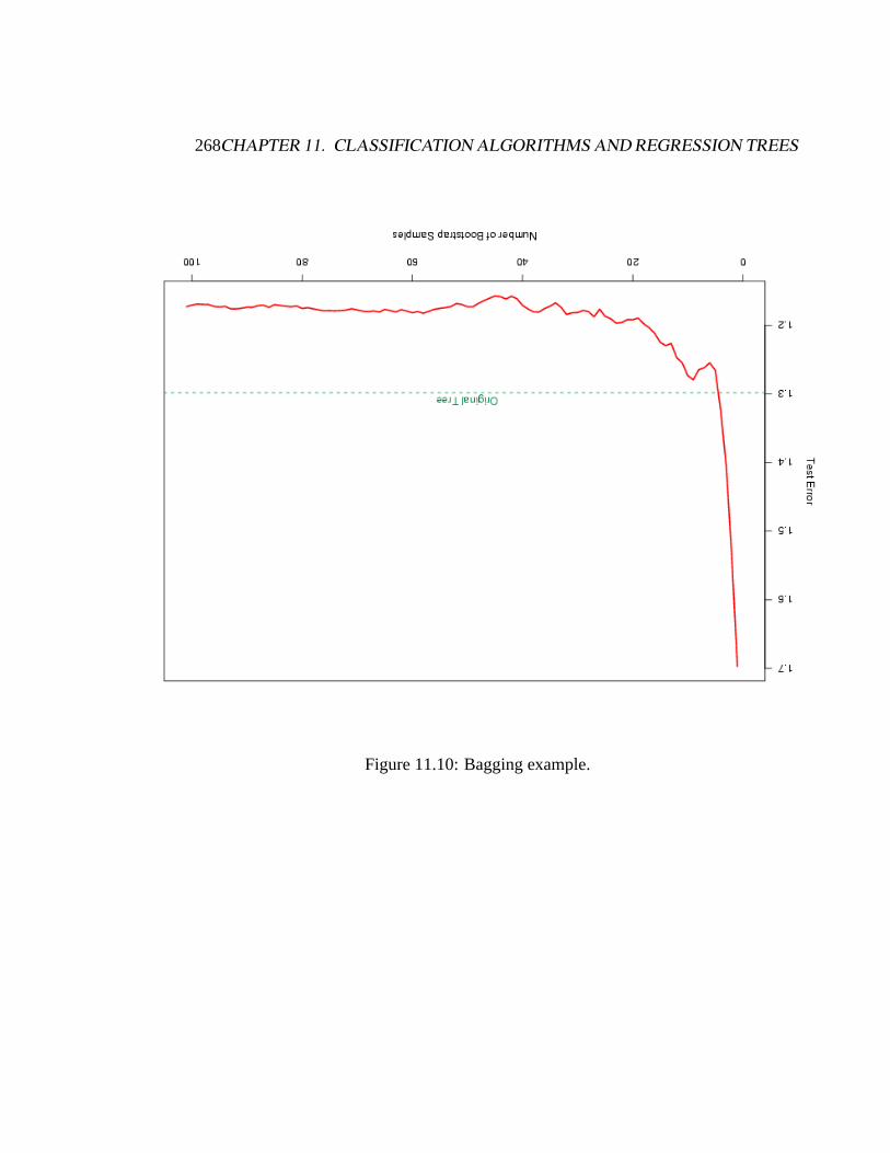
• Generate a sample of sizeN = 30 with two classes andp = 5 features, eachhaving a standard Gaussian distribution with pairwise correlation 0.95.

• The response was generated asY ∼ N(µ = 2− 4× I[X1>0.5] , σ2 = 1

)A test sample of size 2000 was also generated from the same population.

Note:

• Bagging can dramatically reduce the variance of unstable procedures suchas trees, leading to improved prediction.


Figure 11.10: Bagging example.

11.8. RANDOM FORESTS 269

• A simple argument can show why bagging helps under squared error loss:averaging reduces variance and leaves bias unchanged.

Reference: Hastie T, Tibshirani R, and Friedman J (2001):The Elements of Sta-tistical Learning, Springer, NY.

However:

• The above argument breaks down for classification under 0-1 loss.

• Other tree-based classifiers such as random split selection perform consis-tently better.

Reference: Dietterich T (2000):An Experimental Comparison of Three Methodsfor Constructing Ensembles of Decision Trees: Bagging, Boosting, and Random-ization, Machine Learning 40:139-157.

11.8 Random Forests

• Grow many classification trees using a probabilistic scheme.−→ A randomforest of trees!

• Classify a new object from an input vector by putting the input vector downeach of the trees in the forest.

• Each tree gives a classification (i. e. the tree votes for a class).


Figure 11.11: boost grid 1


Figure 11.12: bagg.grid.1000.stump


Figure 11.13: bagg.grid.1000.tree


• The forest chooses the classification having the most votes over all the treesin the forest.

Adapted from:Random Forestsby Leo Breiman and Adele Cutler.http://www.math.usu.edu/ ∼adele/forests/

Each tree is grown as follows:

1. If the number of cases in the training set is N, sample N cases at random- but with replacement, from the original data. This sample will be thetraining set for growing the tree.

2. If there are M input variables, a number m<< M is specified such that ateach node, m variables are selected at random out of the M and the best spliton these m is used to split the node. The value of m is held constant duringthe forest growing.

3. Each tree is grown to the largest extent possible. There is no pruning.

Two very nice properties of Random Forests:

• You can use the out of bag data to get an unbiased estimate of the classifi-cation error.

• It is easy to calculate a measure of “variable importance”.

The forest error rate depends on two things:


1. The correlation between any two trees in the forest. Increasing the correla-tion increases the forest error rate.

2. The strength of each individual tree in the forest. A tree with a low error rateis a strong classifier. Increasing the strength of the individual trees decreasesthe forest error rate.

−→ Reducing m reduces both the correlation and the strength. Increasing it in-creases both. Somewhere in between is an ”optimal” range of m - usually quitewide. This is the only adjustable parameter to which random forests is somewhatsensitive.

Reference: Breiman L.Random Forests. Machine Learning, 45(1):5-32, 2001.


Figure 11.14: Random Forrest rf.grid.tree


11.9 Boosting

Idea: Take a series of weak learners and assemble them into a strong classifier.

Base classifier:G(X)→ {−1, +1}

Training data:(xi, yi), i = 1, . . . , N .

The most popular version is Adaboost.

−→Create a sequence of classifiers, giving higher influence to more accurate classifiers. Duringthe iteration, mis-classified observations get a larger weight in the construction of the nextclassifier.

Reference: Freund Y and Schapire RE (1996):Experiments with a New BoostingAlgorithm, Machine Learning: Proceedings of the Thirteenth International Con-ference, pp 148-156.

1. Initialize the observation weightswi = 1/N, i = 1, . . . , N .

2. For m = 1, . . . ,M

(a) Fit a classifierGm(x) to the training data using the weightswi.

(b) Compute

εm =

∑i wi × I[yi 6=Gm(xi)]∑

i wi

.

11.10. MISCELLANEOUS 277

(c) Computeαm = log(

1−εm

εm

).

(d) Set wi ← wi × exp{αmI[yi 6=Gm(xi)]

}, i = 1, . . . , N .

3. Output G(x) = sign[∑

m αmGm(x)] .

• Generate the featuresX1, . . . , X10 as standard independent Gaussian.

• The targetY is defined as1 if∑

X2j > χ2

10(0.5), and −1 otherwise.

• There are 2000 training cases with approximately 1000 cases in each class,and 10,000 test observations.

11.10 Miscellaneous

• There are many flavors of boosting - even many flavors of Adaboost!

• What we talked about today also goes under the name Arcing:AdaptiveReweighting (orResampling) andCombining.

• There are R packages on CRAN for Random Forests (randomForest) andboosting (gbm).

• Find more details about the issues discussed in Hastie T, Tibshirani R, andFriedman J (2001),The Elements of Statistical Learning.


Figure 11.15: Boosting scores

11.10. MISCELLANEOUS 279

Figure 11.16: Boosting grid 1


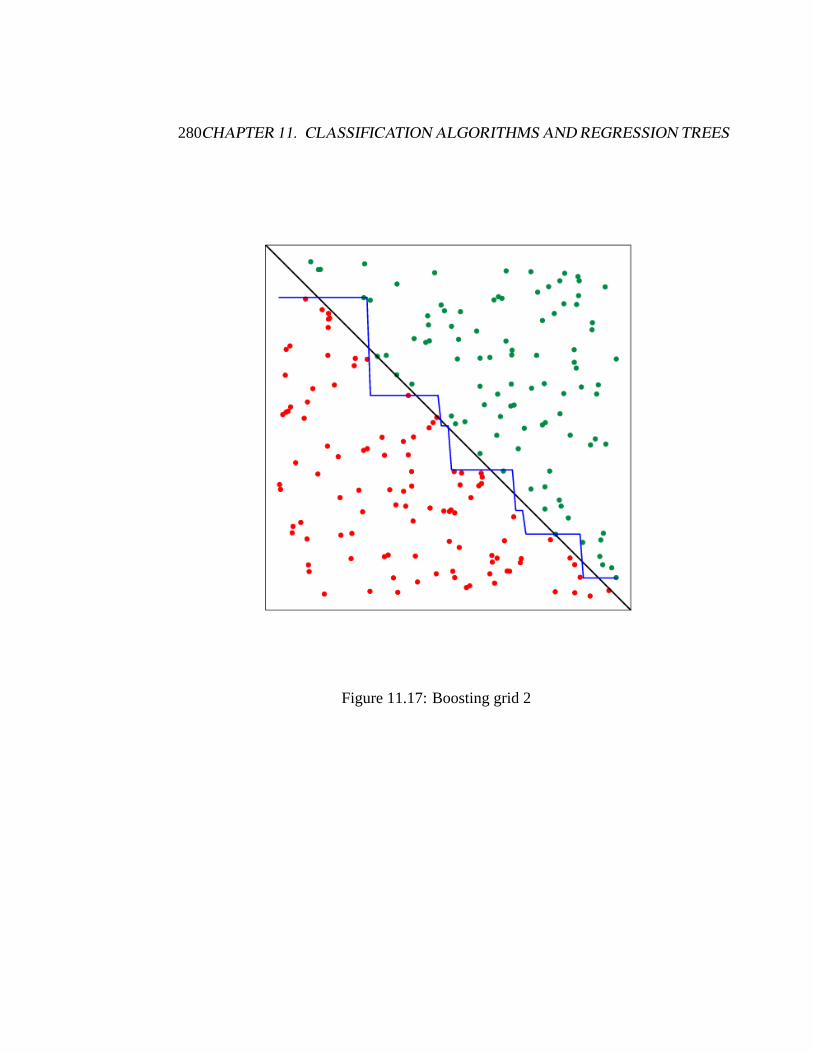
Figure 11.17: Boosting grid 2

chapter 11 classiﬁcation algorithms and regression trees · chapter 11 classiﬁcation algorithms...

Documents