chapter 10: metric path planning a. representations b. algorithms

10Chapter 10:

Metric Path Planning

a. Representationsb. Algorithms

Chapter 10: Metric Path Planning 2

10 Representing Area/Volume in Path Planning

• Quantitative or metric– Rep: Many different ways to represent an area

or volume of space• Looks like a “bird’s eye” view, position &

viewpoint independent– Algorithms

• Graph or network algorithms• Wavefront or graphics-derived algorithms


10 Metric Maps• Motivation for having a metric map is often path

planning (others include reasoning about space…)

• Determine a path from one point to goal– Generally interested in “best” or “optimal” What are measures

of best/optimal?

– Relevant: occupied or empty

• Path planning assumes an a priori map of relevant aspects– Only as good as last time map was updated


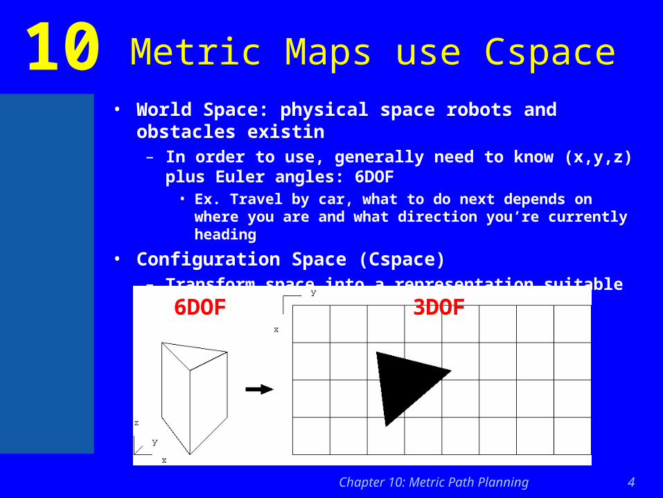
10 Metric Maps use Cspace• World Space: physical space robots and obstacles existin

– In order to use, generally need to know (x,y,z) plus Euler angles: 6DOF

• Ex. Travel by car, what to do next depends on where you are and what direction you’re currently heading

• Configuration Space (Cspace)– Transform space into a representation suitable for robots,

simplifying assumptions

6DOF 3DOF


10 Major Cspace Representations

• Idea: reduce physical space to a cspace representation which is more amenable for storage in computers and for rapid execution of algorithms

• Major types

– Meadow Maps

– Generalized Voronoi Graphs (GVG)

– Regular grids, quadtrees


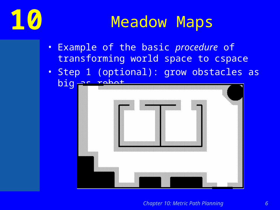
10 Meadow Maps

• Example of the basic procedure of transforming world space to cspace

• Step 1 (optional): grow obstacles as big as robot


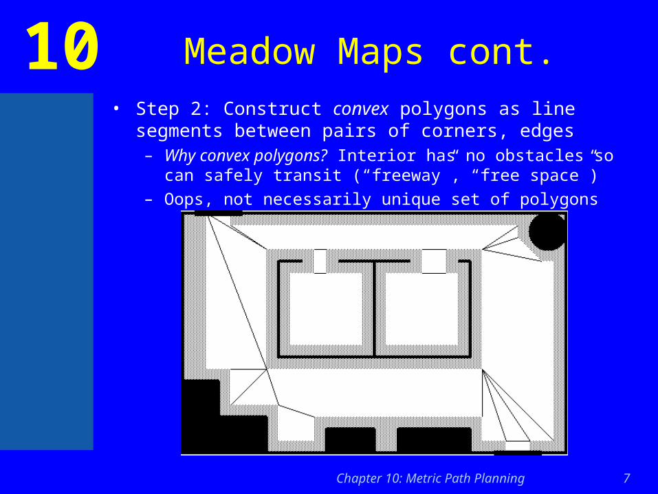
10 Meadow Maps cont.• Step 2: Construct convex polygons as line segments between pairs

of corners, edges– Why convex polygons? Interior has no obstacles so can safely transit

(“freeway”, “free space”)

– Oops, not necessarily unique set of polygons


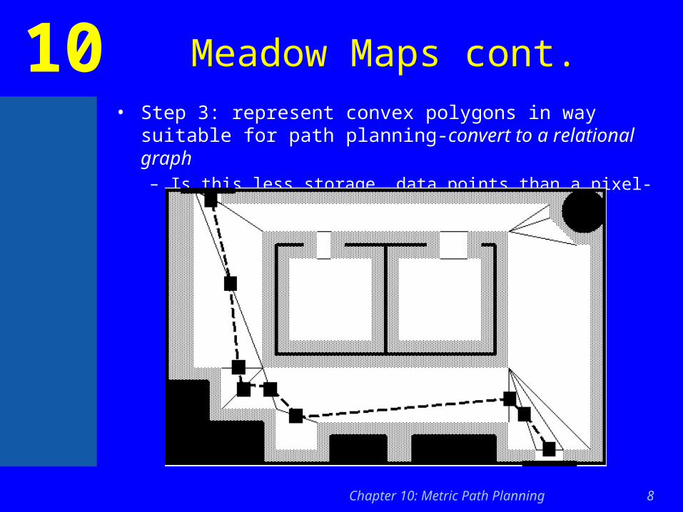
10 Meadow Maps cont.• Step 3: represent convex polygons in way suitable for path

planning-convert to a relational graph– Is this less storage, data points than a pixel-by-pixel representation?


10 Problems with Meadow Maps

• Not unique generation of polygons

• Could you actually create this type of map with sensor data?

• How does it tie into actually navigating the path?– How does robot recognize “right” corners, edges and go to

“middle”?

– What about sensor noise?


10 Path Relaxation

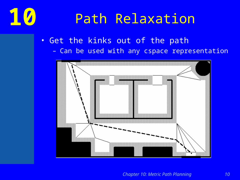
• Get the kinks out of the path– Can be used with any cspace representation


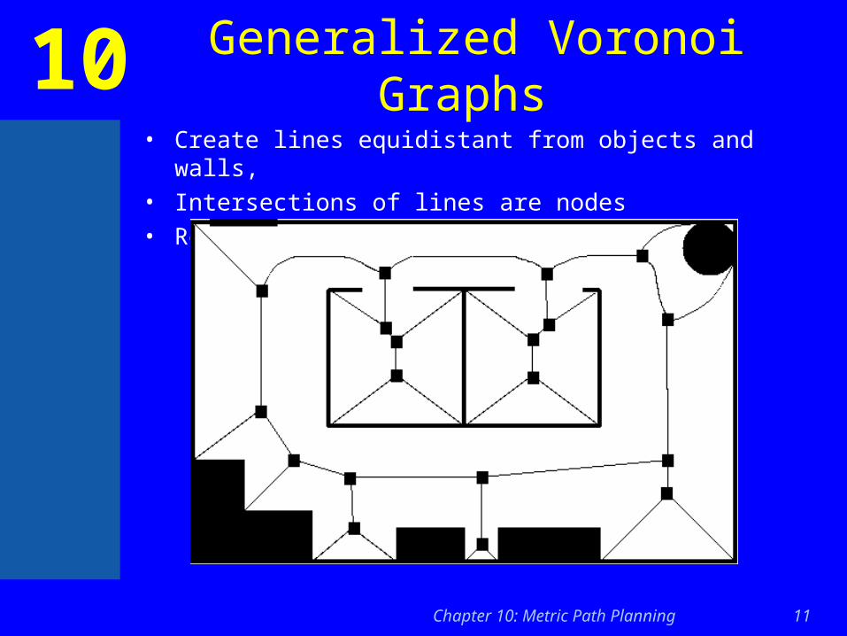
10 Generalized Voronoi Graphs • Create lines equidistant from objects and walls,

• Intersections of lines are nodes

• Result is a relational graph


10 Regular Grids

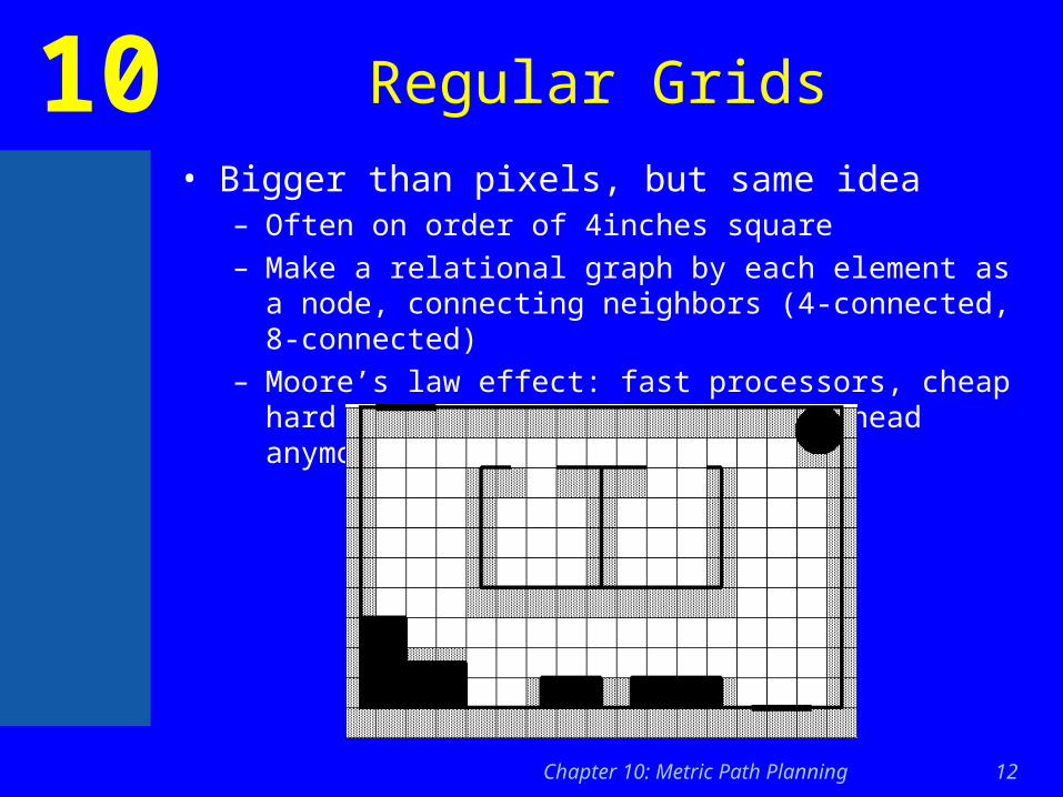
• Bigger than pixels, but same idea– Often on order of 4inches square

– Make a relational graph by each element as a node, connecting neighbors (4-connected, 8-connected)

– Moore’s law effect: fast processors, cheap hard drives, who cares about overhead anymore?


10 Problems with GVG and Regular Grids

• GVG– Sensitive to sensor noise

– Path execution requires robot to be able to sense boundaries

• Grids– World doesn’t always line up on grids

– Digitalization bias: left over space marked as occupied


10 Summary

• Metric path planning requires – Representation of world space, usually try to simplify to

cspace– Algorithms which can operate over representation to produce

best/optimal path

• Representation– Usually try to end up with relational graph– Regular grids are currently most popular in practice, GVGs

are interesting– Tricks of the trade

• Grow obstacles to size of robot to be able to treat holonomic robots as point

• Relaxation (string tightening)

• Metric methods often ignore issue of– how to execute a planned path– Impact of sensor noise or uncertainty, localization


10 Algorithms

• Path planning– A* for relational graphs

– Wavefront for operating directly on regular grids

• Interleaving Path Planning and Execution


10 Motivation for A*

• Single Source Shortest Path algorithms are exhaustive, visting all edges– Can’t we throw away paths when we see that they aren’t going

to the goal, rather than follow all branches?

• This means having a mechanism to “prune” branches as we go, rather than after full exploration

• Algorithms which prune earlier (but correctly) are preferred over algorithms which do it later.

• Issue: the mechanism for pruning


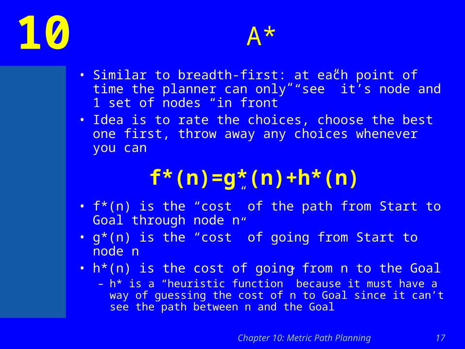
10 A*• Similar to breadth-first: at each point of time the

planner can only “see” it’s node and 1 set of nodes “in front”

• Idea is to rate the choices, choose the best one first, throw away any choices whenever you can

• f*(n) is the “cost” of the path from Start to Goal through node n

• g*(n) is the “cost” of going from Start to node n• h*(n) is the cost of going from n to the Goal

– h* is a “heuristic function” because it must have a way of guessing the cost of n to Goal since it can’t see the path between n and the Goal

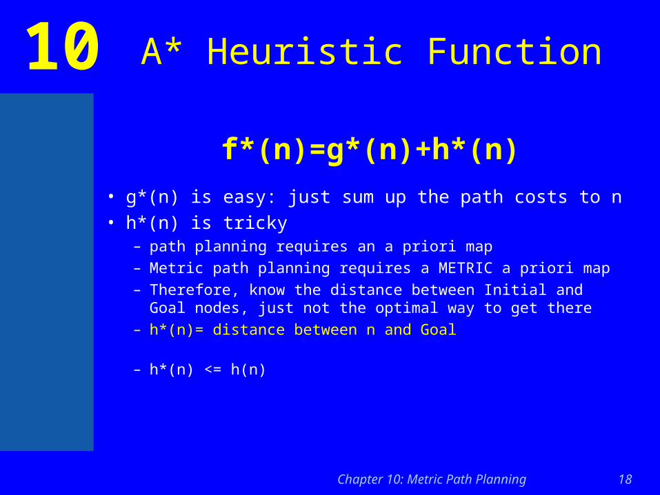
f*(n)=g*(n)+h*(n)


10 A* Heuristic Function

• g*(n) is easy: just sum up the path costs to n

• h*(n) is tricky– path planning requires an a priori map

– Metric path planning requires a METRIC a priori map

– Therefore, know the distance between Initial and Goal nodes, just not the optimal way to get there

– h*(n)= distance between n and Goal

– h*(n) <= h(n)

f*(n)=g*(n)+h*(n)


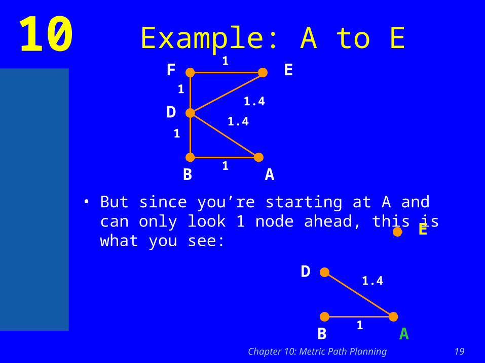
10 Example: A to E

• But since you’re starting at A and can only look 1 node ahead, this is what you see:

AB

D

F E

1

1

1

1

1.4

1.4

AB

D

E

1

1.4


10

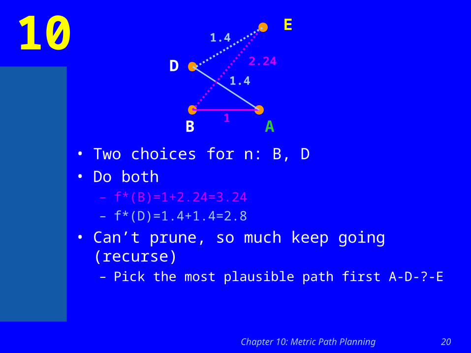
• Two choices for n: B, D

• Do both– f*(B)=1+2.24=3.24

– f*(D)=1.4+1.4=2.8

• Can’t prune, so much keep going (recurse)– Pick the most plausible path first A-D-?-E

AB

D

E

1

1.4

1.4

2.24


10

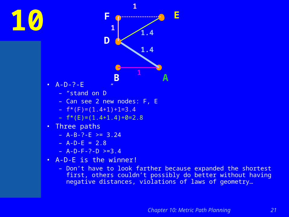
• A-D-?-E– “stand on D”– Can see 2 new nodes: F, E– f*(F)=(1.4+1)+1=3.4– f*(E)=(1.4+1.4)+0=2.8

• Three paths– A-B-?-E >= 3.24– A-D-E = 2.8– A-D-F-?-D >=3.4

• A-D-E is the winner! – Don’t have to look farther because expanded the shortest first, others couldn’t

possibly do better without having negative distances, violations of laws of geometry…

AB

D

E

1

1.4

1.4

F1

1


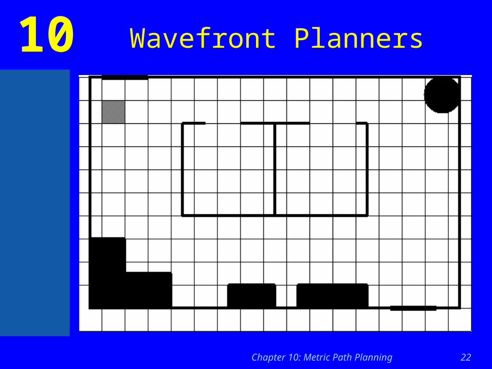
10 Wavefront Planners


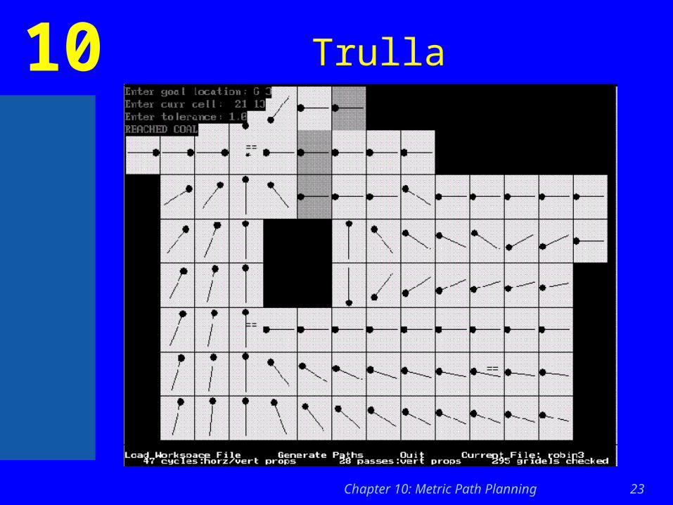
10 Trulla


10 Interleaving Path Planning and Reactive Execution

• Graph-based planners generate a path and subpaths or subsegments

• Recall NHC, AuRA– Pilot looks at current subpath, instantiates behaviors to get from

current location to subgoal

• When the robot tries to reach a subgoal, it may exhibit subgoal obsession due to an encoder error - it is necessary to allow a tolerance corresponding usually to +/- width of robot

• What happens if a goal is blocked? - need a Termination condition, e.g. deadline

• What happens if a robot avoiding an obstacle is now closer to the next subgoal? - it would be good to use an opportunistic replanning


10 Two Example Approaches

• If computing all possible paths in advance, there not a problem– Shortest path between pairs will be part of

shortest path to more distant pairs

• D* – Run A* over all possible pairs of nodes

– continuously update the map

– disadvantages: 1. too computationally expensive to be practical for a robot 2. continuous replanning is highly dependent on sensing quality,


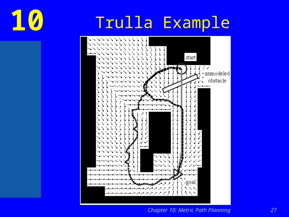
10 Two Example Approaches– Event driven scheme - event noticeable by

a reactive system would trigger replanning

– the Trulla planner uses for this dot product of the intended path vector and the actual path vector

– By-product of wave propagation style is path to everywhere

– for opportunistic replanning in case of favorable change D* is better, because it will automatically notice the change, while Trulla will not notice it


10 Trulla Example


10 Summary

• Metric path planners– graph-based (A* is best known)

– Wavefront

• Graph-based generate paths and subgoals.– Good for NHC styles of control

– In practice leads to:• Subgoal obsession

• Termination conditions

• Planning all possible paths helps with subgoal obsession– What happens when the map is wrong, things change, missed

opportunities? How can you tell when the map is wrong or that’s it worth the computation?


10 You should be able to:

• Define Cspace, path relaxation, digitization bias, subgoal obsession, termination condition

• Explain the difference between graph and wavefront planners

• Represent an indoor environment with a GVG, a regular grid, or a quadtree, and create a graph suitable for path planning

• Apply A* search

• Apply wavefront propagation

• Explain the differences between continuous and event-driven replanning

chapter 10: metric path planning a. representations b. algorithms

Documents