chapter 10 aggregate demand i - meltem daysal · 2009-08-30 · learning objectives ... is-lm model...
TRANSCRIPT
1
CHAPTER 10 0
Chapter 10
Aggregate Demand I
2
CHAPTER 10 1
3
CHAPTER 10 2
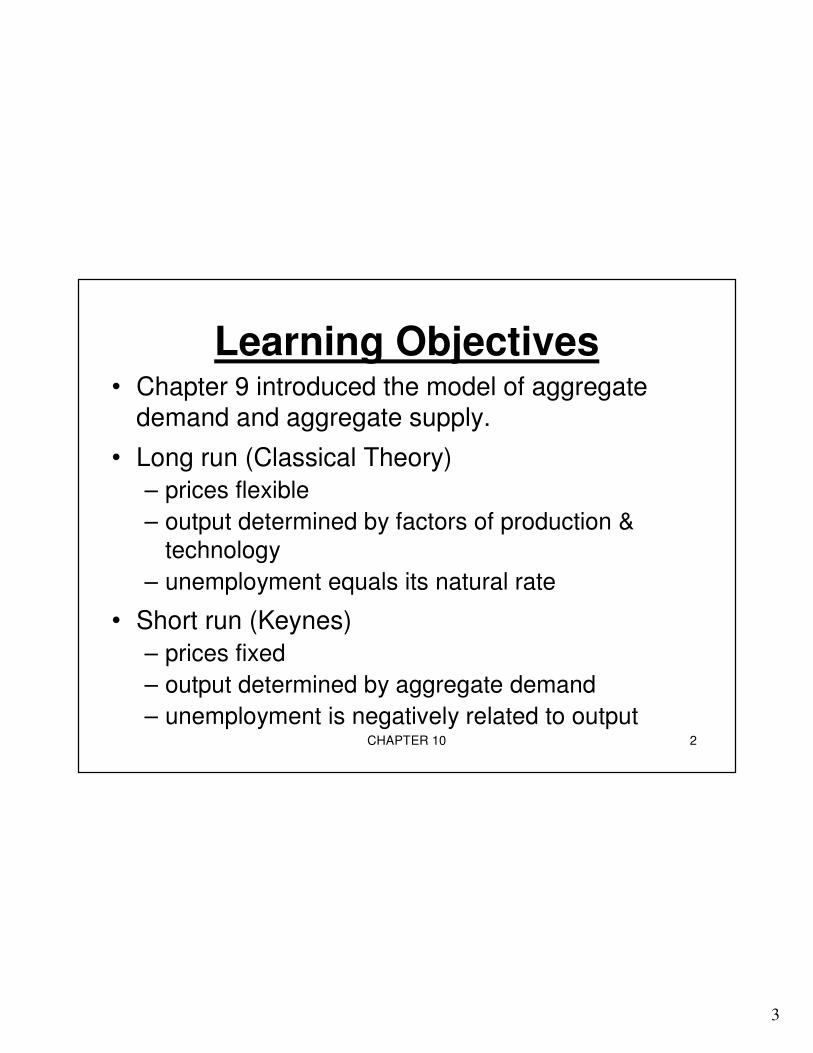
Learning Objectives• Chapter 9 introduced the model of aggregate
demand and aggregate supply.
• Long run (Classical Theory)
– prices flexible
– output determined by factors of production &
technology
– unemployment equals its natural rate
• Short run (Keynes)
– prices fixed
– output determined by aggregate demand
– unemployment is negatively related to output

4
CHAPTER 10 3
Learning Objectives• This chapter develops the IS-LM model
(Hicks), the theory that yields the aggregate demand curve.
• We focus on the short run and assume the price level is fixed.
5
CHAPTER 10 4
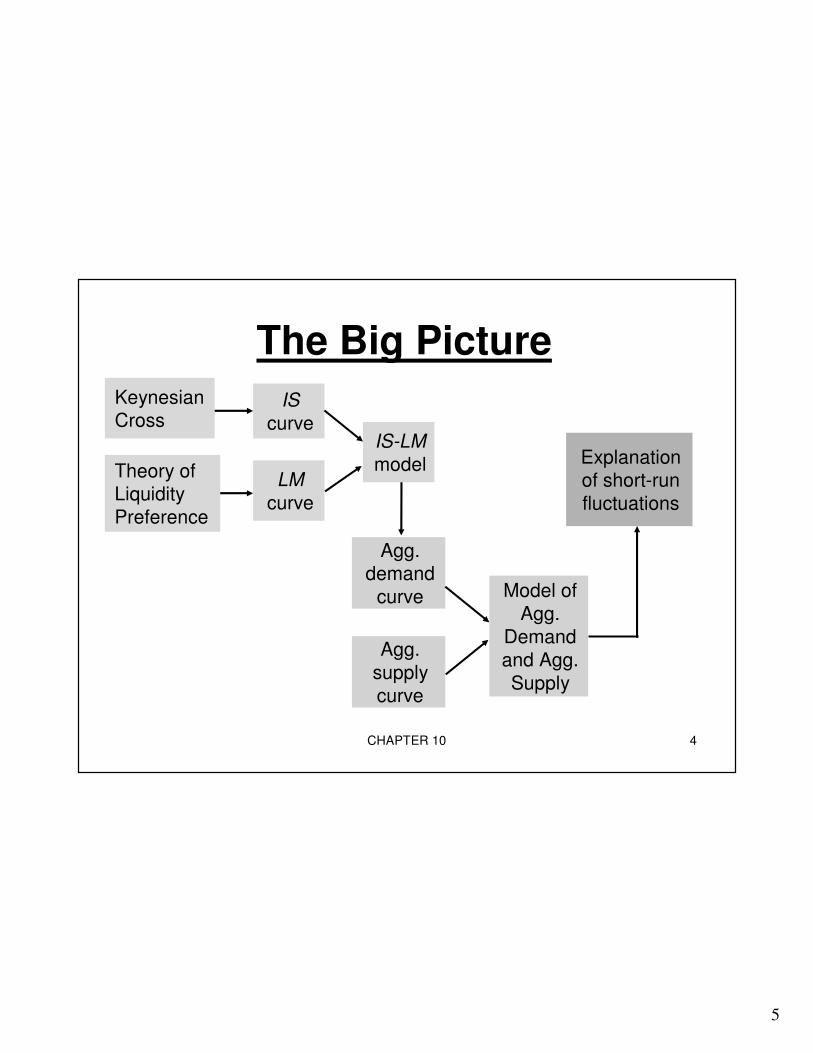
The Big Picture
KeynesianCross
Theory of Liquidity
Preference
IS
curve
LM
curve
IS-LM
model
Agg. demand
curve
Agg.
supply
curve
Model of
Agg.
Demand
and Agg.
Supply
Explanation of short-run
fluctuations
6
CHAPTER 10 5
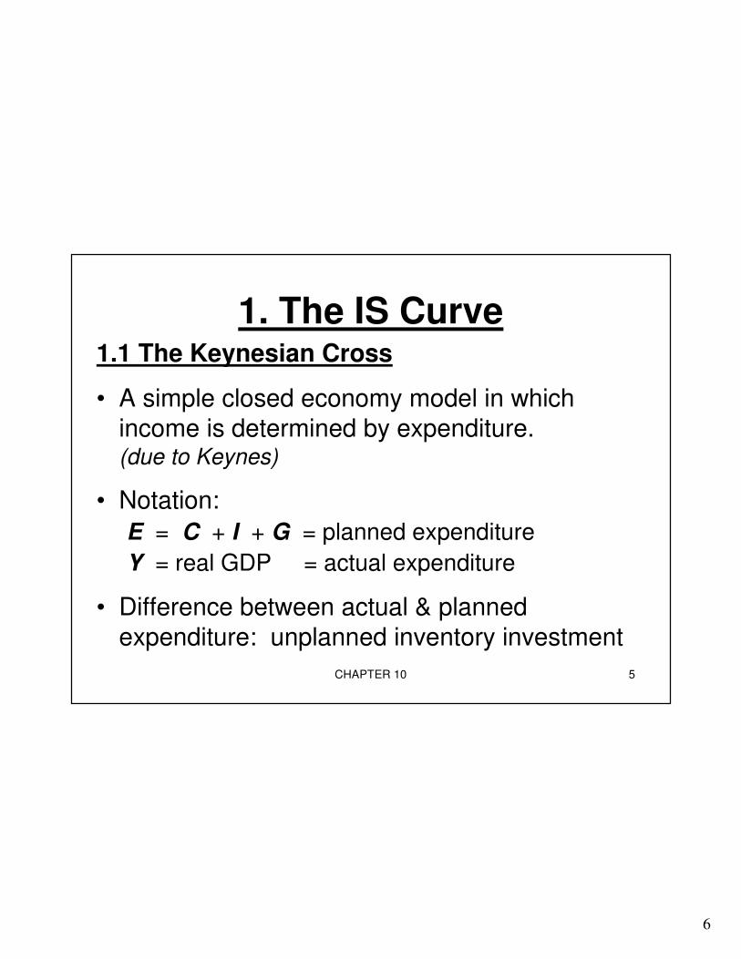
1. The IS Curve1.1 The Keynesian Cross
• A simple closed economy model in which
income is determined by expenditure. (due to Keynes)
• Notation:
E = C + I + G = planned expenditure
Y = real GDP = actual expenditure
• Difference between actual & planned
expenditure: unplanned inventory investment
7
CHAPTER 10 6
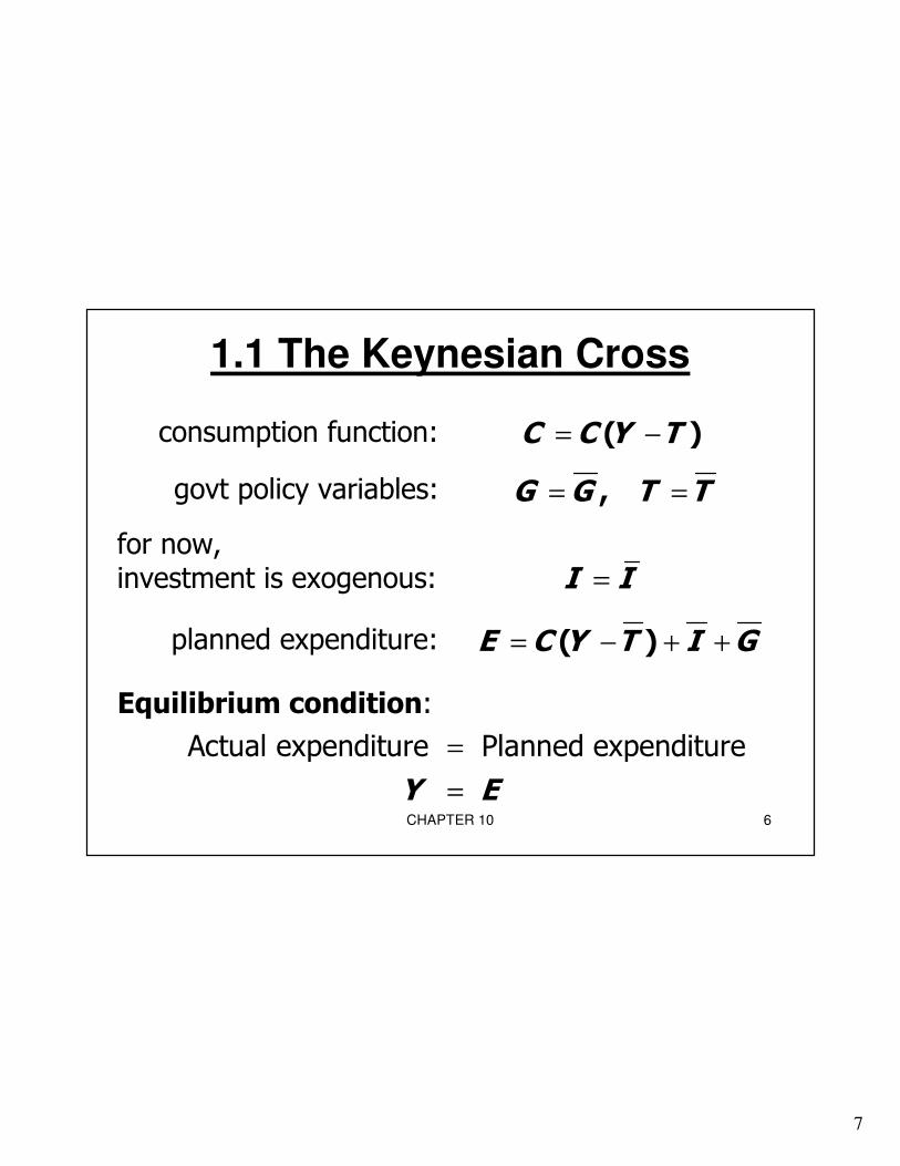
1.1 The Keynesian Cross
( )C C Y T= −
I I=
,G G T T= =
( )E C Y T I G= − + +
Actual expenditure Planned expenditure
Y E
=
=
consumption function:
for now, investment is exogenous:
planned expenditure:
Equilibrium condition:
govt policy variables:
8
CHAPTER 10 7
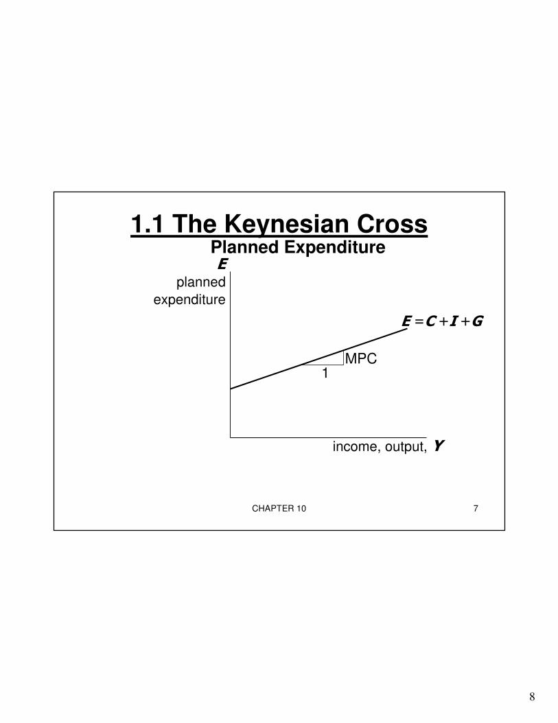
1.1 The Keynesian CrossPlanned Expenditure
income, output, Y
Eplanned
expenditure
E =C +I +G
MPC1
9
CHAPTER 10 8
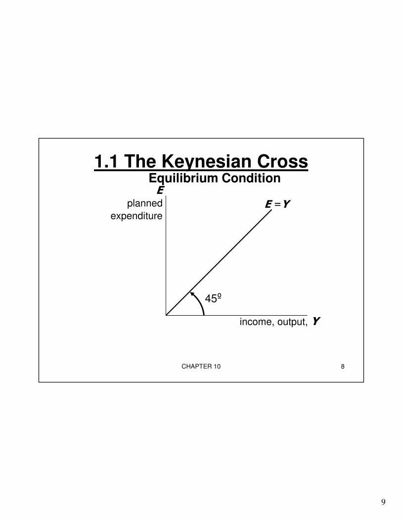
1.1 The Keynesian Cross Equilibrium Condition
income, output, Y
Eplanned
expenditureE =Y
45º
10
CHAPTER 10 9
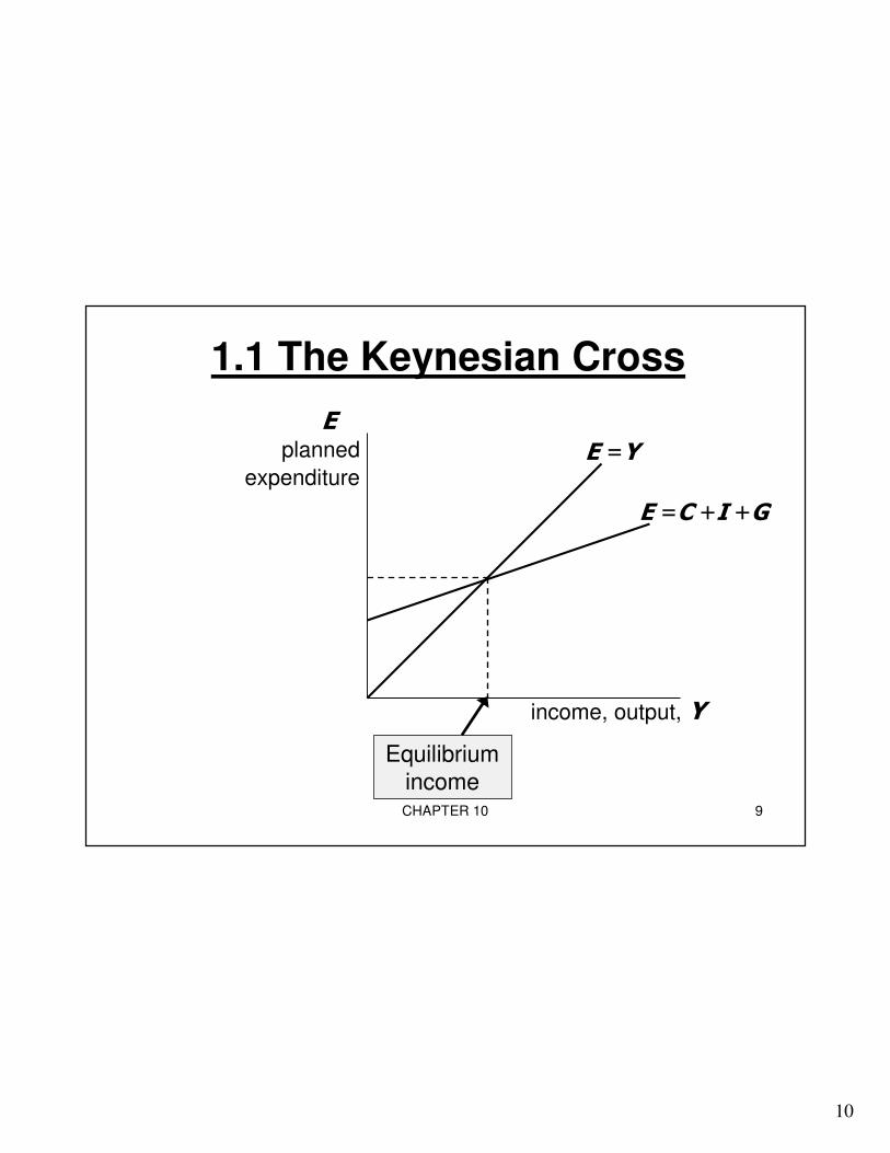
1.1 The Keynesian Cross
income, output, Y
Eplanned
expenditureE =Y
E =C +I +G
Equilibrium
income
11
CHAPTER 10 10
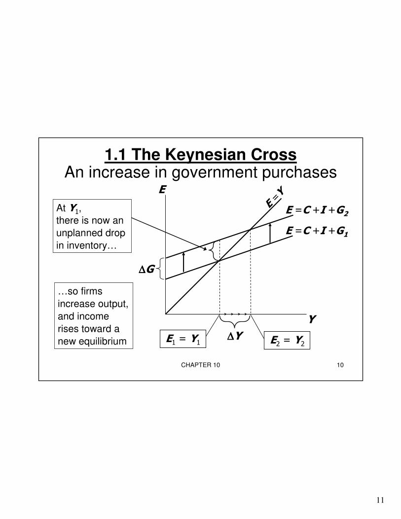
1.1 The Keynesian CrossAn increase in government purchases
Y
E
E
=
Y
E =C +I +G1
E1 = Y1
E =C +I +G2
E2 = Y2∆∆∆∆Y
At Y1,
there is now an
unplanned drop
in inventory…
…so firms
increase output,
and income
rises toward a
new equilibrium
∆∆∆∆G
12
CHAPTER 10 11
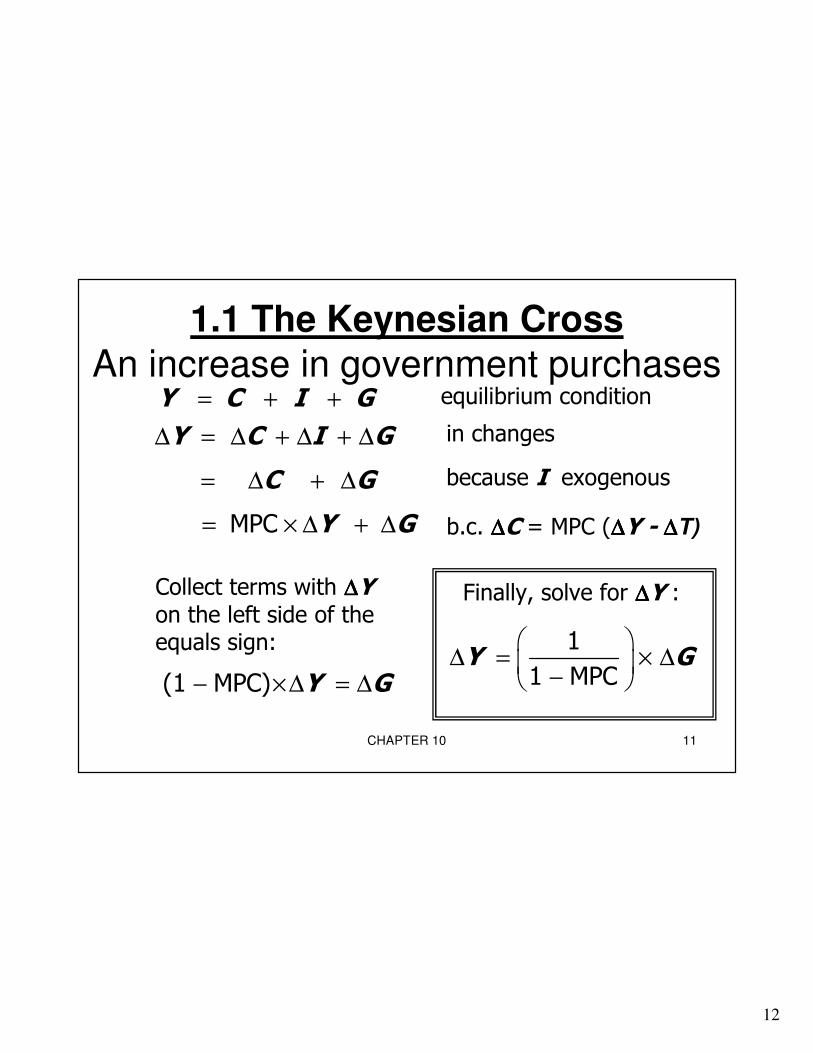
1.1 The Keynesian Cross
An increase in government purchasesY C I G= + +
Y C I G∆ = ∆ + ∆ + ∆
MPC Y G= × ∆ + ∆
C G= ∆ + ∆
(1 MPC) Y G− ×∆ = ∆
1
1 MPCY G
∆ = × ∆ −
equilibrium condition
in changes
because I exogenous
b.c. ∆∆∆∆C = MPC (∆∆∆∆Y - ∆∆∆∆T)
Collect terms with ∆∆∆∆Yon the left side of the equals sign:
Finally, solve for ∆∆∆∆Y :
13
CHAPTER 10 12
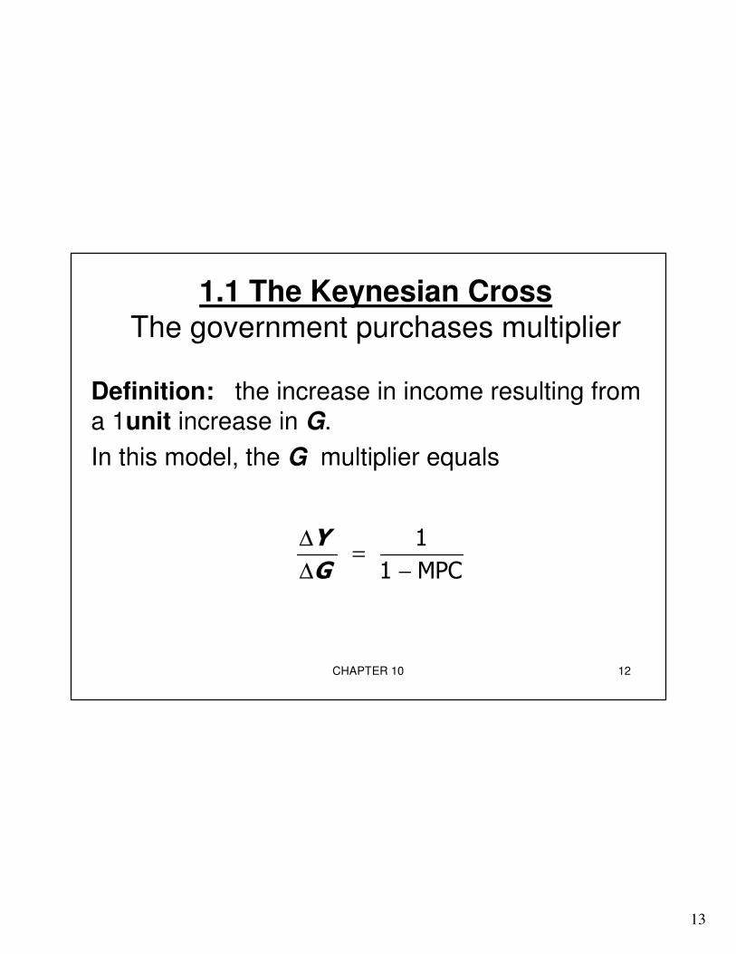
1.1 The Keynesian Cross
The government purchases multiplier
Definition: the increase in income resulting from
a 1unit increase in G.
In this model, the G multiplier equals
1
1 MPC
Y
G
∆=
∆ −
14
CHAPTER 10 13
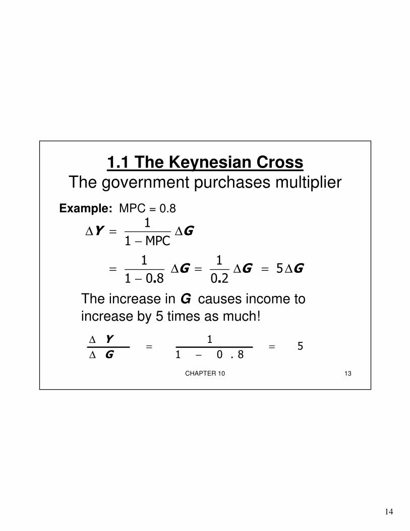
1.1 The Keynesian Cross
The government purchases multiplier
Example: MPC = 0.8
1
1 MPC
1 15
1 0 8 0 2. .
Y G
G G G
∆ = ∆−
= ∆ = ∆ = ∆−
The increase in G causes income to
increase by 5 times as much!
15
1 0 . 8
Y
G
∆= =
∆ −
15
CHAPTER 10 14
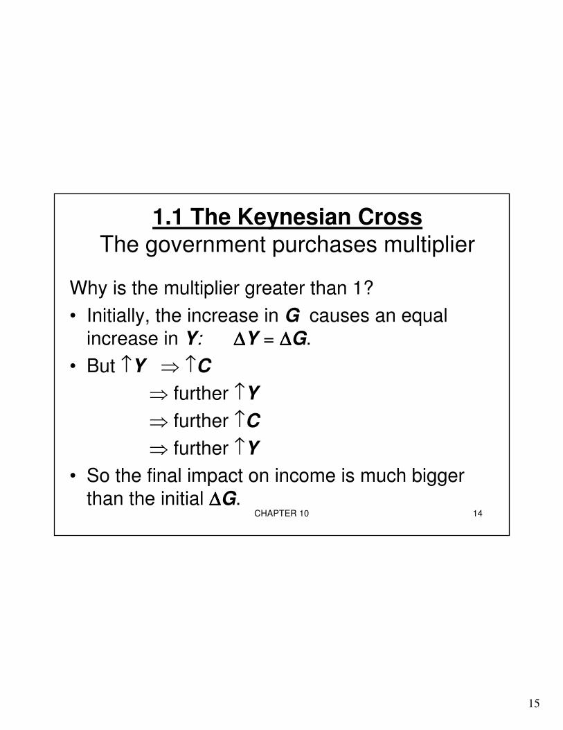
1.1 The Keynesian Cross
The government purchases multiplier
Why is the multiplier greater than 1?
• Initially, the increase in G causes an equal
increase in Y: ∆∆∆∆Y = ∆∆∆∆G.
• But ↑Y ⇒ ↑C
⇒ further ↑Y
⇒ further ↑C
⇒ further ↑Y
• So the final impact on income is much bigger
than the initial ∆∆∆∆G.
16
CHAPTER 10 15
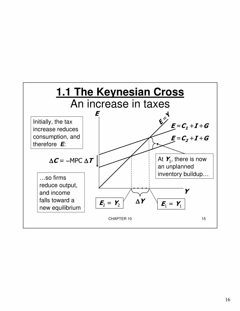
1.1 The Keynesian CrossAn increase in taxes
Y
E
E
=
Y
E =C2 +I +G
E2 = Y2
E =C1 +I +G
E1 = Y1∆∆∆∆Y
At Y1, there is now
an unplanned
inventory buildup……so firms
reduce output,
and income
falls toward a
new equilibrium
∆∆∆∆C = −−−−MPC ∆∆∆∆T
Initially, the tax
increase reduces
consumption, and
therefore E:
17
CHAPTER 10 16
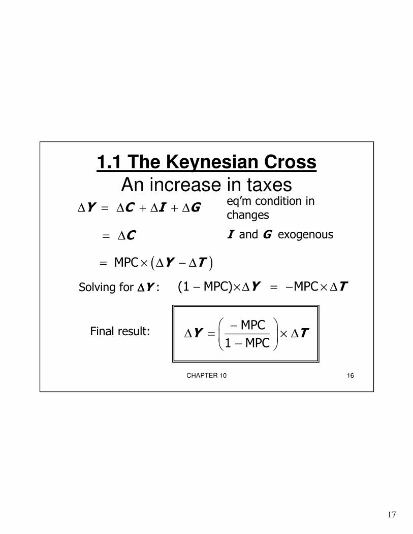
1.1 The Keynesian Cross
An increase in taxesY C I G∆ = ∆ + ∆ + ∆
( )MPC Y T= × ∆ − ∆
C= ∆
(1 MPC) MPCY T− ×∆ = − × ∆
eq’m condition in changes
I and G exogenous
Solving for ∆∆∆∆Y :
MPC
1 MPCY T
−∆ = × ∆ −
Final result:
18
CHAPTER 10 17
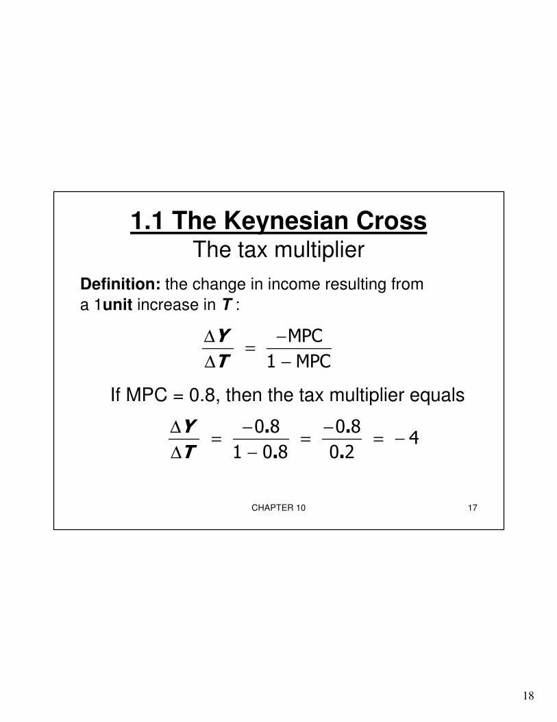
1.1 The Keynesian CrossThe tax multiplier
Definition: the change in income resulting from
a 1unit increase in T :
MPC
1 MPC
Y
T
∆ −=
∆ −
0 8 0 84
1 0 8 0 2
. .
. .
Y
T
∆ − −= = = −
∆ −
If MPC = 0.8, then the tax multiplier equals

19
CHAPTER 10 18
1.1 The Keynesian CrossThe tax multiplier
…is negative:
An increase in taxes reduces consumer
spending, which reduces equilibrium income.
…is greater than one (in absolute value):
A change in taxes has a multiplier effect on
income.
…is smaller than the govt spending multiplier:
Consumers save the fraction (1-MPC) of a tax
cut, so the initial boost in spending from a tax cut
is smaller than from an equal increase in G.
20
CHAPTER 10 19
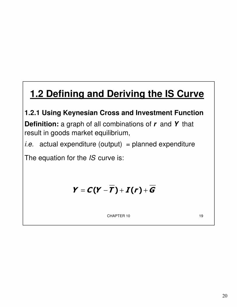
1.2 Defining and Deriving the IS Curve
1.2.1 Using Keynesian Cross and Investment Function
Definition: a graph of all combinations of r and Y that
result in goods market equilibrium,
i.e. actual expenditure (output) = planned expenditure
The equation for the IS curve is:
( ) ( )Y C Y T I r G= − + +
21
CHAPTER 10 20
Y2Y1
Y2Y1
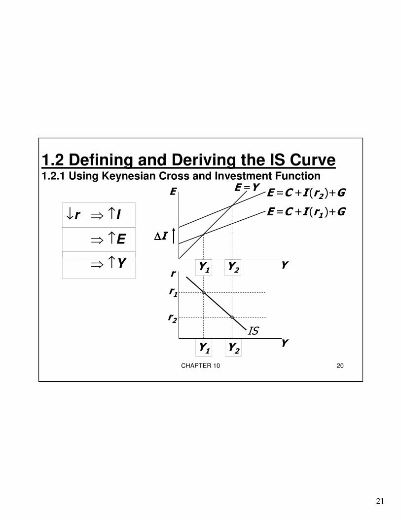
1.2 Defining and Deriving the IS Curve1.2.1 Using Keynesian Cross and Investment Function
↓r ⇒ ↑I
Y
E
r
Y
E =C +I (r1 )+G
E =C +I (r2 )+G
r1
r2
E =Y
IS
∆∆∆∆I⇒ ↑E
⇒ ↑Y
22
CHAPTER 10 21
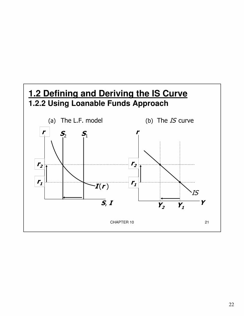
1.2 Defining and Deriving the IS Curve1.2.2 Using Loanable Funds Approach
S, I
r
I (r )r1
r2
r
YY1
r1
r2
(a) The L.F. model (b) The IS curve
Y2
S1S2
IS
23
CHAPTER 10 22
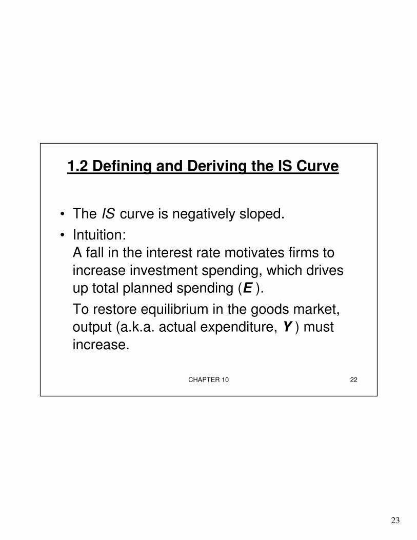
1.2 Defining and Deriving the IS Curve
• The IS curve is negatively sloped.
• Intuition:
A fall in the interest rate motivates firms to
increase investment spending, which drives
up total planned spending (E ).
To restore equilibrium in the goods market,
output (a.k.a. actual expenditure, Y ) must
increase.
24
CHAPTER 10 23
1.3 Fiscal Policy and the IS Curve
• We can use the IS-LM model to see
how fiscal policy (G and T ) can affect aggregate demand and output.
• Let’s start by using the Keynesian Cross
to see how fiscal policy shifts the IScurve…
25
CHAPTER 10 24
Y2Y1
Y2Y1
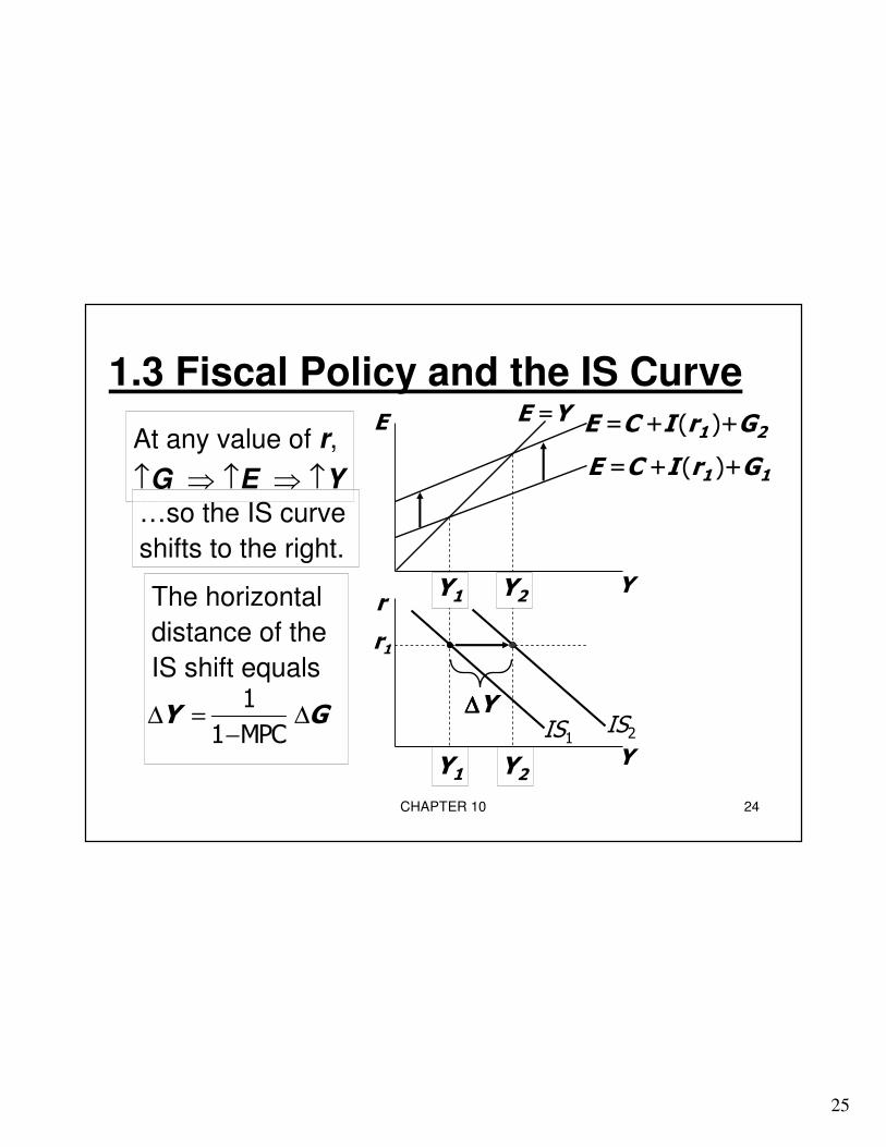
1.3 Fiscal Policy and the IS Curve
At any value of r,
↑G ⇒ ↑E ⇒ ↑Y
Y
E
r
Y
E =C +I (r1 )+G1
E =C +I (r1 )+G2
r1
E =Y
IS1
The horizontal
distance of the
IS shift equals
IS2
…so the IS curve
shifts to the right.
1
1 MPCY G∆ = ∆
−∆∆∆∆Y
26
CHAPTER 10 25
2. The LM Curve
2.1 The Theory of Liquidity Preference
• A simple theory in which the interest rate
is determined by money supply and money demand. (due to Keynes again)
27
CHAPTER 10 26
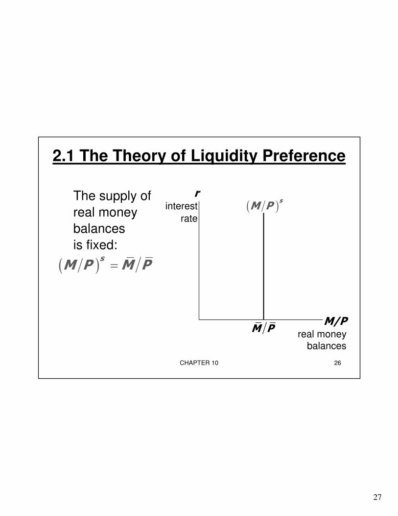
2.1 The Theory of Liquidity Preference
The supply of
real money
balances
is fixed:
( )sM P M P=
M/Preal money
balances
rinterest
rate( )sM P
M P
28
CHAPTER 10 27
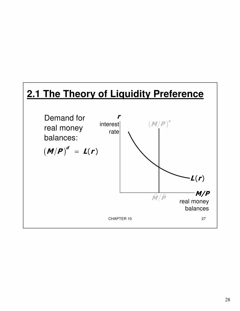
2.1 The Theory of Liquidity Preference
Demand for
real money
balances:
M/Preal money
balances
rinterest
rate( )sM P
M P
( ) ( )d
M P L r=
L (r )
29
CHAPTER 10 28
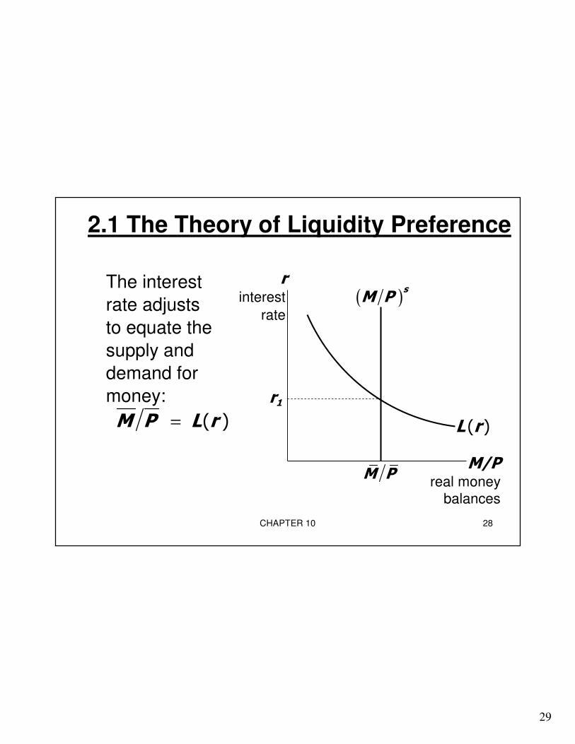
2.1 The Theory of Liquidity Preference
The interest
rate adjusts
to equate the
supply and
demand for
money:
M/Preal money
balances
rinterest
rate( )sM P
M P
( )M P L r= L (r )
r1
30
CHAPTER 10 29
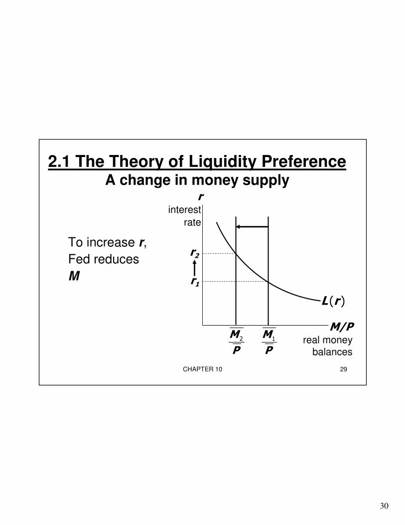
2.1 The Theory of Liquidity PreferenceA change in money supply
To increase r,
Fed reduces
M
M/Preal money
balances
rinterest
rate
1M
P
L (r )
r1
r2
2M
P
31
CHAPTER 10 30
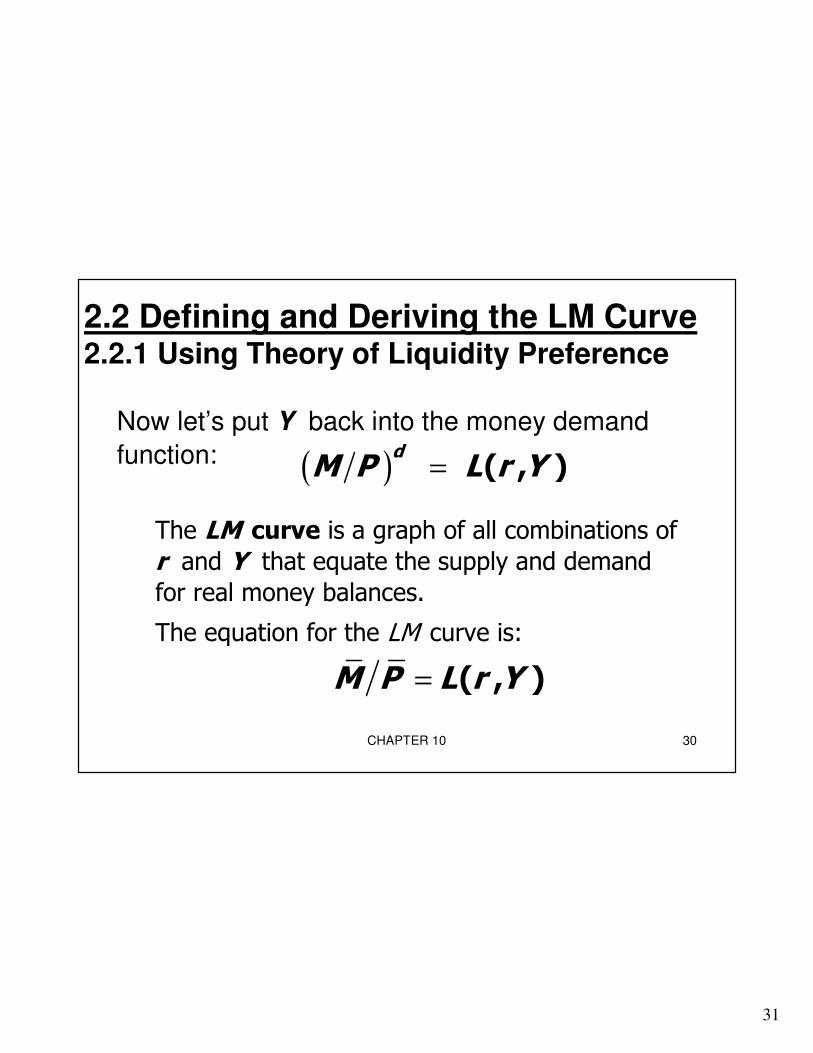
2.2 Defining and Deriving the LM Curve2.2.1 Using Theory of Liquidity Preference
Now let’s put Y back into the money demand
function:
( , )M P L r Y=
The LM curve is a graph of all combinations of
r and Y that equate the supply and demand
for real money balances.
The equation for the LM curve is:
( )dM P L r Y= ( , )
32
CHAPTER 10 31
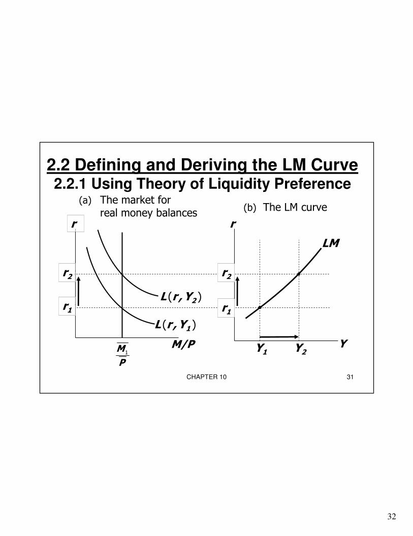
2.2 Defining and Deriving the LM Curve2.2.1 Using Theory of Liquidity Preference
M/P
r
1M
P
L (r ,Y1 )
r1
r2
r
YY1
r1L (r ,Y2 )
r2
Y2
LM
(a) The market for real money balances
(b) The LM curve
33
CHAPTER 10 32
2.2 Defining and Deriving the LM Curve2.2.2 Using Quantity Equation
• Quantity Equation
MV=PY
• Quantity Theory of money assumes constant velocity � vertical LM curve
• If we adjust it so that V=V(r) then we get the upward sloping LM curve again.
34
CHAPTER 10 33
2.2 Defining and Deriving the LM
Curve• The LM curve is positively sloped.
• Intuition:
An increase in income raises money
demand.
Since the supply of real balances is fixed,
there is now excess demand in the
money market at the initial interest rate.
The interest rate must rise to restore
equilibrium in the money market.
35
CHAPTER 10 34
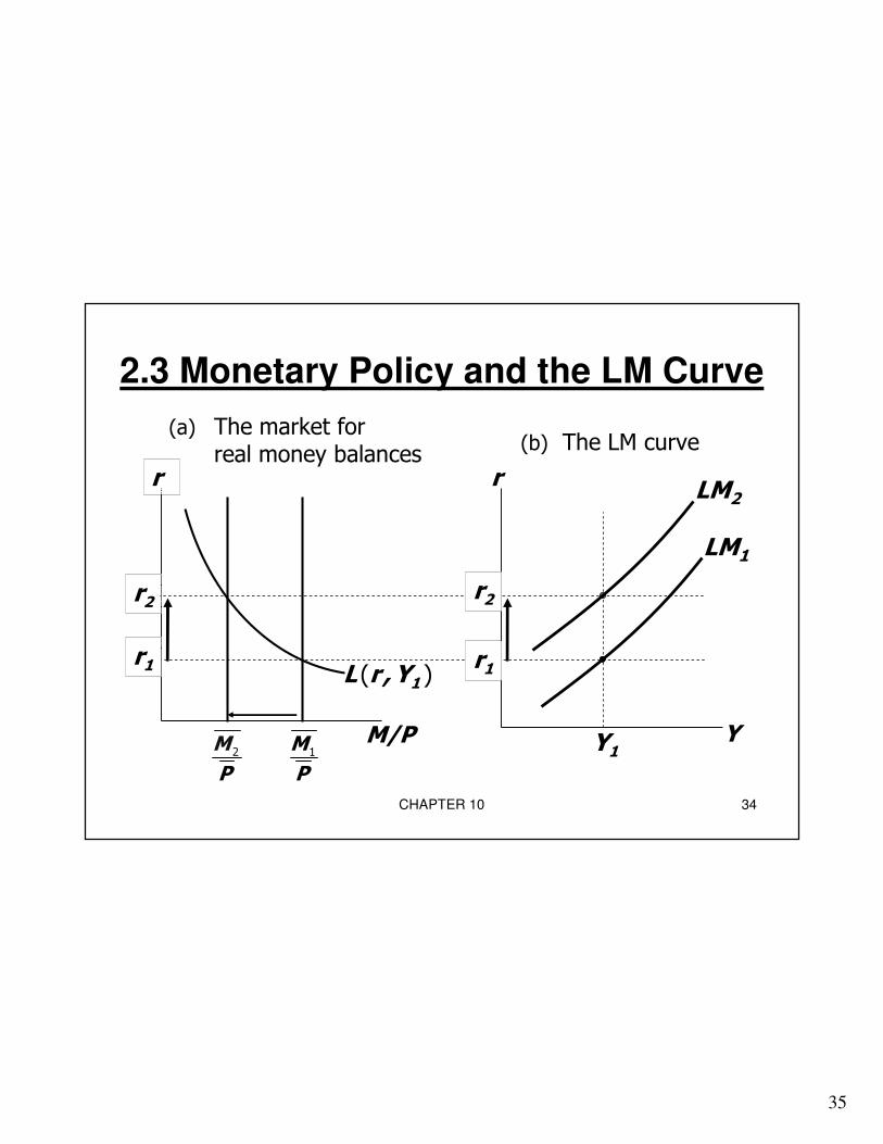
2.3 Monetary Policy and the LM Curve
M/P
r
1M
P
L (r ,Y1 )r1
r2
r
YY1
r1
r2
LM1
(a) The market for real money balances
(b) The LM curve
2M
P
LM2
36
CHAPTER 10 35
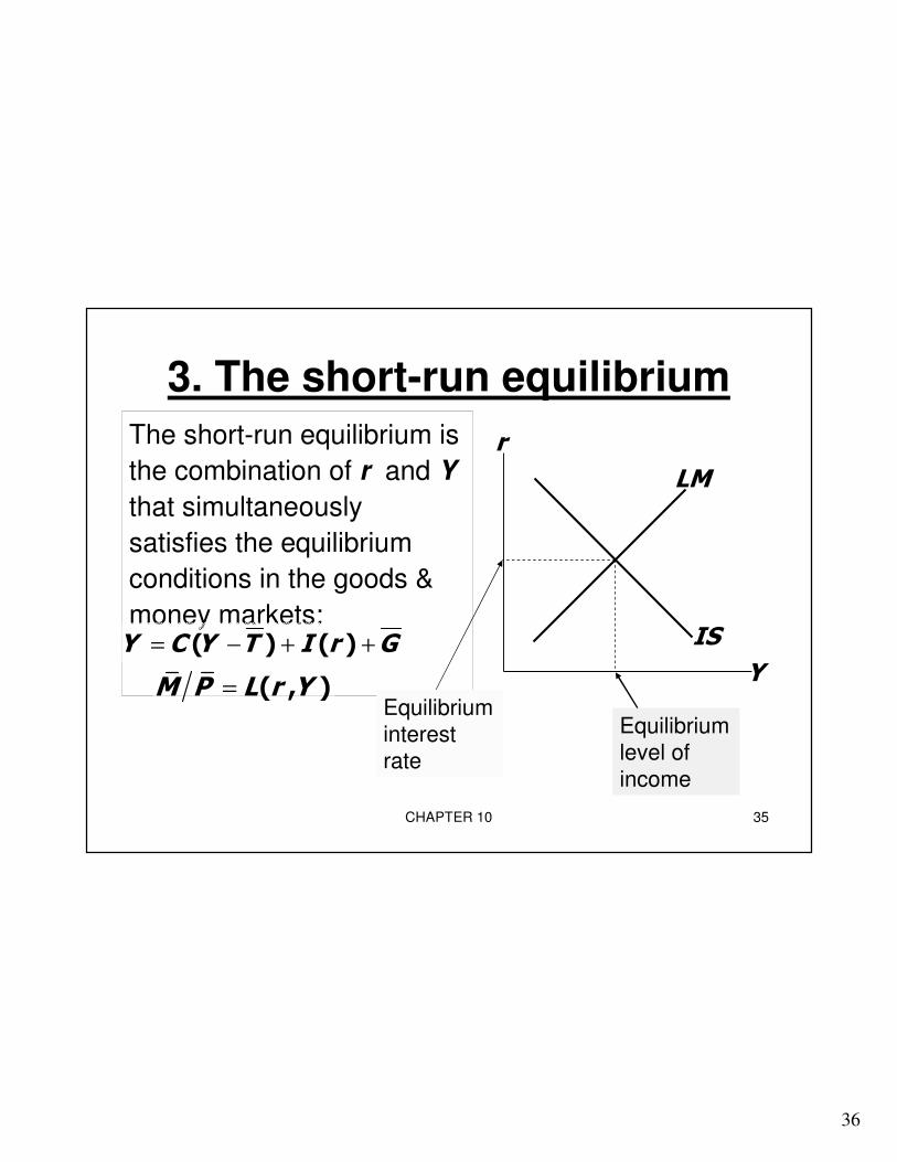
3. The short-run equilibrium
The short-run equilibrium is
the combination of r and Y
that simultaneously
satisfies the equilibrium
conditions in the goods &
money markets: ( ) ( )Y C Y T I r G= − + +
Y
r
( , )M P L r Y=
IS
LM
Equilibriuminterestrate
Equilibriumlevel of
income
37
CHAPTER 10 36
Chapter summary1. Keynesian Cross
� basic model of income determination
� takes fiscal policy & investment as exogenous
� fiscal policy has a multiplied impact on
income.
2. IS curve
� comes from Keynesian Cross when planned
investment depends negatively on interest rate
� shows all combinations of r and Y that
equate planned expenditure with actual
expenditure on goods & services
38
CHAPTER 10 37
Chapter summary3. Theory of Liquidity Preference
� basic model of interest rate determination
� takes money supply & price level as
exogenous
� an increase in the money supply lowers the
interest rate
4. LM curve
� comes from Liquidity Preference Theory when
money demand depends positively on income
� shows all combinations of r andY that equate
demand for real money balances with supply
39
CHAPTER 10 38
Chapter summary5. IS-LM model
� Intersection of IS and LM curves shows the
unique point (Y, r ) that satisfies equilibrium in
both the goods and money markets.

40
CHAPTER 10 39
Preview of Chapter 11In Chapter 11, we will
� use the IS-LM model to analyze the impact of policies and shocks
� learn how the aggregate demand curve comes from IS-LM
� use the IS-LM and AD-AS models together to analyze the short-run and long-run effects of shocks
� learn about the Great Depression using our models