Chapter 10: A Hilbert Space Approach To

Variance Reduction

Roberto Szechtman

Department of Operations Research, Naval Postgraduate School

Abstract

In this chapter we explain variance reduction techniques from the Hilbert spacestandpoint, in the terminating simulation context. We use projection ideas to ex-plain how variance is reduced, and to link different variance reduction techniques.Our focus is on the methods of control variates, conditional Monte Carlo, weightedMonte Carlo, stratification, and Latin hypercube sampling.

1 Introduction

The goal of this chapter is to describe variance reduction techniques from aHilbert space perspective in the terminating simulation setting, with the fo-cal point lying on the method of control variates. Several variance reductiontechniques have an intuitive geometric interpretation in the Hilbert space set-ting, and it is often possible to obtain rather deep probabilistic results withrelatively little effort by framing the relevant mathematical objects in an ap-propriate Hilbert space. The procedure employed to reach most results in thiscontext consists of three stages:

(1) Find a pertinent space endowed with an inner product.(2) Apply Hilbert space results towards a desired conclusion.(3) Translate the conclusions back into probabilistic language.

The key geometric idea used in Stage 2 is that of “projection”: Given anelement y in a Hilbert space H and a subset M of the Hilbert space, it holdsunder mild conditions that there exists a unique element in M that is closestto y. The characterization of this element depends on the space H determined

Email address: rszechtm@nps.edu (Roberto Szechtman).

Preprint submitted to Elsevier Science 16 November 2005

Report Documentation Page Form ApprovedOMB No. 0704-0188

Public reporting burden for the collection of information is estimated to average 1 hour per response, including the time for reviewing instructions, searching existing data sources, gathering andmaintaining the data needed, and completing and reviewing the collection of information. Send comments regarding this burden estimate or any other aspect of this collection of information,including suggestions for reducing this burden, to Washington Headquarters Services, Directorate for Information Operations and Reports, 1215 Jefferson Davis Highway, Suite 1204, ArlingtonVA 22202-4302. Respondents should be aware that notwithstanding any other provision of law, no person shall be subject to a penalty for failing to comply with a collection of information if itdoes not display a currently valid OMB control number.

1. REPORT DATE 16 NOV 2005

2. REPORT TYPE N/A

3. DATES COVERED -

4. TITLE AND SUBTITLE Chapter 10: A Hilbert Space Approach To Variance Reduction

5a. CONTRACT NUMBER

5b. GRANT NUMBER

5c. PROGRAM ELEMENT NUMBER

6. AUTHOR(S) 5d. PROJECT NUMBER

5e. TASK NUMBER

5f. WORK UNIT NUMBER

7. PERFORMING ORGANIZATION NAME(S) AND ADDRESS(ES) Naval Postgraduate School Department of Operations ResearchMonterey, CA 93943

8. PERFORMING ORGANIZATIONREPORT NUMBER

9. SPONSORING/MONITORING AGENCY NAME(S) AND ADDRESS(ES) 10. SPONSOR/MONITOR’S ACRONYM(S)

11. SPONSOR/MONITOR’S REPORT NUMBER(S)

12. DISTRIBUTION/AVAILABILITY STATEMENT Approved for public release, distribution unlimited

13. SUPPLEMENTARY NOTES Elsevier Handbooks in Operations Research and Management Science: Simulation (edited by S.G.Henderson and B.L. Nelson), Elsevier, Amsterdam, 259-289

14. ABSTRACT In this chapter we explain variance reduction techniques from the Hilbert space standpoint, in theterminating simulation context. We use projection ideas to explain how variance is reduced, and to linkdifferent variance reduction techniques. Our focus is on the methods of control variates, conditional MonteCarlo, weighted Monte Carlo, stratification, and Latin hypercube sampling.

15. SUBJECT TERMS

16. SECURITY CLASSIFICATION OF: 17. LIMITATION OF ABSTRACT

SAR

18. NUMBEROF PAGES

32

19a. NAME OFRESPONSIBLE PERSON

a. REPORT unclassified

b. ABSTRACT unclassified

c. THIS PAGE unclassified

Standard Form 298 (Rev. 8-98) Prescribed by ANSI Std Z39-18

by Stage 1, on y, and on M ; in essence it is found by dropping a perpendicularfrom y to M .

The Hilbert space explanation of control variates, and to a somewhat lesserextent that of conditional Monte Carlo, is closely related to that of othervariance reduction techniques; in this chapter we bridge these connectionswhenever they arise. From the projection perspective, it is often possible tolink variance reduction techniques for which the relevant Hilbert space H andelement y ∈ H are the same. The articulation is done by judiciously choosingthe subset M for each particular technique.

We do not attempt to provide a comprehensive survey of control variates orof the other techniques covered in this chapter. As to control variates, severalpublications furnish a broader picture; see, for example, Lavenberg and Welch(1981), Lavenberg et al. (1982), Wilson (1984), Rubinstein and Marcus (1985),Venkatraman and Wilson (1986), Law and Kelton (2000), Nelson (1990), Loh(1995), and Glasserman (2004). For additional material on other variance re-duction techniques examined here, refer to the items in the References sectionand to references therein.

This chapter is organized as follows: Section 2 is an overview of control vari-ates. In Section 3 we review Hilbert space theory and present several examplesthat serve as a foundation for the rest of the chapter. Section 4 is about controlvariates in Hilbert space. The focus of Section 5 is on the method of conditionalMonte Carlo, and on combinations of conditional Monte Carlo with controlvariates. Section 6 describes how control variates and conditional Monte Carlocan reduce variance cooperatively. The subject of Section 7 is the method ofweighted Monte Carlo. In Sections 8 and 9 we describe stratification tech-niques and Latin hypercube sampling, respectively. The last section presentsan application of the techniques we investigate. As stated above, the focusof this chapter is in interpreting and connecting various variance reductiontechniques in a Hilbert space framework.

2 Problem Formulation and Basic Results

We study efficiency improvement techniques for the computation of an un-known scalar parameter α that can be represented as α = EY , where Y isa random variable called the response variable, in the terminating simula-tion setting. Given n independent and identically distributed (i.i.d.) replicatesY1, . . . , Yn of Y produced by the simulation experiment, the standard estimatorfor α is the sample mean

Y =1

n

n∑

k=1

Yk.

2

The method of control variates (CVs) arises when the simulationist has avail-able a random column vector X = (X1, . . . , Xd) ∈ Rd, called the control, suchthat X is jointly distributed with Y , EX = µx is known, and it is possible toobtain i.i.d. replicates (Y1,X1), . . . , (Yn,Xn) of (Y,X) as a simulation output.Under these conditions, the CV estimator is defined by

YCV (λ) = Y − λT (X− µx), (1)

where λ = (λ1, . . . , λd) ∈ Rd is the vector of control variates coefficients; ·Tdenotes transpose, vectors are defined as columns, and vectors and matricesare written in bold.

The following holds throughout this chapter:

Assumption 1 E(Y 2 +∑d

i=1 X2i ) < ∞ and the covariance of (Y,X), defined

by

Σ =

σ2y Σyx

Σxy Σxx

,

is non-singular.

The first part of Assumption 1 is satisfied in most settings of practical interest.Furthermore, when Σ is singular it is often possible to make it non-singularby reducing the number of controls X; see the last paragraph of Example 5.

Naturally, λ is chosen to minimize Var YCV (λ), which is the same as

minimizing σ2y − 2λTΣxy + λTΣxxλ. (2)

The first and second-order optimality conditions for this problem imply thatthere exists a unique optimal solution given by

λ∗ = Σ−1xxΣxy. (3)

With this choice of λ = λ∗ the CV estimator variance is

Var YCV (λ∗) = Var Y (1−R2yx), (4)

where

R2yx =

ΣyxΣ−1xxΣxy

σ2y

is the square of the multiple correlation coefficient between Y and X. CVsreduce variance because 0 ≤ R2

yx ≤ 1 implies Var YCV ≤ Var Y in (4). The

central limit theorem (CLT) for YCV asserts that, under Assumption 1,

n1/2(YCV (λ∗)− α) ⇒ N(0, σ2CV ),

3

where σ2CV = σ2

y(1−R2yx),⇒ denotes convergence in distribution, and N(0, σ2)

is a zero-mean Normal random variable with variance σ2.

In general, however, the covariance structure of the random vector (Y,X) maynot be fully known prior to the simulation. This difficulty can be overcome byusing the available samples to estimate the unknown components of Σ, whichcan then be used to estimate λ∗. Let λn be an estimator of λ∗ and supposethat λn ⇒ λ∗ as n →∞. Then, under Assumption 1,

n1/2(YCV (λn)− α) ⇒ N(0, σ2CV ), (5)

as n → ∞; see Glynn and Szechtman (2002) for details. Equation (5) meansthat estimating λ∗ causes no loss of efficiency as n →∞, if λn ⇒ λ.

Thus far we have only considered linear control variates of the form Y −λT (X−µx). In some applications, however, the relationship between the response andthe CVs is non-linear, examples of which are: Y exp(λT (X − µx)), Y X/µx,and Y µx/X . In order to have a general representation of CVs we introduce afunction f : Rd+1 → R that is continuous at (y, µx) with f(y, µx) = y. Thisproperty ensures that f(Y , X) → α a.s. if (Y , X) → (α, µx) a.s., so we onlyconsider such functions.

The limiting behavior of f(Y , X) is characterized in Glynn and Whitt (1989,Theorem 9) under the assumption that the i.i.d. sequence (Yn,Xn) : n ≥ 1satisfies the CLT

√n((Y , X)−(α, µx)) ⇒ N(0,Σ), and that f is continuously

differentiable in a neighborhood of (α, µx) with first partial derivatives not allzero at (α, µx). Then

√n(f(Y , X)− α) ⇒ N(0, σ2

f ), (6)

as n →∞, where σ2f is given by

σ2f = σ2

y + 2∇xf(α, µx)TΣxy + ∇xf(α, µx)

TΣxx∇xf(α, µx), (7)

and ∇xf(y,x) ∈ Rd is the vector with ith component ∂f/∂xi(y,x).

The asymptotic variance σ2f is minimized, according to Equation (2) with

∇xf(α, µx) in lieu of λ, by selecting f ∗ such that ∇xf∗(α, µx) = −Σ−1

xxΣxy

in (7); that is, σ2f∗ = σ2

y(1 − R2yx). In other words, non-linear CVs have at

best the same asymptotic efficiency as YCV (λ∗). Notice, however, that forsmall sample sizes it could happen that non-linear CVs achieve more (or less)variance reduction than linear CVs.

The argument commonly used to prove this type of result is known as theDelta method; see Chapter 2 or, for a more detailed treatment, Serfling (1980,p. 122). The reason why

√n(f(Y , X)−α) converges in distribution to a normal

4

random variable is that f is linear in a neighborhood of (α, µx) because f isdifferentiable there, and a linear function of a normal random variable is againnormal.

To conclude this section, for simplicity let the dimension d = 1 and supposethat only an approximation of µx, say γ = µx + ε for some scalar ε, is known.This is the setting of biased control variates (BCV). The BCV estimator isgiven by

YBCV (λ) = Y − λ(X − γ).

The bias of YBCV (λ) is λε, and the mean-squared error is

E(YBCV (λ)− α)2 = Var Y + λ2E(X − γ)2 − 2λ Cov(Y , X).

Mean-squared error is minimized by

λn = Cov(Y , X)/E(X − γ)2, (8)

and

E(YBCV (λn)− α)2 = Var Y

(1− Cov(Y , X)2

Var Y E(X − γ)2

),

which is (4) when ε = 0; see Schmeiser et al. (2001) for more details on BCVs.

3 Hilbert Spaces

We present basic ideas about Hilbert spaces, mainly drawn from Kreyszig(1978), Bollobas (1990), Zimmer (1990), Williams (1991), and Billingsley (1995).We encourage the reader to consult those references for proofs, and for addi-tional material. We illustrate the concepts with a series of examples that serveas foundational material for the rest of the chapter.

An inner product space is a vector space V with an inner product 〈x, y〉 definedon it. An inner product on V is a mapping of V × V into R such that for allvectors x, y, z and scalars α, β we have

(i) 〈αx + βy, z〉 = α〈x, z〉+ β〈y, z〉.(ii) 〈x, x〉 ≥ 0, with equality if and only if x = 0.(iii) 〈x, y〉 = 〈y, x〉.

An inner product defines a norm on X given by

‖x‖ =√〈x, x〉. (9)

A Hilbert space H is a complete inner product space, complete meaning thatevery Cauchy sequence in H has a limit in H.

5

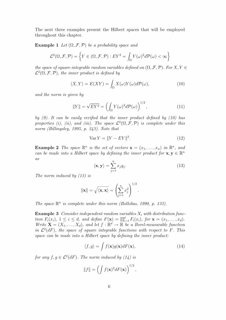
The next three examples present the Hilbert spaces that will be employedthroughout this chapter.

Example 1 Let (Ω,F ,P) be a probability space and

L2(Ω,F ,P) =Y ∈ (Ω,F ,P) : EY 2 =

∫

ΩY (ω)2dP(ω) < ∞

the space of square-integrable random variables defined on (Ω,F ,P). For X,Y ∈L2(Ω,F ,P), the inner product is defined by

〈X,Y 〉 = E(XY ) =∫

ΩX(ω)Y (ω)dP(ω), (10)

and the norm is given by

‖Y ‖ =√

EY 2 =(∫

ΩY (ω)2dP(ω)

)1/2

, (11)

by (9). It can be easily verified that the inner product defined by (10) hasproperties (i), (ii), and (iii). The space L2(Ω,F ,P) is complete under thisnorm (Billingsley, 1995, p. 243). Note that

Var Y = ‖Y − EY ‖2. (12)

Example 2 The space Rn is the set of vectors x = (x1, . . . , xn) in Rn, andcan be made into a Hilbert space by defining the inner product for x,y ∈ Rn

as

〈x,y〉 =n∑

j=1

xjyj. (13)

The norm induced by (13) is

‖x‖ =√〈x,x〉 =

n∑

j=1

x2j

1/2

.

The space Rn is complete under this norm (Bollobas, 1990, p. 133).

Example 3 Consider independent random variables Xi with distribution func-tion Fi(xi), 1 ≤ i ≤ d, and define F (x) =

∏di=1 Fi(xi), for x = (x1, . . . , xd).

Write X = (X1, . . . , Xd), and let f : Rd → R be a Borel-measurable functionin L2(dF ), the space of square integrable functions with respect to F . Thisspace can be made into a Hilbert space by defining the inner product:

〈f, g〉 =∫

f(x)g(x)dF (x), (14)

for any f, g ∈ L2(dF ). The norm induced by (14) is

‖f‖ =(∫

f(x)2dF (x))1/2

,

6

and L2(dF ) is complete under this norm (Billingsley, 1995, p. 243).

The notion of orthogonality among elements lies at the heart of Hilbert spacetheory, and extends the notion of perpendicularity in Euclidean space. Twoelements x, y are orthogonal if

〈x, y〉 = 0.

From here, there is just one step to the Pythagorean theorem:

Result 1 (Pythagorean Theorem) Kreyszig (1978). If x1, . . . , xn are pairwiseorthogonal vectors of an inner product space V then

∥∥∥∥∥n∑

i=1

xi

∥∥∥∥∥2

=n∑

i=1

‖xi‖2. (15)

Let us write

x⊥ = y ∈ V : 〈x, y〉 = 0for the set of orthogonal vectors to x ∈ V , and

S⊥ = y ∈ V : 〈x, y〉 = 0, ∀x ∈ S

for S ⊂ V . Finally, a set (x1, . . . , xn) of elements in V is orthogonal if all itselements are pairwise orthogonal.

We often work with a subspace S of a Hilbert space H defined on X, by whichwe mean a vector subspace of X with the inner product restricted to S × S.It is important to know when S is complete, and therefore a Hilbert space. Itis easy to prove that S is complete if and only if S is closed in H.

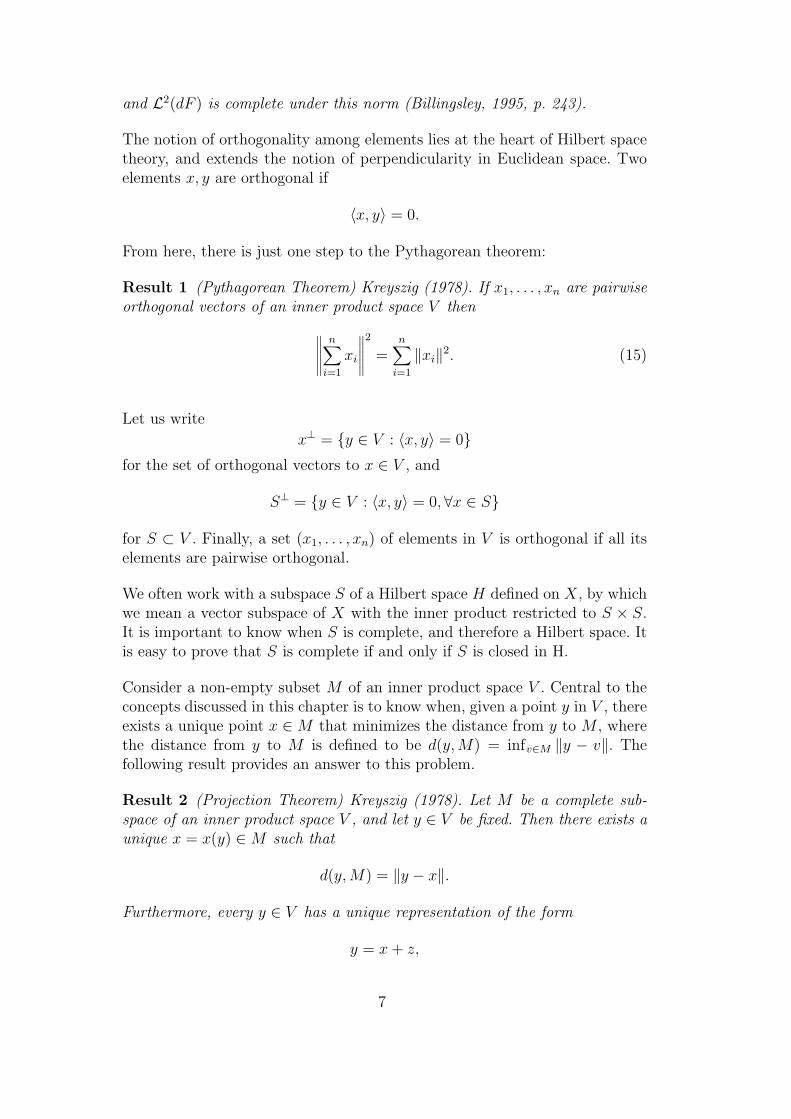
Consider a non-empty subset M of an inner product space V . Central to theconcepts discussed in this chapter is to know when, given a point y in V , thereexists a unique point x ∈ M that minimizes the distance from y to M , wherethe distance from y to M is defined to be d(y,M) = infv∈M ‖y − v‖. Thefollowing result provides an answer to this problem.

Result 2 (Projection Theorem) Kreyszig (1978). Let M be a complete sub-space of an inner product space V , and let y ∈ V be fixed. Then there exists aunique x = x(y) ∈ M such that

d(y,M) = ‖y − x‖.

Furthermore, every y ∈ V has a unique representation of the form

y = x + z,

7

¡¡

¡¡

¡¡

¡¡

¡¡

¡¡µ

-

­­

­­

­­

­­­

­­

­­

­­

­­­

6

y

PMy = x

(I − PM)y = z

M

Fig. 1. Orthogonal Projection

where x ∈ M and z ∈ M⊥. Then

〈x, y − x〉 = 〈x, z〉 = 0. (16)

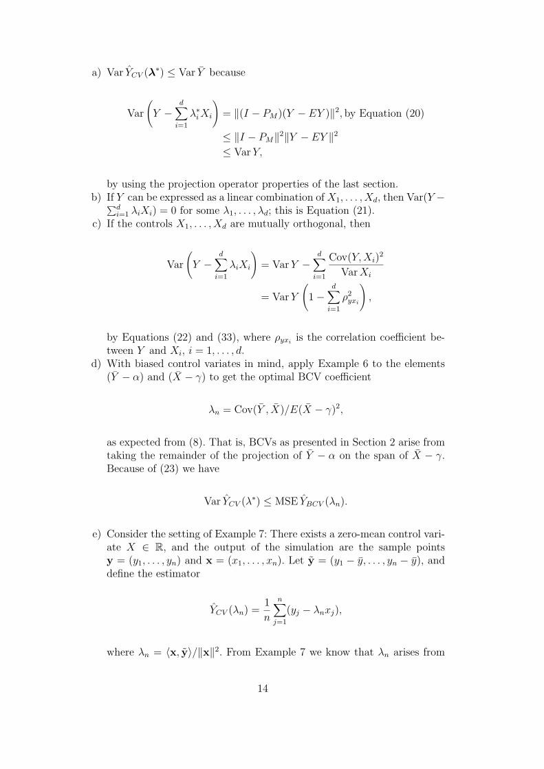
The second part of Result 2 implies that if M is a complete subspace of aninner product space V , then there exists a function PM : V → M defined byPMy = x. We call PM the orthogonal projection of V onto M , see Figure 1.

Among the properties that the projection functional enjoys are:

a) PMx = x, for all x ∈ M .b) PMz = 0, for all z ∈ M⊥.c) ‖I − PM‖ ≤ 1.

Applying Result 2 to Examples 1, 2, and 3 leads to several variance reductiontechniques in the Hilbert space setting. The following example forms the basisfor the method of conditional Monte Carlo.

Example 4 In the setting of Example 1, consider a sub-σ-algebra G of F . Theset of square integrable random variables defined on L2(Ω,G,P) is a completesubspace of L2(Ω,F ,P). Therefore, for Y ∈ L2(Ω,F ,P) fixed, there exists anelement Z ∈ L2(Ω,G,P) that is the closest point to Y in L2(Ω,G,P) and forwhich

〈Y − Z,W 〉 = 0, (17)

for W ∈ L2(Ω,G,P) arbitrary. Choosing W = IB, B ∈ G, Equation (17)shows that Z is the conditional expectation of Y given G, Z = E(Y |G). Wealso can write PGY = E(Y |G); see Williams (1991) for more details.

Observe that Equation (17) and the Pythagorean theorem imply that

‖Y ‖2 = ‖Y − Z‖2 + ‖Z‖2. (18)

8

Using Equation (12), centering Y so that EY = 0, we have that Equation (18)is the variance decomposition formula (Law and Kelton, 2000):

Var Y = E Var(Y |G) + Var E(Y |G), (19)

where Var(Y |G) = E(Y 2|G)− (E(Y |G))2.

We continue with an example with a view towards control variates.

Example 5 For elements X1, . . . , Xd ∈ L2(Ω,F ,P) with zero mean (oth-erwise re-define Xi := Xi − EXi), define M = Z ∈ L2(Ω,F ,P) : Z =∑d

i=1 βiXi, for all βi ∈ R, i = 1, . . . , d. For Y ∈ L2(Ω,F ,P), Result 2 thenguarantees the existence of constants β∗1 = β∗1(Y ), . . . , β∗d = β∗d(Y ) such that,

PM(Y −EY ) =d∑

i=1

β∗i Xi, and (I−PM)(Y −EY ) = (Y −EY )−d∑

i=1

β∗i Xi. (20)

If Y − EY ∈ M , using property a) of the projection operator we obtain (I −PM)(Y − EY ) = 0, so that

Var

(Y −

d∑

i=1

β∗i Xi

)= 0. (21)

If the elements X1, . . . , Xd form an orthogonal set, applying Equation (15) wehave

‖(I − PM)(Y − EY )‖2 = ‖Y − EY ‖2 − ‖PM(Y − EY )‖2

= ‖Y − EY ‖2 −d∑

i=1

β∗2i ‖Xi‖2,

so that

Var

(Y −

d∑

i=1

β∗i Xi

)= Var Y −

d∑

i=1

β∗2i Var Xi. (22)

When the elements X1, . . . , Xd are not mutually orthogonal but linearly inde-pendent, the Gram-Schmidt process (Billingsley, 1995, p. 249) yields an or-thogonal set with the same span as X1, . . . , Xd. In case the Xi’s are linearlydependent, at least one Xi can be expressed as a linear combination of the oth-ers, and eliminated from the set X1, . . . , Xd. By noticing that Cov(Xi, Xj) =〈Xi, Xj〉 we gather that X1, . . . , Xd are linearly independent if and only if theircovariance matrix is non-singular, and X1, . . . , Xd are mutually orthogonal ifand only if their covariance matrix has all its entries equal to zero except forpositive numbers on the diagonal.

We can extend Example 5 to the setting of biased control variates.

9

Example 6 Let X ∈ L2(Ω,F ,P), and M = Z ∈ L2(Ω,F ,P) : Z = β(X −γ),∀β ∈ R, γ 6= EX. Fix an element Y ∈ L2(Ω,F ,P) and let α = EY .Project Y − α on M :

PM(Y − α) = β∗(X − γ), and (I − PM)(Y − α) = Y − α− β∗(X − γ),

for some β∗ = β∗(Y ) ∈ R. As in the last example we have

‖(I − PM)(Y − α)‖2 = ‖Y − α‖2 − ‖PM(Y − α)‖2

and, since 〈(I − PM)(Y − α), X − γ〉 = 0, it follows that

β∗ =〈Y − α,X − γ〉‖X − γ‖2

.

The Pythagorean theorem applied to the denominator in the last equation yields

‖X − γ‖2 = ‖X − EX‖2 + ‖EX − γ‖2, (23)

which is known as the bias-variance decomposition formula.

The following example is geared to the method of control variates when theoptimal control coefficient is estimated from the sample data.

Example 7 Let x = (x1, . . . , xn) and y = (y1, . . . , yn) be elements of Rn (cf.Example 2), and define S = z ∈ Rn : z = βx, ∀β ∈ R. By Result 2 we have

PSy = βnx, and (I − PS)y = y − βnx,

for some βn = βn(y). Because 〈y − βnx,x〉 = 0, for ‖x‖ > 0,

βn =〈x,y〉‖x‖2

.

We now set the stage for the method of Latin hypercube sampling.

Example 8 Building on Example 3, let M = h ∈ L2(dF ) : h(x) =∑d

i=1 hi(xi)be the subspace of L2(dF ) spanned by the linear combinations of univariatefunctions h1, . . . , hd. Because M is complete, appealing to Result 2 establishesthe existence of an element h∗ = h∗(f) ∈ M , h∗(x) =

∑di=1 h∗i (xi), such that

‖f − h∗‖ = infh∈M ‖f − h‖ for f ∈ L2(dF ) fixed, and of a projection oper-ator PM : PMf = h∗. Similarly, for Mi = h ∈ L2(dF ) : h(x) = hi(xi),1 ≤ i ≤ d, there exists g∗i = g∗i (f) ∈ Mi: ‖f − g∗i ‖ = infh∈Mi

‖f − h‖ anda projection Pi : Pif = g∗i . To complete the picture, define the subspaceM0 = β ∈ R : |β| < ∞ which induces the projection P0 : P0f = g∗0, forg∗0 : ‖f − g∗0‖ = infβ∈M0 ‖f − β‖. We now have:

10

- Let Fi = σ(R × R × · · · × R × B × R × · · · × R : B ∈ B), where Bis the Borel σ−field, and let F0 be the trivial σ-algebra ∅,R. For eachPi, we know that 〈f − Pif, h〉 = 0 for any h ∈ Mi; choosing h(x) =hi(xi) = IB(xi), B ∈ B, shows that Pif = E(f(X)|Fi) for 1 ≤ i ≤ d, andP0f = E(f(X)|F0) = Ef(X).

- Suppose P0f = 0. Then (I − PM)f ∈ M⊥i implies g∗i = Pif = PiPMf =

h∗i , which results in

PM =d∑

i=1

Pi, and PMf =d∑

i=1

E(f(X)|Fi). (24)

For general P0f 6= 0, (24) becomes

PM = P0 +d∑

i=1

(Pi−P0), and PMf = Ef(X)+d∑

i=1

(E(f(X)|Fi)−Ef(X)).

(25)

The next result, a variant of Result 2, will be useful when we consider themethod of weighted Monte Carlo.

Result 3 Kreyszig (1978) Suppose M 6= ∅ is a closed convex subset of aHilbert space H. Then for x ∈ H fixed, x1 = PM(x) is the (unique) closestpoint in M to x if and only if

〈x− x1, y − x1〉 ≤ 0,∀y ∈ M. (26)

Later in the chapter we will deal with sequences of projections, say (Pn),defined on a Hilbert space H that are monotone increasing in that

‖Pix‖ ≤ ‖Pi+1x‖, for i = 1, 2, . . . ,

and x ∈ H arbitrary. Using the completeness of H it can be shown that (Pn)converges in the following sense:

Result 4 Kreyszig (1978) Let (Pn) be a monotone increasing sequence of pro-jections Pn defined on a Hilbert space H. Then, for any x ∈ H,

‖Pnx− Px‖ → 0,

and the limit operator P is a projection on H.

An immediate application of this result is the following example.

Example 9 Suppose that (Fn) is an increasing sequence F1 ⊆ F2 ⊆ . . . ⊆F∞ of σ-algebras such that F∞ = σ(∪∞n=1Fn). Then associated with everyL2(Ω,Fn,P) there exists a projection Pn : L2(Ω,F ,P) → L2(Ω,Fn,P), and

11

the sequence of projections (Pn) is monotone increasing. Let P∞ be the pro-jection that results from applying Result 4: ‖PnW − P∞W‖ → 0 for anyW ∈ L2(Ω,F ,P), F∞ ⊆ F . Because (I − P∞)W ∈ L2(Ω,Fn,P)⊥, we have

∫

BWdP =

∫

BP∞WdP (27)

for any B ∈ Fn. A standard π−λ argument (Durrett, 1996, p. 263) shows that(27) holds for B ∈ F∞ arbitrary; that is, P∞W = E(W |F∞). The conclusionis

‖E(W |F∞)− E(W |Fn)‖ → 0, (28)

as n →∞.

We will appeal to Example 9 when dealing with stratification techniques. Avariation of the last example is

Example 10 Suppose that X is random variable with known and finite mo-ments EX i, i = 1, 2, . . .. Define a sequence of complete subspaces (Md) ofL2(Ω, σ(X),P) by

Md =

Z ∈ L2(Ω, σ(X),P) : Z =

d∑

i=1

βi(Xi − EX i),∀βi ∈ R, 1 ≤ i ≤ d

,

for d = 1, 2, . . .. Clearly M1 ⊆ M2 ⊆ . . . ⊆ M∞, where M∞ = ∪∞i=1Mi.Associated with each Md there is, by Result 2, a projection operator Pd withrange on Md such that for W ∈ L2(Ω,F ,P), σ(X) ⊆ F , with EW = 0:

PdW =d∑

i=1

β∗i (Xi − EX i), (29)

for some constants β∗i = β∗i (W ), 1 ≤ i ≤ d, possibly dependent on d (althoughthis is not apparent from the notation). Because the sequence of operators (Pd)is (clearly) monotone increasing, Result 4 ensures the existence of a projectionP∞ in L2(Ω, σ(X),P) that satisfies

‖P∞W − PdW‖ → 0, (30)

as d →∞. Proceeding like in the last example it follows that P∞W = E(W |X),for W ∈ L2(Ω,F ,P) arbitrary. In other words,

∥∥∥∥∥E(W |X)−d∑

i=1

β∗i (Xi − EX i)

∥∥∥∥∥ → 0, (31)

as d →∞, by Equations (29) and (30).

We will use the last example in Section 6 to show how conditional Monte Carloand control variates reduce variance cooperatively.

12

The rest of the chapter is devoted to provide an interpretation of this section’sexamples in terms of variance reduction techniques. We start with the methodof control variates.

4 A Hilbert Space Approach to Control Variates

We build on the sequence of examples from the previous section; Glynn andSzechtman (2002) is a relevant reference for the issues discussed in this section.

Consider the setting of Example 5: X1, . . . , Xd are zero-mean square integrablerandom variables with non-singular covariance matrix Σxx (although this wasnot needed in Example 5), and defined on the same probability space as theresponse Y , EY 2 < ∞. The goal is to estimate α = EY by averaging ni.i.d. replicates of Y −∑d

i=1 λiXi to obtain YCV (λ) as in Equation (1). Clearly,Var YCV (λ) = 1/n Var(Y −∑d

i=1 λiXi).

From Example 5, YCV (λ∗) is the remainder from projecting Y on M ; asM “grows” the norm of the remainder decreases. Also, because the scalarsλ∗1, . . . , λ

∗d that minimize Var(Y −∑d

i=1 λiXi) are also the numbers that resultfrom projecting Y into M , from Result 2 and Equation (16) we know that

〈Y −d∑

i=1

λ∗i Xi, Z〉 = 0, ∀Z ∈ M.

In particular,

〈Y −d∑

i=1

λ∗i Xi, λ∗kXk〉 = 0, for k = 1, . . . , d. (32)

Therefore, since Cov(Y, Xj) = 〈Y, Xj〉, and Cov(Xi, Xj) = 〈Xi, Xj〉 for 1 ≤i, j ≤ d,

λ∗i = (Σ−1xxΣxy)i, for i = 1, . . . , d,

in concordance with Equation (3). When X1, . . . , Xd is an orthogonal set,Equation (32) yields

λ∗i =〈Y,Xi〉〈Xi, Xi〉 =

Cov(Y,Xi)

Var Xi

, i = 1, . . . , d. (33)

We re-interpret the results from Examples 5 through 7 in the CV context:

13

a) Var YCV (λ∗) ≤ Var Y because

Var

(Y −

d∑

i=1

λ∗i Xi

)= ‖(I − PM)(Y − EY )‖2, by Equation (20)

≤ ‖I − PM‖2‖Y − EY ‖2

≤ Var Y,

by using the projection operator properties of the last section.b) If Y can be expressed as a linear combination of X1, . . . , Xd, then Var(Y −∑d

i=1 λiXi) = 0 for some λ1, . . . , λd; this is Equation (21).c) If the controls X1, . . . , Xd are mutually orthogonal, then

Var

(Y −

d∑

i=1

λiXi

)= Var Y −

d∑

i=1

Cov(Y,Xi)2

Var Xi

= Var Y

(1−

d∑

i=1

ρ2yxi

),

by Equations (22) and (33), where ρyxiis the correlation coefficient be-

tween Y and Xi, i = 1, . . . , d.d) With biased control variates in mind, apply Example 6 to the elements

(Y − α) and (X − γ) to get the optimal BCV coefficient

λn = Cov(Y , X)/E(X − γ)2,

as expected from (8). That is, BCVs as presented in Section 2 arise fromtaking the remainder of the projection of Y − α on the span of X − γ.Because of (23) we have

Var YCV (λ∗) ≤ MSE YBCV (λn).

e) Consider the setting of Example 7: There exists a zero-mean control vari-ate X ∈ R, and the output of the simulation are the sample pointsy = (y1, . . . , yn) and x = (x1, . . . , xn). Let y = (y1 − y, . . . , yn − y), anddefine the estimator

YCV (λn) =1

n

n∑

j=1

(yj − λnxj),

where λn = 〈x, y〉/‖x‖2. From Example 7 we know that λn arises from

14

projecting y on the span of x: PSy = λnx. Now, the sample variance is

1

n

n∑

j=1

(yj − λnxj − YCV (λn))2 =1

n‖(I − PS)y‖2 − (YCV (λn)− y)2

=1

n(‖y‖2 − λ2

n‖x‖2) + O(n−1)

=1

n‖y‖2(1− ρ2

y,x) + O(n−1),

where ρy,x = 〈x, y〉/‖x‖‖y‖, which makes precise the variance reductionachieved by projecting y on the span of x relative to the crude estimatorsample variance ‖y‖2/n.

Finally, we remark that there is no impediment in extending items a) throughe) to the multi-response setting, where Y is a random vector.

5 Conditional Monte Carlo in Hilbert Space

In this section we address the method of conditional Monte Carlo, payingspecial attention to its connection with control variates; we follow Avramidisand Wilson (1996), and Loh (1995).

Suppose Y ∈ L2(Ω,F ,P) and that we wish to compute α = EY . Let X ∈L2(Ω,F ,P) be such that E(Y |X) can be analytically or numerically com-puted. Then

YCMC =1

n

n∑

j=1

E(Y |Xi)

is an unbiased estimator of α, where the E(Y |Xi) are found by first obtainingi.i.d. samples Xi and then computing E(Y |Xi). We call YCMC the conditionalMonte Carlo (CMC) estimator of α; remember that according to Example 4,YCMC results by projecting Y on L2(Ω, σ(X),P). The variability of YCMC isgiven by

Var YCMC =1

nVar E(Y |X),

with Equation (19) implying that Var YCMC ≤ Var Y . Specifically, CMC elim-inates the E Var(Y |X) term from the variance of Y .

Sampling from Y − λ(Y −E(Y |X)) also provides an unbiased estimator of α

15

for any λ ∈ R. By Equation (3),

λ∗ =〈Y, (I − Pσ(X))Y 〉‖(I − Pσ(X))Y ‖2

=〈Pσ(X)Y + (I − Pσ(X))Y, (I − Pσ(X))Y 〉

‖(I − Pσ(X))Y ‖2

= 1.

(34)

This shows that CMC is optimal from a CV perspective. Avramidis and Wil-son (1996), and Loh (1995), generalize this approach: Let Z be a zero-meanrandom variable in L2(Ω,F ,P), and X a random variable in L2(Ω,F ,P) forwhich both E(Y |X) and E(Z|X) can be determined. Then sampling from

Y − λ1(Y − E(Y |X))− λ2E(Z|X)− λ3Z (35)

can be used to form the standard means based estimator for α, for all λ1, λ2, λ3 ∈R. Repeating the logic leading to (34) we obtain

λ∗1 = 1, λ∗2 =Cov(E(Y |X), E(Z|X))

Var E(Z|X), and λ∗3 = 0.

The conclusion is that,

Var

(E(Y |X)− Cov(E(Y |X), E(Z|X))

Var E(Z|X)E(Z|X)

)

≤

Var Y,

Var E(Y |X),

Var(Y − Cov(Y,Z)

Var ZZ

),

Var(Y − Cov(Y,E(Z|X))

Var E(Z|X)E(Z|X)

),

Var(E(Y |X)− Cov(E(Y |X),Z)

Var ZZ

).

In particular, Loh (1995) considers the case of Z = X almost surely in (35),and Avramidis and Wilson (1996) fix λ1 = 1 and λ3 = 0 in (35). From thenorm perspective,

‖E(Y |X)− α− λ∗2E(Z|X)‖2 = ‖Y − α‖2 − ‖Y − E(Y |X)‖2 − ‖λ∗2E(Z|X)‖2

makes precise the variance eliminated when sampling from E(Y |X)−λ∗2E(Z|X).

16

6 Control Variates and Conditional Monte Carlo from a HilbertSpace Perspective

We now discuss how CMC and CV can be combined to reduce variance co-operatively; the results of this section appear in Loh (1995), and Glynn andSzechtman (2002).

Suppose the setting of Example 10: There exists a random variable X ∈L2(Ω,F ,P) such that the moments EX i are known with E|X|i < ∞ for alli = 1, 2, . . .. Given a random variable Y ∈ L2(Ω,F ,P), the goal is to findα = EY by running a Monte Carlo simulation that uses the knowledge aboutthe moments of X to increase simulation efficiency. Suppose we can samplefrom either

a) E(Y |X)−∑di=1 λ∗i (X

i − EX i)

or

b) Y −∑di=1 λ∗i (X

i − EX i),

to form the standard estimator for α, where the λ∗i are determined by applyingEquation (3) on E(Y |X) and on the controls (X1−EX1, . . . , Xd−EXd). Fromthe developments of Example 10 it is a short step to:

a) Take W = E(Y |X)− α in Equation (31), consequently:

Var

(E(Y |X)−

d∑

i=1

λ∗i (Xi − EX i)

)→ 0, (36)

as d →∞.b) The triangle inequality and W = Y − α in Equation (31) result in

Var

(Y −

d∑

i=1

λ∗i (Xi − EX i)

)→ E Var(Y |X), (37)

as d →∞.

The interpretation of a) is that CV and CMC reduce variance concurrently:E(Y |X) eliminates the E Var(Y |X) part of Var Y , while

∑di=1 λ∗i (X

i − EX i)asymptotically cancels Var E(Y |X). The effect of

∑di=1 λ∗i (X

i − EX i) in partb) is to asymptotically eliminate the variance component due to E(Y |X) whenusing E(Y |X) in the simulation is not possible.

17

7 Weighted Monte Carlo

In this section we consider the asymptotic behavior of weighted Monte Carlo(WMC) estimators, for a large class of objective functions. We rely on Glasser-man and Yu (2005), and Glasserman (2004), which make precise the connec-tion between WMC and CVs for separable convex objective functions. Initialresults, under weaker assumptions and just for one class of objectives were ob-tained in Szechtman and Glynn (2001), and in Glynn and Szechtman (2002).Applications of weighted estimators to model calibration in the finance con-text are presented in Avellaneda et al. (2001), and in Avellaneda and Gamba(2000).

Consider the standard CV setting: (Y1,X1), . . . , (Yn,Xn) are i.i.d. samplesof jointly distributed random elements (Y,X) ∈ (R,Rd) with non-singularcovariance matrix Σ and, without loss of generality, EX = 0 componentwise.The goal is to compute α = EY by Monte Carlo simulation, using informationabout the means EX to reduce estimator variance. Let f : R→ R be a strictlyconvex and continuously differentiable function, and suppose that the weightsw∗

1,n, . . . , w∗n,n

minimizen∑

k=1

f(wk,n) (38)

subject to1

n

n∑

k=1

wk,n = 1 (39)

1

n

n∑

k=1

wk,nXk = 0. (40)

Then, the WMC estimator of α takes the form

YWMC =1

n

n∑

k=1

w∗k,nYk.

The following observations review some key properties of WMC: The weightapplied to each replication i is w∗

i,n/n, rather than the weight 1/n used to form

the sample mean Y . A feasible set of weights is one that makes YWMC unbi-ased (cf. constraint (39)), and that forces the weighted average of the controlsamples to match their known mean (cf. constraint (40)). For every n suffi-ciently large 0 (=EX) belongs to the convex hull of the replicates X1, . . . ,Xn,and therefore the constraint set is non-empty. The objective function in (38),being strictly convex, ensures uniqueness of the optimal solution if the optimalsolution is finite. If wk,n ≥ 0, 1 ≤ k ≤ n, were additional constraints, a feasi-ble set of weights w1,n, . . . , wn,n would determine a probability mass function1/n

∑nk=1 δXk

(·)wk,n, where δx(z) = 1 if z = x and is equal to zero otherwise.However, as discussed in Hesterberg and Nelson (1998), P (wk,n < 0) = o(n−p)

18

uniformly in 1 ≤ k ≤ n if E(‖X‖p) < ∞ indicates that the non-negativityconstraints are asymptotically not binding; see Szechtman and Glynn (2001)for an example of this scenario.

There are different f ’s depending on the application setting. For example:f(w) = − log w results in maximizing empirical likelihood; discussed in Szecht-man and Glynn (2001). The function f(w) = −w log w yields an entropy max-imization objective; this is the subject of Avellaneda and Gamba (2000), andAvellaneda et al. (2001). The important case of f(w) = w2 is considered next,the optimization problem being to

minimizen∑

k=1

w2k,n

subject to1

n

n∑

k=1

wk,n = 1 (41)

1

n

n∑

k=1

wk,nXk = 0.

Solving the optimization problem yields (Glasserman and Yu, 2005) optimalweights given by

w∗k,n = 1− XTM−1(Xk − X), for k = 1, . . . , n, (42)

where M ∈ Rd×d is the matrix with elements Mi,j = 1/n∑n

k=1(Xi,k−X)(Xj,k−X); M−1 exists for all n large enough because M → Σxx a.s. componentwise.Rearranging terms immediately gives

1

n

n∑

k=1

w∗k,nYk = YCV (λn), (43)

with the benefit that the optimal weights do not depend on the Yk, whichmakes this approach advantageous when using CVs for quantile estimation;see Hesterberg and Nelson (1998) for details.

Regarding Hilbert spaces, consider the space Rn (cf. Example 2) and the set

A(n) =

w(n) = (w1,n, . . . , wn,n) ∈ Rn :

1

n

n∑

k=1

wk,n = 1 and1

n

n∑

k=1

wk,nXk = 0

.

It can be verified that A(n) meets the conditions of Result 3 for every n suffi-ciently large, and consequently it is fair to ask: What element in A(n) is closestto 1(n) = (1, . . . , 1) ∈ Rn? That is, which element w∗(n) = (w∗

1,n, . . . , w∗n,n) ∈

Rn

minimizes ‖1(n)−w(n)‖subject to w(n) ∈ A(n)?

19

This problem yields the same solution as problem (41); doing simple algebrait is easy to verify that w∗(n) with components as in Equation (42) satisfiescondition (26). The conclusion is that w∗(n) is the closest point in A(n) to1(n), the vector of crude sample weights. Would this Hilbert space approachto WMC work with f ’s that are not quadratic? Yes, as long as the metricinduced by the inner product meets the defining properties of a metric.

The main result concerning WMC and CV, proved in Glasserman and Yu(2005) under certain conditions on X, Y , f , and the Lagrange multipliersassociated with constraints (39) and (40), is that

YWMC = YCV + Op(n−1),

and, √n(YWMC − α) ⇒ N(0, σ2

WMC),

as n →∞ whereσ2

WMC = σ2CV ,

and Op(an) stands for a sequence of random variables (ξn : n ≥ 1) such thatfor all ε > 0 and some constant δ, P (|ξn| ≥ anδ) < ε. The last result providessupport to the statement that YWMC and YCV are asymptotically identical.

8 Stratification Techniques

In this section we discuss stratification methods emphasizing the connectionwith the Hilbert space and CVs ideas already developed. Refer to Fishman(1996), Glasserman et al. (1999), and Glynn and Szechtman (2002) for moredetails.

Suppose that we wish to compute α = EY , for some random variable Y ∈L2(Ω,F ,P). Let X ∈ L2(Ω,F ,P). The method of stratification arises whenthere is a collection of disjoint sets (“strata”) (Ai : 1 ≤ i ≤ d) in the range ofX such that P (X ∈ ∪d

i=1Ai) = 1 and P (X ∈ Ai) = pi is known for every 1 ≤i ≤ d. Then, assuming that one can obtain i.i.d. replicates (Yi,k : 1 ≤ k ≤ ni)from P (Y ∈ ·|X ∈ Ai), 1 ≤ i ≤ d, the estimator of α given by

d∑

i=1

pi

ni

ni∑

k=1

Yi,k (44)

is unbiased, where ni is the number of replicates sampled from P (Y ∈ ·|X ∈Ai).

For a total number of replications n =∑d

i=1 ni, proportional stratificationallocates ni = npi samples to strata Ai, 1 ≤ i ≤ d, where for simplicity we

20

assume that the npi are integers. The estimator of Equation (44) is then calledthe proportional stratification (PS) estimator

YPS =1

n

d∑

i=1

npi∑

k=1

Yi,k,

with variance given by

Var YPS =1

n

d∑

i=1

pi Var(Y |Z = i)

=1

nE Var(Y |Z),

(45)

where the random variable Z =∑d

i=1 iI(X ∈ Ai).

One implication of Equation (45) is that if Y is not constant inside eachstrata, then Var YPS > 0, so that proportional stratification does not eliminatethe variability of Y inside strata, but rather the variability of E(Y |Z) acrossstrata. In addition, Equation (45), jointly with the variance decompositionformula (19), quantifies the per-replication variance reduction achieved byproportional stratification: E Var(Y |Z) = Var Y − Var E(Y |Z). Observe thatalthough PS is relatively simple to implement, it does not provide the optimalsample allocation ni per strata; see Glasserman (2004, p. 217) for more details.

From a CV perspective, PS acts like applying E(Y |Z) − α as a CV on Y ;YPS achieves the same variance reduction as that obtained by averaging i.i.d.replications of Y − (E(Y |Z) − α). Of course, sampling from the distributionof Y − (E(Y |Z)− α) is impractical because α is unknown.

Regarding Hilbert spaces, Equation (45) is simply

n Var YPS = ‖(I − Pσ(Z))Y ‖2. (46)

In addition, YPS satisfies the following CLT:

n1/2(YPS − α) ⇒ N(0, σ2PS) as n →∞,

where σ2PS = E Var(Y |Z), which enables the construction of asymptotically

valid confidence intervals for α.

Post-stratification offers an alternative to proportional stratification whensampling from P (Y ∈ ·|X ∈ Ai) is not possible, but when it is possible tosample from the distribution of (X, Y ). Specifically, we construct the unbiasedestimator

YpST =d∑

i=1

pi

∑nk=1 YkI(Xk ∈ Ai)∑n

j=1 I(Xj ∈ Ai).

21

Using the Delta method (cf. Section 2) it is easy to prove a CLT for YpST :

n1/2(YpST − α) ⇒ N(0, σ2pST ),

as n → ∞, where σ2pST = E Var(Y |Z). However, for every stratum we know

a priori that EI(X ∈ Ai) = pi, which suggests the use of the vector (I(X ∈Ai)− pi : 1 ≤ i ≤ d) as a control. More specifically, an unbiased CV estimatoris given by

YCV (λ) =1

n

n∑

j=1

(Yj −

d∑

i=1

λi(I(Xj ∈ Ai)− pi)

).

Using Equation (3), the optimal coefficients λ∗i , 1 ≤ i ≤ d are immediatelyfound to be

λ∗i = E(Y |Z = i), for 1 ≤ i ≤ d.

That is,

YCV (λ∗) =1

n

n∑

j=1

(Yj − (E(Y |Zj)− α)) ,

and

Var YCV (λ∗) =1

nE Var(Y |Z).

Therefore, n(Var YCV (λ∗) − Var YpST ) → 0 as n → ∞. With a little moreeffort, it can be shown that

n1/2(YpST − YCV (λ∗)

)⇒ 0,

as n → ∞. In other words, YpST and YCV (λ∗) have the same distribution upto an error of order op(n

−1/2), as n →∞; where op(an) denotes a sequence ofrandom variables (ξn : n ≥ 1) such that a−1

n ξn ⇒ 0 as n →∞.

Given the strata (Ai : 1 ≤ i ≤ d), it is always possible to find finer strata thatfurther reduce estimator variance. In the case of proportional stratification,suppose that it is possible to split each stratum Ai into integer ni = npi strata(Ai,k : 1 ≤ k ≤ ni) such that P (X ∈ Ai,k) = 1/n; i.e., the bivariate randomvector Vn =

∑di=1

∑nik=1(i, k)I(X ∈ Ai,k) is uniformly distributed on the lattice

(i, k) : 1 ≤ i ≤ d, 1 ≤ k ≤ ni. Assume in addition that it is possible tosample from P (Y ∈ ·|X ∈ Ai,k). Then the refined proportional stratification(rST) estimator is

YrST =1

n

d∑

i=1

npi∑

k=1

Yi,k,

where the Yi,k are sampled from P (Y ∈ ·|X ∈ Ai,k). Proceeding as in (45), wearrive at

Var YrST =1

nE Var(Y |Vn).

22

The fact that ‖E(Y |Vn)−EY ‖2 = ‖E(Y |Vn)−E(Y |Z)‖2 + ‖E(Y |Z)−EY ‖2

shows that Var E(Y |Vn) ≥ Var E(Y |Z), and therefore

Var YrST ≤ Var YPS.

With regards to Example 9, the conditions leading to Equation (28) apply, sothat as n →∞

Var(E(Y |X)− E(Y |Vn)) → 0,

and

Var(Y − E(Y |Vn)) → E Var(Y |X).

In particular, n Var YrST → E Var(Y |X). This result should come as no sur-prise because as n grows we get to know the full distribution of X, not unlikethe setting of Equations (36) – (37): rST presumes knowledge of an increasingsequence of σ-algebras that converge to σ(X), whereas in Equations (36) –(37) we have information about the full sequence of moments of X.

As to control variates, rST produces the same estimator variance as the stan-dard CV estimator formed by i.i.d. sampling from Y − (E(Y |X) − α), asn → ∞. Similar to (46), we can write n Var YrST → ‖(I − Pσ(X))Y ‖2, as

n →∞. Finally, the CLT satisfied by YrST is

n1/2(YrST − α) ⇒ N(0, σ2rST ),

as n →∞, where σ2rST = E Var(Y |X).

To conclude this section, we mention the link between post-stratification andWMC. Write

w∗k,n =

d∑

i=1

piI(Xk ∈ Ai)∑nj=1 I(Xj ∈ Ai)

, (47)

for 1 ≤ k ≤ n, then the WMC estimator YWMC =∑n

k=1 w∗k,nYk equals YpST . It

can be confirmed that the weights given in Equation (47) are the solution of theoptimization problem with objective function min

∑nk=1 w2

k,n and constraints∑nk=1 wk,nI(Xk ∈ Ai) = pi, 1 ≤ i ≤ d, and

∑nk=1 wk,n = 1. Interpreting at face

value, w∗n with elements as in (47) is the closest point in the set determined

by the constraints to the vector consisting of n ones.

9 Latin Hypercube Sampling

We now discuss the method of Latin hypercube sampling (LHS) from a Hilbertspace and CV perspective. McKay et al. (1979), Stein (1987), Owen (1992),and Loh (1996) are standard references for LHS. We rely on Mathe (2000),which gives a good account of LHS from a Hilbert space point of view.

23

Avramidis and Wilson (1996) is also a valuable reference for the issues weconsider.

Suppose the setting of Examples 3 and 8: We have mutually independentrandom variables X1, . . . , Xd, each with known distribution function Fi, andthe goal is to compute

α = Ef(X) =∫

f(x)dF (x)

via simulation, where f : Rd → R is a square integrable function with respectto F (x) =

∏nd=1 Fi(xi), x = (x1, . . . , xd), and X = (X1, . . . , Xd).

LHS generates samples of X as follows:

(i) Tile [0, 1)d into nd hypercubes ∆l1,...,ld =∏d

i=1[li−1

n, li

n), li = 1, . . . , n,

i = 1, . . . , d, each of volume n−d.(ii) Generate d uniform independent permutations (π1(·), . . . , πd(·)) of 1, . . . , n.(iii) Use the output of (ii) to choose n hypercubes from (i): ∆π1(k),...,πd(k) for

the k’th tile, k = 1, . . . , n.(iv) Uniformly select a point from within each ∆π1(k),...,πd(k), and generate Xi,k

by inverting Fi at that point.

Notice that (i) – (iv) are

Xi,k = F−1i

(πi(k)− 1 + Ui(k)

n

), 1 ≤ i ≤ d, and 1 ≤ k ≤ n, (48)

where the Ui(k) are i.i.d. uniform on [0, 1]. The LHS estimator is the averageof the n samples f(Xk), each Xk = (X1,k, . . . , Xd,k) obtained according to(48):

YLHS =1

n

n∑

k=1

f(Xk).

As in refined stratification, given a sample size n, LHS assigns one sample toeach strata Ai,k given by

Ai,k =

[F−1

i

(k − 1

n

), F−1

i

(k

n

)), 1 ≤ i ≤ d, 1 ≤ k ≤ n,

with the sample uniformly distributed within the strata. Where refined pro-portional stratification applied to a particular Xi asymptotically eliminatesthe variance due to E(f(X)|Fi) (cf. Example 8 for the definition of Fi) alongjust one dimension i, LHS asymptotically eliminates Var

∑di=1 E(f(X)|Fi) at

the same rate used by rST used to eliminate only Var E(f(X)|Fi).

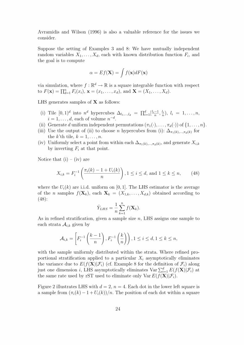
Figure 2 illustrates LHS with d = 2, n = 4. Each dot in the lower left square isa sample from (πi(k)− 1+Ui(k))/n. The position of each dot within a square

24

6

-

6

-

x1

F (x1)F (x2)

x2

££££££­

­­­

³³³³³³´´

´

©©©©©©

¢¢¢¢¢¢

r

r

r

r

r rrrX1,1 X1,4X1,3X1,2

r

rr

r

X2,1

X2,2

X2,3

X2,4

...

...

...

...

...

...

...

..

...

...

..

...

...

...

...

...

. . . . . . . . . . . . .

. . . . . . . . .

. . . . . . .

...

...

...

.

...

...

...

...

..

...

...

...

...

...

.... . . . . . . . . . . . . . . .

. . . . . . . . . . .. . . . .

A1,4A1,3A1,1A1,2

A2,4

A2,3

A2,1

A2,2

Fig. 2. Latin hypercube sampling

is uniformly distributed according to the Ui(k); the permutations πi(k) ensurethat there is just one dot per row and per column. The lower right regiondepicts F1 and the four equiprobable strata for X1, with one sample pointF−1

1 ((π1(k)− 1 + U1(k))/n) per strata A1,k; the final output are the samplesX1,1, . . . , X1,4. In the upper left F2 is pictured with the axes inverted; it hasthe same explanation as that of F1, with the final output being the samplesX2,1, . . . , X2,4.

Stein (1987) demonstrates that when f ∈ L2(dF ),

Var YLHS =1

nVar

(f(X)−

d∑

i=1

E(f(X)|Fi)

)+ o(n−1), (49)

as n → ∞, which makes precise the variance reduction achieved by LHS, upto order o(n−1).

The CLT satisfied by YLHS, proved in Owen (1992) under the condition thatf(F−1(·)) is bounded on [0, 1]d is

n1/2(YLHS − α) ⇒ N(0, σ2LHS), (50)

25

as n →∞, where

σ2LHS = Var

(f(X)−

d∑

i=1

E(f(X)|Fi)

).

Equation (50) provides theoretical support for the construction of a validconfidence interval for α, whose width depends on σLHS. This term is generallynot known prior to the simulation, nor easily estimated from the simulationdata. Section 3 of Owen (1992) deals with the estimation of σ2

LHS from LHSdata, and shows how to use the LHS samples to find an estimator for σ2

LHS

which is within n−1/2 in probability of σ2LHS as n → ∞. This permits the

formation of an asymptotically valid confidence interval for α.

As to standard Monte Carlo, Owen (1997) proves that LHS is no less efficientbecause

Var YLHS ≤ Var f(X)

n− 1,

for all n ≥ 2 and d ≥ 2. In other words, even if the variance eliminated by LHS,Var

∑di=1 E(f(X)|Fi), is small, LHS with n samples is no less efficient than

standard Monte Carlo with n− 1 replications. Of course, the only measure ofefficiency in this argument is variance, a more complete analysis would takeinto account the computational cost of generating sample variates.

Example 8 leads into the Hilbert interpretation of LHS. In particular, Equa-tions (25) and (49) imply

limn→∞n Var YLHS = Var

(f(X)−

d∑

i=1

E(f(X)|Fl)

)= ‖(I − PM)f‖2. (51)

That is, LHS takes the remainder from projecting f on the subspace M deter-mined by the span of the linear combinations of univariate functions. Usingthe last equation, LHS eliminates variance because

Var f(X) = ‖(I − P0)f‖2

= ‖PM(I − P0)f‖2 + ‖(I − PM)(I − P0)f‖2

≥ ‖(I − PM)(I − P0)f‖2

= ‖(I − PM)f‖2,

where

‖PM(I − P0)f‖2 =d∑

i=1

‖Pi(I − P0)f‖2 =d∑

i=1

Var E(f(X)|Fi)

is the variance eliminated by LHS. If f ∈ M , then Equation (51) also showsthat n Var YLHS → 0 as n →∞; in other words, LHS asymptotically eliminatesall the variance of f if f is a sum of univariate functions.

26

Much more can be said about Var f(X). Suppose for simplicity that the Xi areUniform [0, 1] random variables, so that α =

∫ 10 f(x)dx. Let u ⊆ 1, 2, . . . , d

and define dx−u =∏

j 6∈u dxj. Then, if f is square integrable, there is a uniquerecursion

fu(x) =∫

f(x)dx−u − ∑v⊂u

fv(x) (52)

with the property that∫ 10 fu(x)dxj = 0 for every j ∈ u, and

f(x) =∑

u⊆1,2,...,dfu(x);

see, for example, Jiang (2003) for a proof. Recursion (52) actually is the Gram-Schmidt process, and it splits f into 2d orthogonal components such that

∫fu(x)fv(x)dx = 0,

for u 6= v, andσ2 =

∑

|u|>0

σ2u, (53)

where σ2 =∫(f(x) − α)2dx is the variance of f(X), and σ2

u =∫

f 2u(x)dx is

the variance of fu(X). The conclusion in this context is that LHS eliminatesthe variance of the fu for all u with |u| = 1. The setting of this paragraph isknown as functional ANOVA; see Chapter 13 for more details on this topic.

Considering control variates, we can say that the estimator formed by averag-ing i.i.d. replicates of f(X)−∑d

i=1(E(f(X)|Fi)−α) has the same asymptoticvariance as YLHS. Moreover, given a zero-mean control variate h(X), h a de-terministic function, obtain n Latin hypercube samples of X using (48), andform the combined LHS+CV estimator

YLHS+CV (λ) =1

n

n∑

k=1

(f(Xk)− λh(Xk)) .

Then, n(Var YLHS+CV (λ)−Var YLHS) → 0 for any control of the type h(X) =∑di=1 hi(Xi) because h ∈ M and property a) of the projection operator together

imply (I − PM)(f − λh) = (I − PM)f for all λ ∈ R. Using Equations (4) and(49):

Var YLHS+CV (λ∗) = Var YLHS(1− ρ2),

where ρ2 is the square of the correlation coefficient between

f(X)−d∑

i=1

E(f(X)|Fi) and h(X)−d∑

i=1

E(h(X)|Fi).

In other words, a good CV for f(X) in the LHS context is one that maximizesthe absolute value of the correlation coefficient of its non-additive part withthe non-additive part of f(X). Notice that λ∗ is the optimal CV coefficient

27

associated with the response f(X) − ∑di=1 E(f(X)|Fi) and the CV h(X) −∑d

i=1 E(h(X)|Fi); refer to Owen (1992) for the estimation of λ∗ from sampledata.

Additional guidance for effective CVs in the LHS setting is provided by (53):Choose a CV with non-additive part that is highly correlated with fu’s, |u| > 1,that have σ2

u large.

As regards weighted Monte Carlo, consider using LHS to generate replicatesX1, . . . ,Xn, and the optimization problem

minimizen∑

k=1

w2k,n

subject ton∑

k=1

wk,n = 1 (54)

n∑

k=1

wk,nI(Xi,k ∈ Ai,j) =1

n, for i = 1, . . . , d and j = 1, . . . , n.

Clearly w∗k,n = 1/n, k = 1, . . . , n, is feasible for (54), and it is also optimal by

the developments of Section 7, so that the WMC estimator∑n

k=1 w∗k,nf(Xk)

coincides with YLHS for every n ≥ 1. For d = 1, problem (54) furnishes aWMC estimator that equals YrST ; in other words, for d = 1 LHS yields thesame variance reduction as rST in the limit as n →∞.

10 A Numerical Example

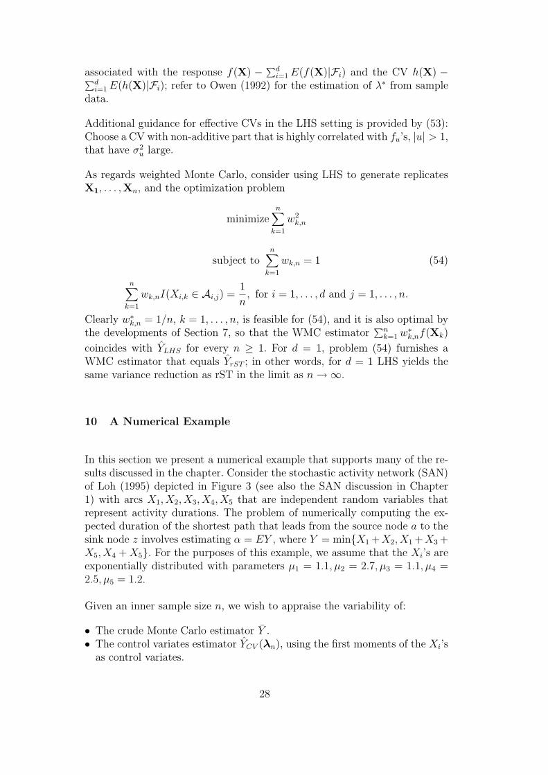
In this section we present a numerical example that supports many of the re-sults discussed in the chapter. Consider the stochastic activity network (SAN)of Loh (1995) depicted in Figure 3 (see also the SAN discussion in Chapter1) with arcs X1, X2, X3, X4, X5 that are independent random variables thatrepresent activity durations. The problem of numerically computing the ex-pected duration of the shortest path that leads from the source node a to thesink node z involves estimating α = EY , where Y = minX1 +X2, X1 +X3 +X5, X4 + X5. For the purposes of this example, we assume that the Xi’s areexponentially distributed with parameters µ1 = 1.1, µ2 = 2.7, µ3 = 1.1, µ4 =2.5, µ5 = 1.2.

Given an inner sample size n, we wish to appraise the variability of:

• The crude Monte Carlo estimator Y .• The control variates estimator YCV (λn), using the first moments of the Xi’s

as control variates.

28

• The conditional Monte Carlo estimator YCMC . Because the durations of thethree paths that lead from a to z are conditionally independent given X1

and X5, E(Y |X1, X5) can be found analytically; see Loh (1995, p. 103).• The weighted Monte Carlo estimator YWMC , with f(w) = − log w in Equa-

tion (38).• The stratification estimator YrST , where we stratify on X1.• The Latin hypercube estimator YLHS applied to X1, . . . , X5.

In order to compare the variance of these estimators, we repeat m = 1000times the simulation to obtain Y (m), . . . , YLHS(m) by averaging Y , . . . , YLHS

over m . The (sample) standard deviations of these six estimators are s(m, n),sCV (m,n), sCMC(m,n), sWMC(m,n), srST (m,n), and sLHS(m,n).

The results are summarized in Table 1. As expected, sCV (m,n) ≈ sWMC(m,n),and sLHS(m,n) < srST (m,n) for each n. Notice that srST (m,n) and sLHS(m,n)behave like a constant divided by n1/2 for each n, which indicates that rSTand LHS achieve their variance reduction potential by n = 100.

11 Conclusions

We presented various variance reduction techniques for terminating simula-tions in the Hilbert space setting, establishing connections with CV, CMC,and WMC whenever possible. It is the geometric interpretation of Result 2that makes this approach especially tractable.

There are, however, several topics missing from our coverage where Hilbertspace theory might yield valuable insights. Consider for instance the case ofvariance reduction techniques for steady-state simulations that have a suitablemartingale representation; see, for example, Henderson and Glynn (2002). It is

"!

#Ã

"!

#Ã"!

#Ã

"!

#Ã

´´

´´

´´3

´´

´´

´´3

QQ

QQ

QQQs

QQ

QQ

QQQs

?

a z

X1 X2

X4 X5

X3

Fig. 3. Stochastic Activity Network

29

Sample size n

Parameter 100 1000 10000

s(m,n) 0.0529 0.0162 0.0053

sCV (m, n) 0.0392 0.0112 0.0036

sCMC(m,n) 0.0328 0.0102 0.0033

sWMC(m,n) 0.0395 0.0116 0.0038

srST (m,n) 0.0456 0.0144 0.0044

sLHS(m,n) 0.03 0.0093 0.0030

Table 1. SAN Numerical Example

well-known that square integrable martingale differences have a simple inter-pretation in the Hilbert space framework, which suggests that it might be pos-sible to obtain additional insights when dealing with such techniques. Anotherarea of interest is the Hilbert space formulation of CVs in the multi-responsesetting, where Y is a random vector; see Rubinstein and Marcus (1985) forrelevant results. The combination of importance sampling (cf. Chapter 12)with CVs also can be studied in the Hilbert space setting; see, for example,Hesterberg (1995), and Owen and Zhou (1999).

Acknowledgements

I would like to thank the editors for their valuable comments and suggestions.This work was supported by NPS grant RIP BORY4.

References

Avellaneda, M., Buff, R., Friedman, C., Grandchamp, N., Kruk, L., Newman,J., 2001. Weighted Monte Carlo: A new technique for calibrating asset-pricing models. International Journal of Theoretical and Applied Finance4, 1–29.

Avellaneda, M., Gamba, R., 2000. Conquering the Greeks in Monte Carlo:efficient calculation of the market sensitivities and hedge-ratios of financialassets by direct numerical simulation. Quantitative Analysis in FinancialMarkets, Vol. III. World Scientific, Singapore, pp. 336–356, M. Avellaneda(ed.).

Avramidis, A. N., Wilson, J. R., 1996. Integrated variance reduction tech-niques for simulation. Operations Research 44, 327–346.

30

Billingsley, P., 1995. Probability and Measure, 3rd Edition. John Wiley, NewYork.

Bollobas, B., 1990. Linear Analysis. Cambridge University Press, Cambridge.Durrett, R., 1996. Probability: Theory and Examples, 2nd Edition. Duxbury

Press, Belmont.Fishman, G. S., 1996. Monte Carlo: Concepts, Algorithms, and Applications.

Springer-Verlag, New York.Glasserman, P., 2004. Monte Carlo Methods in Financial Engineering.

Springer-Verlag, New York.Glasserman, P., Heidelberger, P., Shahabuddin, P., 1999. Asymptotically op-

timal importance sampling and stratification for path-dependent options.Mathematical Finance 9, 117–152.

Glasserman, P., Yu, B., 2005. Large sample properties of weighted MonteCarlo. Operations Research 53 (2), 298–312.

Glynn, P. W., Szechtman, R., 2002. Some new perspectives on the methodof control variates. Monte Carlo and Quasi-Monte Carlo Methods 2000.Springer-Verlag, Berlin, pp. 27–49, K. T. Fang, F. J. Hickernell, and H.Niederreiter (ed.).

Glynn, P. W., Whitt, W., 1989. Indirect estimation via L = λW . OperationsResearch 37, 82–103.

Henderson, S., Glynn, P. W., 2002. Approximating martingales for variance re-duction in Markov process simulation. Mathematics of Operations Research27, 253–271.

Hesterberg, T. C., 1995. Weighted average importance sampling and defensivemixture distributions. Technometrics 37 (2), 185–194.

Hesterberg, T. C., Nelson, B. L., 1998. Control variates for probability andquantile estimation. Management Science 44, 1295–1312.

Jiang, T., 2003. Data driven shrinkage strategies for quasi-regression. Ph.D.thesis, Stanford University.

Kreyszig, E., 1978. Introductory Functional Analysis with Applications. JohnWiley, New York.

Lavenberg, S. S., Moeller, T. L., Welch, P. D., 1982. Statistical results on con-trol variates with application to queueing network simulation. OperationsResearch 30, 182–202.

Lavenberg, S. S., Welch, P. D., 1981. A perspective on the use of controlvariables to increase the efficiency of Monte Carlo simulations. ManagementScience 27, 322–335.

Law, A. M., Kelton, W. D., 2000. Simulation Modeling and Analysis, 3rdEdition. McGraw-Hill, New York.

Loh, W. L., 1996. On Latin hypercube sampling. The Annals of Statistics24 (5), 2058–2080.

Loh, W. W., 1995. On the method of control variates. Ph.D. thesis, StanfordUniversity.

Mathe, P., 2000. Hilbert space analysis of Latin hypercube sampling. Proceed-ings of the American Mathematical Society 129 (5), 1477–1492.

31

McKay, M. D., Conover, W. J., Beckman, R. J., 1979. A comparison of threemethods for selecting values of input variables in the analysis of output froma computer code. Technometrics 21 (2), 239–245.

Nelson, B. L., 1990. Control variate remedies. Operations Research 38, 974–992.

Owen, A. B., 1992. A central limit theorem for Latin hypercube sampling.Journal of the Royal Statistical Society B 54 (2), 541–551.

Owen, A. B., 1997. Monte Carlo variance of scrambled equidistributionquadrature. SIAM Journal of Numerical Analysis 34 (5), 1884–1910.

Owen, A. B., Zhou, Y., 1999. Safe and effective importance sampling. Tech.rep., Stanford University.

Rubinstein, R. Y., Marcus, R., 1985. Efficiency of multivariate control variatesin Monte Carlo simulation. Operations Research 33, 661–677.

Schmeiser, B. W., Taaffe, M. R., Wang, J., 2001. Biased control-variate esti-mation. IIE Transactions 33, 219–228.

Serfling, R. J., 1980. Approximation Theorems of Mathematical Statistics.John Wiley, New York.

Stein, M., 1987. Large sample properties of simulations using Latin hypercubesampling. Technometrics 29, 143–151.

Szechtman, R., Glynn, P. W., 2001. Constrained Monte Carlo and the methodof control variates. In: Proceedings of the 2001 Winter Simulation Confer-ence. Institute of Electrical and Electronic Engineers, Piscataway, NJ, pp.394–400, B. A. Peters, J. S. Smith, D. J. Medeiros, and M. W. Rohrer (ed.).

Venkatraman, S., Wilson, J. R., 1986. The efficiency of control variates inmultiresponse simulation. Operations Research Letters 5, 37–42.

Williams, D., 1991. Probability with Martingales. Cambridge University Press,Cambridge.

Wilson, J. R., 1984. Variance reduction techniques for digital simulation.American Journal of Mathematical and Management Sciences 4, 277–312.

Zimmer, R. J., 1990. Essential Results of Functional Analysis. The Universityof Chicago Press, Chicago.

32