chapter 1 the theory of turing pattern formation · february 16, 2004 11:1 wspc/trim size: 9.75in x...

February 16, 2004 11:1 WSPC/Trim Size: 9.75in x 6.5in for Review Volume review

CHAPTER 1

The theory of Turing pattern formation

Teemu Leppanen

Helsinki University of Technology, Laboratory of Computational EngineeringP.O.Box 9203, FIN-02015 HUT, FINLAND E-mail: [email protected]

In this article the theory behind Turing instability in reaction-diffusion systemsis reviewed. The use of linear analysis and nonlinear bifurcation analysis withcenter manifold reduction for studying the behavior of Turing systems is pre-sented somewhat meticulously at an introductory level. The symmetries that areconsidered here in the context of a generic Turing model are the two-dimensionalhexagonal lattice and three-dimensional SC- and BCC-lattices.

1. Introduction

The self-organization of dissipative structures is a phenomenon typical to non-

equilibrium systems. These structures exist far from equilibrium and differ from

typical equilibrium structures (eg. crystals) in that they are kept in the steady-state

by competing ongoing dynamic processes, which feed energy into the system. The

structures persist by dissipating the input energy (and thus generating entropy),

which makes the process irreversible. Dissipative structures are typically macro-

scopic and the characteristic length scale of the structure is independent of the size

of the individual constituents (eg. molecules) of the system. The systems repre-

senting self-organized dissipative structures vary from growing bacterial colonies to

fluids with convective instabilities (eg. Rayleigh-Benard convection).1,2

The formal theory of self-organization is based on non-equilibrium

thermodynamics3 and was pioneered by chemist Ilya Prigogine. Most of the re-

search was made in Brussels from the 1940s to 1960s by Prigogine and coworkers.

They extended the treatment of non-equilibrium thermodynamic systems to non-

linear regime far from equilibrium and applied bifurcation theory to analyze the

state selection.4 Already in 1945 Prigogine had suggested that a system in non-

equilibrium tries to minimize the rate of entropy production and chooses the state

accordingly.5 This condition was proved inadequate by Rolf Landauer in 1975, who

argued that minimum entropy production is not in general a necessary condition

for the steady-state and that one cannot determine the most favorable state of the

system based on the behavior in the vicinity of the steady state, but one must

consider the global non-equilibrium dynamics.6 Nevertheless, in 1977 Prigogine was

1


2 T. Leppanen

awarded the Nobel price in chemistry for his contribution to the theory of dissipative

structures.

This article does not deal with the so far incomplete theory of non-equilibrium

thermodynamics, but with chemical systems, which can exhibit instabilities result-

ing in either oscillatory or stationary patterns.7,8 The difficulties of non-equilibrium

thermodynamics are also present in the theory of chemical pattern formation. We

will specifically concentrate in systems showing so called Turing instability, which

arises due to different diffusion rates of reacting chemical substances. Turing in-

stability can be thought as a competition between activation by a slow diffusing

chemical (activator) and inhibition by a faster chemical (inhibitor). The idea of

diffusion-driven instability was first discussed by Nicolas Rashevsky in 19389, but

the renown British mathematician and computer scientist Alan Turing has earned

most of the fame for giving the first mathematical treatment and analysis of such

a model in 1952.10

Turing’s motivation for studying the chemical system was biological and conse-

quently the seminal paper was titled The Chemical Basis of Morphogenesis, where

he called the reacting and diffusing chemicals morphogens. Turing emphasized that

his model is very theoretical and a severe simplification of any real biological system,

but he was still confident that his model could explain some of the features related

to the spontaneous symmetry-breaking and morphogenesis, i.e., the growth of form

in nature. Turing neglected the mechanical and electrical aspects and considered the

diffusion and reaction of morphogens in the tissue to be more important.10 Nowa-

days, there is some qualitative evidence of the capability of Turing models to imitate

biological self-organization11,12,13, but the conclusive proof that morphogenesis is

indeed a Turing-like process is still missing.

The problem of Turing’s theory was that the existence of chemical spatial pat-

terns as predicted by his mathematical formulations could not be confirmed ex-

perimentally. The existence of Turing patterns in any chemical system could be

questioned not to talk about the biological systems. Actually, in the early 1950s

a Russian biochemist Boris Belousov observed an oscillation in a chemical reac-

tion, but he could not get his results published in any journal, because he could

not explain the results, which were claimed to contradict with the second law of

thermodynamics. Prior to Prigogine’s work it was held that entropy has to always

increase in a process and thus a chemical oscillation was deemed to be impossible

with entropy increasing and decreasing by turns. It was not before the late 1960s,

when it was noticed that the reaction first observed by Belousov exhibits a pat-

tern formation mechanism with similarities to the mechanism Turing had proposed.

However, it is important to notice that the Belousov-Zhabotinsky reaction forms

traveling waves, whereas Turing patterns are time-independent.

The first experimental observation of stationary Turing patterns was preceded by

theoretical studies14,15 and the practical development of a new kind of continuously

stirred tank reactors.16 It was not until 1990, when Patrick De Kepper’s group


The theory of Turing pattern formation 3

observed a stationary spotty pattern in a chemical system involving the reactions

of chlorite ions, iodide ions and malonic acid (CIMA reaction).17 In particular the

required difference in the diffusion rates of the chemical substances delayed the first

experimental observation of Turing patterns. In the experiment the condition was

achieved by carrying out the experiment in a slab of polymer gel and using a starch

indicator, which decreases the diffusion rate of the activator species (iodide ions).

In 1991 also stripes were observed in the CIMA reaction and it was shown that

experimental Turing patterns can be grown also over large domains.18

The observation of Turing patterns initiated a renewed interest in Turing pattern

formation. What had previously been only a mathematical prediction of an inge-

nious mathematician was 40 years later confirmed to be a real chemical phenomenon.

This article introduces the reader to the theoretical background and mathematical

formalism related to the study of Turing pattern formation. I will introduce the

reader to the idea of Turing instability and to the mathematical models that gen-

erate Turing patterns in Sec. 2. In Sec. 3 the same topics will be discussed from a

more mathematical point of view. In Sec. 4 the methods of the bifurcation theory

will be applied to the study of the pattern (2D) or structure (3D) selection in a

generic Turing model.

2. Turing instability

The traveling wave patterns generated by the Belousov-Zhabotinsky reaction are

not due to Turing instability since the diffusion rates of the chemicals involved

in that reaction are usually more or less the same. The difference in the diffusion

rates of the chemical substances is a necessary, but not a sufficient condition for

the diffusion-driven or Turing instability. Turing’s idea that diffusion could make a

stable chemical state unstable was innovative since usually diffusion has a stabilizing

effect (e.g. a droplet of ink dispersing into water). Intuitively Turing instability can

be understood by considering the long-range effects of the chemicals, which are not

equal due to difference in the pace of diffusion and thus an instability arises. Some

exhilarating common sense explanations of the mechanism of the instability can be

found from the literature: Murray has discussed sweating grasshoppers on a dry

grass field set alight11 and Leppanen et al. have tried to illustrate the mechanism

by using a metaphor of biking missionaries and hungry cannibals on an island.19

Turing begun his reasoning by considering the problem of a spherically symmet-

rical fertilized egg becoming a complex and highly structured organism. His purpose

was to propose a mechanism by which the genes could determine the anatomical

structure of the developing organism. He assumed that genes (or proteins and en-

zymes) act only as catalysts for spontaneous chemical reactions, which regulate

the production of other catalysts or morphogens. There was not any new physics

involved in Turing’s theory. He merely suggested that the fundamental physical

laws can account for complex physico-chemical processes. If one has a spherically

symmetrical egg, it will remain spherically symmetrical forever notwithstanding the


4 T. Leppanen

chemical diffusion and reactions. Something must make the stable spherical state

unstable and thus cause spontaneous symmetry-breaking. Turing hypotetized that

a chemical state, which is stable against perturbations, i.e., returns to the stable

state in the absence of diffusion may become unstable against perturbations in the

presence of diffusion. The diffusion-driven instability initiated by arbitrary random

deviations results in spatial variations in the chemical concentration, i.e., chemical

patterns.10

No egg in the blastula stage is exactly spherically symmetrical and the random

deviations from the spherical symmetry are different in two eggs of the same species.

Thus one could argue that those deviations are not of importance since all the or-

ganisms of a certain species will have the same anatomical structure irrespective

of the initial random deviations. However, Turing emphazised and showed that “it

is important that there are some deviations for the system may reach a state of

instability in which these irregularities tend to grow”.10 In other words, if there are

no random deviations, the egg will stay in the spherical state forever. In biological

systems the random deviations arise spontaneously due to natural noise and distor-

tions. A further unique characteristic of the Turing instability is that the resulting

chemical pattern (or biological structure) is not dependent on the direction of the

random deviations, which are necessary for the pattern to arise. The morphological

characteristics of the pattern, e.g. whether it is stripes or spots, are determined by

the rates of the chemical reactions and diffusion. That is, the morphology selection

is regulated intrinsically and not by external length scales (as in the case of many

convective instabilities2).

The random initial conditions naturally have an effect on the resulting pattern,

but only with respect to the phase of the pattern. The intrinsic parameters de-

termine that the system will evolve to stripes of a fixed width, but the random

initial conditions determine the exact positions and the alignment of the stripes

(the phase). The relevance of Turing instability is not confined to chemical sys-

tems, but also many other physical systems exhibiting dissipative structures can

be understood in terms of diffusion-driven instability. Turing instability has been

connected to gas discharge systems20, catalytic surface reactions21, semiconductor

nanostructures22, nonlinear optics23, irradiated materials24 and surface waves on

liquids25. In this article I will concentrate solely on reaction-diffusion Turing sys-

tems.

3. Linear theory

In this section the mathematical formulation of Turing models is introduced, the

Turing instability is discussed using mathematical terms and analyzed by employing

linear stability analysis. We will witness the strength of linear analysis in predict-

ing the instability and the insufficiency of it in explaining pattern selection. The

nonlinear analysis required for explaining pattern selection will be presented in the

next section.



Let us denote two space- and time-dependent chemical concentrations by U(~x, t)

and V (~x, t), where ~x ∈ Ω ⊂ n denotes the position in an n-dimensional space,

t ∈ [0,∞) denotes time and Ω is a simply connected bounded domain. Using

these notations one can derive a system of reaction-diffusion equations from first

principles11 and they are given as follows

Ut = DU∇2U + f(U, V )

Vt = DV ∇2V + g(U, V ), (1)

where U ≡ U(~x, t) and V ≡ V (~x, t) are the morphogen concentrations, and DU

and DV the corresponding diffusion coefficients setting the time scales for diffusion.

The diffusion coefficients must be unequal for the Turing instability to occur in two

or more dimensions26. One should notice that Eq. (1) is actually a system of two

diffusion equations, which are coupled via the kinetic terms f and g describing the

chemical reactions. This reaction-diffusion scheme is generalizable to any number

of chemical species, i.e., equations.

The form of the reaction kinetics f and g in Eq. (1) determines the behavior

of the system. These terms can be derived from the chemical formulae describing

the reaction by using the law of mass action11 or devised based phenomenological

considerations. There are numerous possibilities for the exact form of the reaction

kinetics including the Gray-Scott model27,28,29,30, the Gierer-Meinhardt model31,

the Selkov model32,33, the Schnackenberg model34,35, the Brysselator model4,36 and

the Lengyel-Epstein model14,37,38. These all models consist of two coupled reaction-

diffusion equations and exhibit the Turing instability within a certain parameter

range. The Lengyel-Epstein model is the only one, which corresponds to a real

chemical reaction (the experimentally observed CIMA reaction). The presence of

some nonlinear term in f and g is common to all these models. A nonlinearity is

required since it bounds the growth of the exponentially growing unstable modes.

The stationary state (Uc, Vc) of a model is defined by the zeros of the reaction

kinetics, i.e., f(Uc, Vc) = g(Uc, Vc) = 0. Typically the models are devised in such

a manner that they have only one stationary state, but some models have more.

With certain parameters the stationary state is stable against perturbations in the

absence of diffusion, but in the presence of diffusion the state becomes unstable

against perturbations. If we initialize the system to the stationary state, it will

remain there forever. If we perturb the system around the stationary state in the

absence of diffusion, the system will return to its original state, i.e., the state is

stable. However, when we perturb the system in the presence of diffusion arbitrarily

around the stationary state, the perturbations will grow due to the diffusion-driven

instability, i.e., the state is unstable. Mathematical definitions of stability can be

found from the literature.40

All the analysis in this article will be carried out using a generic Turing model

introduced by Barrio et al.39 This model is a phenomenological model, where the

reaction kinetics are obtained by Taylor expanding the nonlinear functions around


6 T. Leppanen

a stationary solution (Uc, Vc). If terms of the fourth and higher order are neglected,

the reaction-diffusion equations can be written as

ut = Dδ∇2u + αu(1 − r1v2) + v(1 − r2u)

vt = δ∇2v + v(β + αr1uv) + u(γ + r2v), (2)

where the concentrations have been normalized so that u = U −Uc and v = V −Vc,

which makes (uc, vc) = (0, 0) a stationary state. The parameters r1, r2, α, β and γ

have numerical values and they define the reaction kinetics. The diffusion coefficients

are written in terms of a scaling factor δ and the ratio D. We must always have

D 6= 1 for the instability.

To reduce the number of parameters and simplify the analysis we carry out non-

dimensionalization11 of the Eq. (2) by rescaling the parameters, concentrations and

the time and length scales. This yields the system

ut = D∇2u + ν(u + av − uv2 − Cuv)

vt = ∇2v + ν(bv + hu + uv2 + Cuv), (3)

where the concentrations are scaled such that (u, v) = 1√r1

(u, v) and the time-space

relation is given by T = L2/δ (t = Tτ and x = Lx). In the terms of the original

parameters, the new parameters are C = r2/(α√

r1), a = 1/α, b = β/α, h = γ/α

and ν = αT . The term C adjusts the relative strength of the quadratic and cubic

nonlinearities favoring either stripe or spot selection.39 From now on we omit the

overlines for simplicity.

One can easily see that the system of Eq. (3) has a stationary state at (uc, vc) =

(0, 0). For h 6= −1 the system has also two other stationary states defined by

f(uc, vc) = g(uc, vc) = 0 and they are given by

uic = −vi

c/K, (4)

and

vic =

−C + (−1)i ±√

C2 − 4(h − bK)

2(5)

where K = 1+ha+b and i = 1, 2.

Linear analysis is a generally used method for evaluating the behavior of per-

turbations in a nonlinear system in the vicinity of a stationary state.11,40,41 In the

linear analysis one takes into account only the linear terms and thus the results are

insufficient. However, within its limitations the method is typically quite efficient

in predicting the existence of an instability and the characteristic wave length of

it. The linearized system in the absence of diffusion can be written in the form

~wt = A~w and reads as(

ut

vt

)

=

(

fu fv

gu gv

)

uc,vc

(

u

v

)

, (6)



where fu, fv, gu and gv in the matrix A denote the partial derivatives of the reaction

kinetics evaluated at the stationary state (uc, vc). In the case of Eq. (3) the linearized

matrix is given as

A = ν

(

1 − v2c − Cvc −2ucvc + a − Cuc

v2c + h + Cvc b + 2ucvc + Cuc

)

, (7)

where uc and vc are given by Eqs. (4) and (5). In the linear analysis the spatial

and time variance are taken into account by substituting a trial solution of the form

w(~r, t) =∑

k ckeλtwk(~r, t) into the linearized system in the presence of diffusion.

The eigenvalues of this linearized system are obtained from the equation

|A −Dk2 − λI| = 0, (8)

where A is given by Eq. (6), D11 = Du, D22 = Dv, D12 = D21 = 0 and I is the

identity matrix in the general case. In the case of Eq. (3) A is given by Eq. (7), and

D11 = D and D22 = 1. The determinant in Eq. (8) can be solved, which yields the

equation

λ2 +[

(Du + Dv)k2 − fu − gv

]

λ + DuDvk4 − k2(Dvfu + Dugv) + fugv − fvgu = 0,(9)

where k2 = ~k ·~k. The dispersion relation λ(k) predicting the unstable wave numbers

can be solved from Eq. (9). One can obtain an estimate for the most unstable wave

number and the critical value of the bifurcation parameter by considering the fact

that at the onset of the instability λ(kc) = 0. Thus the term independent of λ in

Eq. (9) must be zero at kc. In the case of the generic Turing model this condition

reads as

Dk4c − k2

cν(Db + 1) + ν2(b − ah) = 0. (10)

At the onset this equation has only one solution given by k2c = ν(Db + 1)/(2D),

which takes place for the bifurcation parameter value a = ac = −(Db− 1)2/(4Dh).

An instability exists for a < ac. The conditions for the Turing instability are widely

known8,11 to be the following

fu + gv < 0

fugv − fvgu > 0

Dvfu + Dugv > 0. (11)

Based on linear analysis and numerical observations it can be deduced that for

h < −1 stationary state (0, 0) is no more unstable and one of the other stationary

states shows a Hopf-like bifurcation to a damped time-dependent oscillatory state

without a characteristic length scale. On the other hand, for h > −1 there is a

coupling of Turing instability with a characteristic length (bifurcation of the state

(0,0)) and a time-dependent instability with k = 0 unstable (bifurcation of the

state defined by Eq. (5) with i = 1), which results in a transient large amplitude

competition between oscillatory and fixed length scale instability. To simplify the


8 T. Leppanen

study of the generic model of Eq. (3), we will fix h = −1 from now on. This makes

the (0, 0) the only stationary state and simplifies our analysis.

In the case of the generic model with h = −1 the above conditions (Eq. (11))

and the previous reasoning yield the constraints −b < a < ac = (Db−1)2/(4D) and

−1/D < b < −1 for the Turing instability. Based on this one can sketch the stability

diagram for the generic Turing model. This is presented in Fig. 1. From the stability

diagram one can notice that the number of the parameter sets exhibiting Turing

instability, i.e., the size of the Turing space (shaded region) is relatively small. For

explanations of the other regions of the diagram see the caption.

-2 -1.5 -1 -0.5 0b

0

0.5

1

1.5

2

a

33

4 4

2

2

Fig. 1. The stability diagram of the generic Turing model (Eq. (3)). The Turing space (shadedregion) is bounded by lines b = −1/D, b = −1, b = −a and the curve a = (Db− 1)2/(4D). For theplot parameters were fixed to D = 0.516. The other regions: stable state (2), other instabilities (3)and Hopf instability (4).

Based on the stability diagram one can choose parameters that result in the

Turing instability. Here we use two sets of parameters that have been used earlier

in the case of the generic Turing model.39,42 For the non-dimensionalized generic

model (with L = 1) the parameters are given as D = 0.516, a = 1.112, b = −1.01



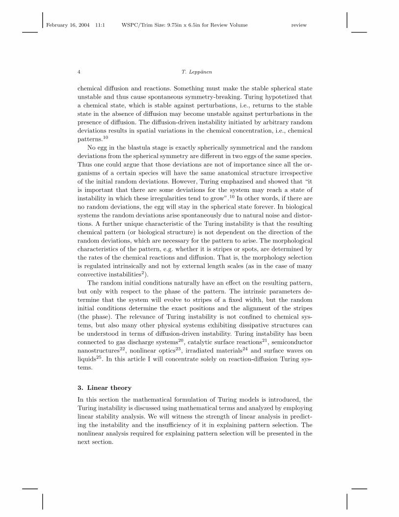
and ν = 0.450 for kc = 0.46 (ac = 1.121) and D = 0.122, a = 2.513, b = −1.005 and

ν = 0.199 for kc = 0.85 (ac = 2.583). The dispersion relation is obtained by solving

Eq. (9) with respect to λ and plotting the real part of the solution. The dispersion

relations corresponding to the onset of the instability (at a = ac) and the above

parameter sets resulting in the instability are shown in Fig. 2. The growing modes

are of the form Aei~k·~reλ(k). Thus the wave numbers k with Reλ(k) < 0 will be

damped, whereas the wave numbers with Reλ(k) > 0 will grow exponentially

until the nonlinearities bound the growth. The dispersion relations in Fig. 2 tells us

the growing modes and predicts the characteristic length of the pattern. The wave

number and the wave length are related by λ = 2π/k.

0 0.1 0.2 0.3 0.4 0.5 0.6 0.7 0.8 0.9 1k

-0.2

-0.15

-0.1

-0.05

0

Re

λ(k)

0 0.1 0.2 0.3 0.4 0.5 0.6 0.7 0.8 0.9 1k

-0.2

-0.15

-0.1

-0.05

0R

eλ(

k)

Fig. 2. The dispersion relations λ(k) corresponding to two different parameter sets with kc = 0.46and kc = 0.85, respectively. Left: At the onset of instability a = ac and there are no unstable modes.Right: For a < ac there is a finite wave length instability corresponding to wave numbers k forwhich Reλ(k) > 0.

Due to the width of the unstable wave window (Fig. 2), there is more than one

unstable mode. The unstable modes that do not correspond to kc, i.e., the highest

point of the dispersion relation are called the sideband. The side band widens with

the distance to onset ac − a as the bifurcation parameter a is varied. The linear

analysis does not tell, which of these unstable modes will be chosen. In addition,

there is degeneracy due to isotropy, i.e., there are many wave vector ~k having the

same wave number k = |~k|. In a discrete three-dimensional system the wave number

is given by

|~k| = 2π

√

(

nx

Lx

)2

+

(

ny

Ly

)2

+

(

nz

Lz

)2

, (12)

where Lx/y/z denote the system size in respective directions and nx/y/z the re-

spective wave number indices. For a one-dimensional system ny = nz = 0 and for

a two-dimensional system nz = 0. Based on Eq. (12) one notices that e.g. two-

dimensional vectors (kc, 0), (0, kc) and (kc/√

2, kc/√

2) all correspond to the wave


10 T. Leppanen

number kc and thus they are all simultaneously unstable. Actually, in a continuous

system there would be an infinite number of unstable wave vectors pointing from

the origin to the perimeter of a circle with a radius kc. To tackle the problem of

pattern selection, i.e., which of the degenarate modes will contribute to the final

pattern a nonlinear analysis is required.

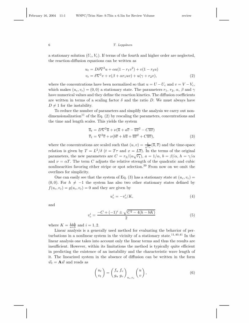
Fig. 3. Chemical concentration patterns obtained from numerical simulations of the Eq. (3) in asystem sized 128 × 128. Left: Stripe pattern (kc = 0.85, C = 0). Right: Hexagonal spotty pattern(kc = 0.46, C = 1.57). See the text for the other parameters.

From the results of the linear analysis we can identify the parameter domain,

which results in the Turing instability and approximate the characteristic wave

length of the patterns. Fig. 3 shows a stripe pattern and a spotty pattern with

different characteristic lengths obtained from a numerical simulation with different

parameter values. These two morphologies are typical for reaction-diffusion systems

in two dimensions.43 The generic Turing model has been devised in such a way that

by adjusting parameter C one can favor either stripe or spotty patterns.39,42 The

rigorous proof of this requires nonlinear bifurcation analysis and is the subject of

the next section.

4. Nonlinear bifurcation theory

Bifurcation theory is a mathematical tool generally used for studying the dynamics

of nonlinear systems.44,45,46 The result of bifurcation analysis or weakly nonlinear

analysis is a qualitative approximation for the changes in the dynamics of the system

under study. In the case of Turing systems the bifurcation analysis answers the

question concerning the changes in the stability of different simple morphologies as

a parameter is varied. The bifurcation analysis has previously been applied in the

cases of the Brysselator model47 and the Lengyel-Epstein model48. The problem of

these published analyses is that they omit the mathematical details required for

understanding at an elementary level. In this section I will try to illustrate the idea



of bifurcation analysis and the related mathematical techniques in a meticulous

manner.

The idea of the bifurcation analysis is to find a presentation for the concentration

field ~w = (u, v)T in terms of the active Fourier modes, i.e.,

~w = ~w0

∑

~kj

(Wjei~kj ·~r + W ∗

j e−i~kj ·~r), (13)

where ~w0 defines the direction of the active modes. Wj and W ∗j are the amplitudes

of the corresponding modes ~kj and −~kj . Notice that the sum of complex conjugates

is real. The unstable modes have slow dynamics, whereas the stable modes relax

quickly and are said to be slaved to the unstable modes. Typically the bifurcation

analysis is carried out by observing changes as a function of the bifurcation param-

eter, i.e., the distance to onset. In the case of the generic Turing system (Eq. (3))

there is an additional quadratic nonlinearity, which is adjusted by parameter C.

This parameter governs the morphology selection between linear (stripe) and radial

(spot) structures instead of the bifurcation parameter and forces to some additional

algebraic manipulations at the end of the bifurcation analysis.

The bifurcation analysis can be divided into three parts: derivation of the nor-

mal form for the amplitude equations in a particular symmetry, determining the

parameters of the amplitude equations (there are various techniques for this) and

finally analyzing the stability of different morphologies by applying the linear anal-

ysis (Sec. 3) on the system of amplitude equations. These three phases will be the

respective topics of the following subsections.

4.1. Derivation of the amplitude equations

A system of n amplitude equations describes the time variation of the amplitudes Wj

of the unstable modes ~kj (j = 1, . . . , n). The amplitude equations contain a linear

part corresponding to the linear growth predicted by the positive eigenvalue of the

linearized system defined by Eq. (9) and a nonlinear part due to nonlinear coupling

of the unstable modes. Thus the most general form of an amplitude equation given

by

dWj

dt= λcWj + fj(W1, . . . , Wn). (14)

The eigenvalue may be approximated in the vicinity of the onset by a linear

approximation defined by

λc =dλ

da

∣

∣

∣

∣

a=ac

(a − ac) =ν2(ν − 2R)

(ν(1 + b) − 2R)(ν − R), (15)

where R = ν(Db + 1)/2 with notations of the generic Turing model (Eq. (3)).

The exact form of the term f(W1, . . . , Wn) in Eq. (14) depends on the symmetries

under study and may be constructed by geometrical arguments. In two dimensions

reaction-diffusion systems typically exhibit either stripes or a hexagonally arranged


12 T. Leppanen

spots (Fig. 3). Thus the natural selection for the study of 2D patterns is a hexagonal

lattice. In three dimensions there are various possibilities: One can study the simple

cubic lattice (SC), base-centered cubic lattice (BCC) or face-centered cubic lattice

(FCC).49 Callahan and Knobloch have been among the first to address the problem

of bifurcations in three-dimensional Turing systems.50,51,52 In the following we will

derive the amplitude equations for the two-dimensional hexagonal lattice and three-

dimensional SC- and BCC-lattices.

2D hexagonal lattice

The base vectors of a two-dimensional hexagonal lattice can be chosen to be ~k1 =

kc(1, 0), ~k2 = kc(−1/2,√

3/2) and ~k3 = kc(−1/2,−√

3/2) with |~k1,2,3| = kc. Since

−~k1 − ~k2 = ~k3 we can say that a hexagonal lattice exhibits resonant modes, which

one must take into account, while deriving the form of the amplitude equations. In

a simple square lattice there would not be any resonant modes, since any subset

of the base vectors does not sum into another base vector. The base vectors of a

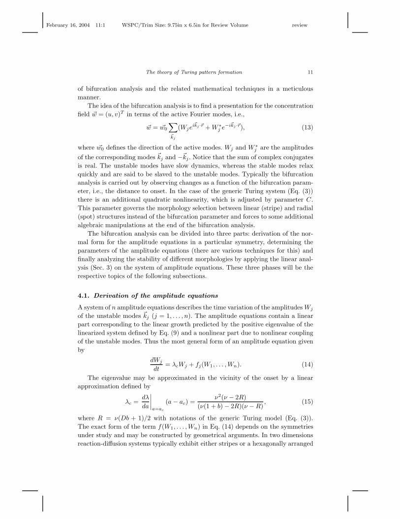
hexagonal lattice and the idea of resonant modes is illustrated in Fig. 4.

2k

3kk 1

k 1

2k2k k 12π/3 +=3k−

Fig. 4. The base vectors of a two-dimensional hexagonal lattice are not linearly independent andthus there are resonant modes.

Based on the above reasoning one would suggest that there must be a quadratic

coupling term in the amplitude equation: Since the negative sum of two other modes

may contribute to any one mode, there must be a term of the form (−W ∗j+1)(−W ∗

j+2)

in fj(W1, W2, W3) (j = 1, 2, 3 (mod 3)). The other combinations of wave vectors that

sum up to ~kj are ~kj −~kj +~kj , ~kj+1 −~kj+1 +~kj , and ~kj+2 −~kj+2 +~kj . The respective

contributions to fj(W1, W2, W3) are −|Wj |2Wj , −|Wj+1|2Wj and −|Wj+2|2Wj . We

assume that the saturation occurs at the third order and thus take into account

only the sums of maximum three vectors. Now the full amplitude equation for the



two-dimensional hexagonal lattice may be written as

dWj

dt= λcWj + ΓW ∗

j+1W∗j+2 − g[|Wj |2 + κ(|Wj+1|2 + |Wj+2|2)]Wj , (16)

where the coefficients Γ, g and κ can be presented in terms of the parameters of the

original reaction-diffusion system (Eq. (3)). The coefficients are obtained via com-

plicated mathematical techniques, which will be discussed in the next subsection.

3D SC-lattice

The base vectors of a three-dimensional simple cubic lattice can be chosen to be~k1 = kc(1, 0, 0), ~k2 = kc(0, 1, 0) and ~k3 = kc(0, 0, 1) with |~k1,2,3| = kc. Now the base

vectors are linearly independent and thus there are no resonant modes. By following

the same reasoning as in the case of 2D hexagonal lattice, one can deduce the form

of the amplitude equations to be the following

dWj

dt= λcWj − g[|Wj |2 + κ(|Wj+1|2 + |Wj+2|2)]Wj . (17)

3D BCC-lattice

The three-dimensional base-centered cubic lattice is a little bit more tricky. The set

of base vectors is ~k1 = kc(1, 1, 1)/√

3, ~k2 = kc(1, 1,−1)/√

3, ~k3 = kc(1,−1, 1)/√

3

and ~k4 = kc(1,−1,−1)/√

3 with |~k1,2,3,4| = kc. These are not linearly independent

since e.g. ~k2 + ~k3 − ~k4 = ~k1. Thus there is a cubic resonant coupling term and in

addition there are the other nonlinear terms. The amplitude equations are given by

dWj

dt= λcWj + ΓW ∗

j+1W∗j+2W

∗j+3 − g[|Wj |2 + κ(|Wj+1|2 + |Wj+2|2 + |Wj+3|2)]Wj ,

(18)

where (j = 1, 2, 3, 4 (mod 4)).

4.2. Center manifold reduction

There are various methods for determining the parameters for the amplitude equa-

tion. In the most used method, the multiscale expansion,44,47 the bifurcation pa-

rameter and the chemical concentrations are expanded in a small parameter (e.g.

a − ac = εa1 + ε2a2 + ...) and the coefficients are obtained based on the solvabil-

ity conditions of the resulting linear differential equations at different degrees of ε.

In this article we will not use multiscale expansion, but a related method called

the center manifold reduction45,52. We will take the method of center manifold re-

duction as given and for the mathematical justification of it we refer the reader

elsewhere.45,51,53

The purpose of the center manifold reduction is to devise a mapping from the

concentration space (Eq. (3)) to a high-dimensional equivariant amplitude space

(Eq. (14)). The center manifold is a surface separating the unstable and stable


14 T. Leppanen

manifolds in the wave vector space. The center manifold reduction confines the

nonlinear effects in the system to the center manifold and thus one can obtain good

approximations for the stability of different structures. In the following, we will

sketch the general procedure to obtain the amplitude equations following Callahan

and Knobloch52 to whom we refer the reader for details.

In general, we can write the component h of a Turing system with n chemical

species (h ∈ 1, ..., n) as

dXh

dt= Dh∇2W h+

n∑

i=1

Ah,iW i+

n∑

i=1

n∑

j=1

Ah,ijX iXj+

n∑

i=1

n∑

j=1

n∑

k=1

Ah,ijkX iXjXk+...

(19)

where Xh = Xh(~x, t) is the spatially varying concentration of one chemical species

and Xh = 0 in the uniform stationary state. The tensors Ah,i, Ah,ij and Ah,ijk

define the parameters for the component h and are symmetric with respect to

permutations of the indices. In a discrete system we can write the concentration in

a certain position of the lattice as

Xh(~x, t) =∑

l∈L

Xhl (t)ei~kl·l, (20)

where L is the set of all lattice points. From now on we write species indices

(e.g. h) as superscripts and lattice point indices (e.g. l) as subscripts. Substitut-

ing Eq. (20) into Eq. (19) yields

dXhl

dt= −Dh|~kl|2Xh

l + Ah,iX il + Ah,ij

∑

l1+l2=l

X il1X

jl2

+ Ah,ijk∑

l1+l2+l3=l

X il1X

jl2

Xkl3 ,

(21)

where we have used the Einstein summation convention for the indices i, j and k,

and included only the terms up to cubic order. The linear part the previous equation

defines the unstable modes (see Sec. 3) and the linear matrix can be written in the

form

Jh,il = −Dhk2

l δh,i + Ah,i, (22)

where it is assumed that there is no cross-diffusion (δh,i = 1 only when h = i). For

each lattice point we may now choose a matrix

Sl =

α11l . . . α1n

l...

. . ....

αn1l . . . αnn

l

, (23)

with det(Sl) = 1. In addition, we require that it has an inverse matrix S−1l = βij

l such that

S−1l JlSl =

λ1l

. . .

λnl

. (24)



The conditions for this similarity transformation are widely known.52,54 Now we can

map the original concentrations (Eq. (21)) to a new basis defined by S−1l Xl = Wl.

In this new basis Eq. (21) reads as

dW gl

dt= λg

l Wgl + βgh

l Ah,ij∑

l1+l2=l

αii′

l1 W i′

l1 αjj′

l2W j′

l2+

βghl Ah,ijk

∑

l1+l2+l3=l

αii′

l1 W i′

l1 αjj′

l2W j′

l2αkk′

l3 W k′

l3 . (25)

The coefficient of the linear term is defined by Eq. (15). The coefficients of the

nonlinear terms can be calculated at the onset by fixing a = ac and using the infor-

mation about stable and unstable modes. Using the fact that the only contribution

to the growth of the stable modes comes via a nonlinear coupling, one can derive

relations for the parameters.52 Further simplification of Eq. (25) for a critical wave

vector m at the onset (λgl = 0) yields

dW 1m

dt= β1hAh,ijαi1αj1

∑

m1+m2=m

W 1m1

W 1m2

+

∑

m1+m2+m3=m

F (m2 + m3)W1m1

W 1m2

W 1m3

, (26)

where

F (r) ≡ −2β1hAh,ijαi1(J−1r )jaAa,bcαb1αc1 + β1hAh,ijkαi1αj1αk1. (27)

One should notice that the coefficient F (r) depends on the argument r only through

the square of its length. Thus the previous treatment has been general and not

specific to any particular symmetry. In the following, we will derive the form of

the function F (r) for three different lattices in two or three dimensions. In order

to survive the horrendous linear algebra involved in the calculation, we follow a

computation procedure that has been used earlier.52 The derivation is based on

finding the number and type of resonant modes that contribute to the amplitude of

a particular mode as shown in Eq. (26). Due to symmetry, the coefficient of all the

amplitude equations in a particular amplitude system (Eq. (16) or (17) or (18)) are

the same.


In the hexagonal lattice two wave vectors sum up to another wave vector. The base

vectors for the hexagonal lattice are given by ~k1 = (1, 0), ~k2 = (−1/2,√

3/2) and~k3 = (−1/2,−

√3/2). The strength of the quadratic coupling term is determined

by the first term in Eq. (26). Since there are two possible selections (permutations)

of m1 and m2, i.e., −~k3 − ~k2 = −~k2 − ~k3 = ~k1 one has to take into account

both of them. Thus the quadratic coupling parameter in Eq. (16) is given by Γ =

2β1hAh,ijαi1αj1. The strength of the cubic coupling terms can be found by similar


16 T. Leppanen

arguments. However, there are two cases that have to be treated separately, case 1:

m1 = m2 6= m3 and case 2: m1 = m2 = m3.

In the first case the coupling is of the type k1 + k2 − k2 = k1. There are three

different combinations of m2 and m3 with two corresponding permutations. The

combinations are

(1) m2 = k2 and m3 = −k2 with |m2 + m3|2 = 0,

(2) m2 = k1 and m3 = k2 with |m2 + m3|2 = 1,

(3) m2 = k1 and m3 = −k2 with |m2 + m3|2 = 3,

which defines the coefficient gκ in Eq. (16) to have the value gκ = −2F (0)−2F (1)−2F (3).

In the second case the coupling is of the type k1 + k1 − k1 = k1. There are three

possible permutations with

(1) m2 = k1 and m3 = −k1 with |m2 + m3|2 = 0,

(2) m2 = −k1 and m3 = k1 with |m2 + m3|2 = 0,

(3) m2 = k1 and m3 = k1 with |m2 + m3|2 = 4,

which results in g = −2F (0)− F (4) for Eq. (16).

Based on the above reasoning and Eq. (27) one may calculate the exact form

of the coefficient in Eq. (16) with respect to the parameters of the generic Turing

model of Eq. (3). The parameters of the amplitude equations are given by

Γ =−2bCνR

√

ν(ν − 2R)

(ν + bν − 2R)√

(ν + bν − 2R)(ν − R), (28)

g =3bν2(ν − 2R)R

(ν + bν − 2R)2(ν − R), (29)

κ = 2, (30)

where we have denoted R = Dk2c = ν(Db + 1)/2. The linear coefficient of Eq. (16)

is given by Eq. (15).

3D SC-lattice

In the SC-lattice the base vectors are independent and given as ~k1 = (1, 0, 0),~k2 = (0, 1, 0) and ~k3 = (0, 0, 1). There are no resonant modes. Following the ideas

above in the first case we find

(1) m2 = k2 and m3 = −k2 with |m2 + m3|2 = 0,

(2) m2 = k1 and m3 = k2 with |m2 + m3|2 = 2,

(3) m2 = k1 and m3 = −k2 with |m2 + m3|2 = 2,

which defines the coefficient gκ = −2F (0) − 4F (2) in Eq. (16). The second case

yields the permutations

(1) m2 = k1 and m3 = −k1 with |m2 + m3|2 = 0,



(2) m2 = −k1 and m3 = k1 with |m2 + m3|2 = 0,

(3) m2 = k1 and m3 = k1 with |m2 + m3|2 = 4,

which gives g = −2F (0) − F (4) for Eq. (16).

For the amplitude equations of the three-dimensional SC-lattice (Eq. (17)) the

coefficients are given by

g =−bν2(C2(8ν − 23R) − 27R)(ν − 2R)

9(ν + bν − 2R)2(ν − R), (31)

κ =18(C2(8ν − 7R)− 3R)

C2(8ν − 23R) − 27R, (32)

where we have again denoted R = Dk2c = ν(Db + 1)/2 and the linear coefficient of

Eq. (17) is given by Eq. (15).

3D BCC-lattice

In the BCC-lattice the base vectors given by ~k1 = (1, 1, 1)/√

3, ~k2 = (1, 1,−1)/√

3,~k3 = (1,−1, 1)/

√3 and ~k4 = (1,−1,−1)/

√3 are not linearly independent. To find

the coefficient of the resonant contribution to Eq. (18) one must considers the pos-

sible combinations of the two last terms within the sum k2 + k3 − k4 = k1. These

are given by

(1) m2 = k3 and m3 = −k4 with |m2 + m3|2 = 43 ,

(2) m2 = −k4 and m3 = k2 with |m2 + m3|2 = 43 ,

(3) m2 = k2 and m3 = k3 with |m2 + m3|2 = 43 ,

which yields the resonant coupling coefficient Γ = 6F ( 43 ) for the Eq. (18).

The two other coefficient are determined using the same reasoning as above. In

the first case one gets

(1) m2 = k2 and m3 = −k2 with |m2 + m3|2 = 0,

(2) m2 = k1 and m3 = −k2 with |m2 + m3|2 = 43 ,

(3) m2 = k1 and m3 = k2 with |m2 + m3|2 = 83 ,

which results in the coefficient gκ = −2F (0) − 2F ( 43 ) − 2F ( 8

3 ) for the Eq. (18). In

the second case we get the permutations

(1) m2 = k1 and m3 = −k1 with |m2 + m3|2 = 0,

(2) m2 = −k1 and m3 = k1 with |m2 + m3|2 = 0,

(3) m2 = k1 and m3 = k1 with |m2 + m3|2 = 4,

which yields g = −2F (0) − F (4) for the Eq. (18).


18 T. Leppanen

The coefficients of the amplitude equations of the three-dimensional BCC-lattice

(Eq. (18)) can be written as

Γ =6bν2(ν − 2R)(3C2(8ν − 7R) − R)

(ν + bν − 2R)2(ν − R), (33)

g =−bν2(C2(8ν − 23R) − 27R)(ν − 2R)

9(ν + bν − 2R)2(ν − R), (34)

κ =18(C2(648ν − 583R)− 75R)

25(C2(8ν − 23R)− 27R), (35)

where R = ν(Db+1)/2 and the linear coefficient λc of Eq. (18) is defined by Eq. (15).

4.3. Stability of different structures

After we have obtained the system of coupled amplitude equations written with

respect to the parameters of the original reaction-diffusion equations, we may now

employ linear analysis to study the amplitudes. First one has to determine the

stationary states Wc of the amplitude system, which depends on the symmetry

under study (Eq. (16), (17) or (18)). After that one can linearize the system (as

in Eq. (6)) and construct the corresponding Jacobian linear matrix A, which is

determined by

Aij =

∣

∣

∣

∣

dfi

d|Wj |

∣

∣

∣

∣

(W c1

,W c2

,W c3)

, (36)

where fi denotes the right-hand side of the corresponding amplitude equation i and

the element is evaluated at the stationary state Wc = (W c1 , W c

2 , W c3 ). Based on this

one can plot the bifurcation diagram, i.e., the eigenvalues of the linearized system

dW/dt = AW as a function of the parameter C in Eq. (3), which contributes to the

morphology selection in the generic Turing model. The parameters of the generic

Turing model that we have used in the analysis presented here correspond to the

mode kc = 0.85 (see Fig. 2).


In the case of two-dimensional patterns we are interested in the stability of stripes

(Wc = (W c1 , 0, 0)T ) and hexagonally arranged spots (Wc = (W c

1 , W c2 , W c

3 )T with

W c1 = W c

2 = W c3 ). For the stability analysis of rhombic patterns and anisotropic

mixed amplitude states we refer the reader elsewhere.55 The system of amplitude

equations for a two-dimensional hexagonal lattice can be written based on Eq. (16)

asdW1

dt= λcW1 + ΓW ∗

2 W ∗3 − g[|W1|2 + κ(|W2|2 + |W3|2)]W1,

dW2

dt= λcW2 + ΓW ∗

1 W ∗3 − g[|W2|2 + κ(|W1|2 + |W3|2)]W2,

dW3

dt= λcW3 + ΓW ∗

1 W ∗2 − g[|W3|2 + κ(|W1|2 + |W2|2)]W3, (37)



where the coefficients λc, Γ, g and κ are given by Eqs. (15), (28), (29) and (30),

respectively. In the case of stripes W c2 = W c

3 = 0 and the system reduces to only one

equation. Now the stationary states defined by the zeros of the right-hand side of

Eqs. (37) can easily be shown to be W c1 =

√

λc

g eiφ1 . In the case of hexagonal spots

we have three equations and by choosing a solution such that Wc = W c1 = W c

2 = W c3

we obtain the two stationary states defined by

|W c±| =

|Γ| ±√

Γ2 + 4λcg[1 + 2κ]

2g(1 + 2κ). (38)

In the case of stripes the eigenvalues of the linearized matrix (Eq. (36)) are given

as µs1 = −2λc, µs

2 = −Γ√

λc

g +λc(1−κ) and µs3 = Γ

√

λc

g +λc(1−κ). Noticing that

µs1 < 0 and µs

3 > µ2 follows that the stability of stripes is determined by the sign

of µs3. The stripes are unstable for µs

3 > 0 and stable for µs3 < 0.

In the case of the hexagonally arranged spots the eigenvalues of the system are

given as µh1,2 = λc−W±

c (Γ+3gW±c ) and µh

3 = λc +W±c (2Γ−3g(2κ+1)W±

c ), where

W±c is defined by Eq. (38). Since there are two stationary states corresponding to

hexagonal symmetry one must analyze the stability of both of them. For stability

all the eigenvalues must be negative, i.e., µh1,2 < 0 and µh

3 < 0. After writing the

eigenvalues in terms of the original parameters (Eqs. (15), (28), (29), (30)) one can

plot the eigenvalues as a function of the nonlinear coefficient C, which is known to

adjust the competition between stripes and spots.39 The result is shown in Fig. 5,

from where one can determine the parameter regimes for which a given pattern is

stable, i.e., µ(C) < 0.

Fig. 5 implies that the hexagonal branch corresponding to W +c is always un-

stable. Thus there is only one isotropic hexagonal solution to the equations that is

stable within certain parameter regime. The analysis predicts that stripes are stable

for C < 0.161 while using the parameters of mode kc = 0.85. On the other hand, the

other hexagonal branch is predicted to be stable for 0.084 < C < 0.611. The most

important information obtained from Fig. 5 is the region of bistability, which is

predicted to be between 0.084 < C < 0.161. Since the bifurcation analysis is based

on weakly nonlinear approximation of the dynamics, it can be expected that it fails,

when a strong nonlinear action is present. For example, based on the result of the

numerical simulation presented in Fig. 3 one can see that the hexagonal spot pat-

tern exists for C = 1.57. The bifurcation analysis, however, predicts that hexagons

are unstable for all C > 0.611. This discrepancy is due to the approximations of the

bifurcation theory, which hold only for weak nonlinearities.

3D SC-lattice

In the case of three-dimensional simple cubic lattice there are three possibilities for

the structure. One may get planar structures (Wc = (W c1 , 0, 0)T ), cylindrical struc-

tures (Wc = (W c1 , W c

2 , 0)T ) or spherical droplet structures (Wc = (W c1 , W c

2 , W c3 )T ).


20 T. Leppanen

0 0.1 0.2 0.3 0.4 0.5 0.6 0.7 0.8C

-0.01

0

0.01

Re

µ(C

)

µs

3

µh+

1,2

µh-

1,2

µh+

3

µh-

3

Fig. 5. The real part of the eigenvalues µ(C) of the linearized amplitude system of the two-dimensional hexagonal symmetry as a function of the parameter C. Eigenvalue µs

3 determines the

stability of the stripes, µh+

1,2 and µh+

3determine the stability of one hexagonal branch, and µh−

1,2

and µh−3

determine the stability of the other hexagonal branch. The morphology is stable if thecorresponding µ(C) < 0.

The amplitude equations of a three-dimensional SC-lattice are based on Eq. (17)

and the system is given as

dW1

dt= λcW1 − g[|W1|2 + κ(|W2|2 + |W3|2)]W1,

dW2

dt= λcW2 − g[|W2|2 + κ(|W1|2 + |W3|2)]W2,

dW3

dt= λcW3 − g[|W3|2 + κ(|W1|2 + |W2|2)]W3, (39)

where the coefficients λc, g and κ are given by Eqs. (15), (31) and (32), respectively.

The stationary state corresponding to the planar lamellae is given as |W c1 | =

√

λc

g . For the cylindrical structure we get |W c1 | = |W c

2 | =√

λc

g(κ+1) and for the

isotropic stationary state of SC-droplets |W c1 | = |W c

2 | = |W c3 | =

√

λc

g(2κ+1) . In the

case of planar lamellae the eigenvalues of the linearized matrix (Eq. (36)) are given

by µLam1 = −2λc and µLam

2,3 = λc(1 − κ). Noticing that µLam1 < 0 follows that

the stability of the planar structures is determined by µLam2,3 . Repeating the same

treatment for the cylindrical structures we find that the real part of the dominant



eigenvalue is µCyl2,3 = λc − 3gW 2

c . For the SC-droplets the stability determining

eigenvalue is given by µSc2,3 = λc − 3gW 2

c . The real parts of the eigenvalues are

presented in Fig. 6.

0 0.1 0.2 0.3 0.4 0.5 0.6 0.7 0.8C

-0.01

0

0.01

Re

µ(C

)

µLam

µCyl

µSc

Fig. 6. The real part of the eigenvalues µ(C) of the linearized amplitude system of the three-dimensional SC-lattice as a function of the parameter C. Eigenvalue µLam determines the stabilityof the planar lamellae, µCyl determines the stability of cylindrical structures, and µSc determinesthe stability of the spherical droplets organized in a SC-lattice. The morphology is stable if thecorresponding µ(C) < 0.

Based on Fig. 6 it can be reasoned that the bifurcation analysis does not predict a

bistability between planes and spherical shapes in three dimensions, but the stability

of those structures is exclusive. The planes are predicted to be stable for C < 0.361

and the spherical shapes stable for 0.361 < C < 0.589. The square packed cylinders,

however, are predicted to be stable for all C < 0.650. It can again be noticed that

the bifurcation analysis fails for strong nonlinear interaction, i.e., high values of

parameter C.

3D BCC-lattice

In the case of three-dimensional BCC-lattice there are numerous possibilities

for the structure.52 Here we analyze only the stability of lamellar structures

(Wc = (W c1 , 0, 0, 0)T ) and spherical droplets organized in a BCC-lattice (Wc =


22 T. Leppanen

(W c1 , W c

2 , W c3 , W c

4 )T ). The amplitude equations of a three-dimensional BCC-lattice

are defined by Eq. (18) and the system is given by

dW1

dt= λcW1 + ΓW ∗

2 W ∗3 W ∗

4 − g[|W1|2 + κ(|W2|2 + |W3|2) + |W4|2)]W1,

dW2

dt= λcW2 + ΓW ∗

1 W ∗3 W ∗

4 − g[|W2|2 + κ(|W1|2 + |W3|2) + |W4|2)]W2,

dW3

dt= λcW3 + ΓW ∗

1 W ∗2 W ∗

4 − g[|W3|2 + κ(|W1|2 + |W2|2) + |W4|2)]W3,

dW4

dt= λcW4 + ΓW ∗

1 W ∗2 W ∗

3 − g[|W4|2 + κ(|W1|2 + |W2|2) + |W3|2)]W4, (40)

where the coefficients λc, Γ, g and κ are given by Eqs. (15), (33), (34) and (35),

respectively.

The stationary state corresponding to planar lamellae is defined by |W c1 | =

√

λc

g ,

with |W c2 | = |W c

3 | = |W c4 | = 0. For the stationary state of BCC-droplets with

constraint |W c1 | = |W c

2 | = |W c3 | = |W c

4 | we get |W ci | =

√

λc

g(3κ+1)−Γ . For planar

lamellae the eigenvalues of the linearized matrix (Eq. (36)) are given by µLam1 =

−2λc and µLam2,3,4 = λc(1−κ). Noticing that µLam

1 < 0 follows that the stability of the

planar structures is again determined by µLam2,3,4. For the BCC-droplets, on the other

hand, the stability determining eigenvalue is given by µSc2,3,4 = λc − 3(Γ + g(K +

3))W 2c . The real parts of these eigenvalues are presented in Fig. 7 as a function of

C.

From Fig. 7 one can see that there is a bistability between planes and BCC

droplet structures for 0.181 < C < 0.204. The planes are predicted to be stable for

C < 0.204 and the spherical shapes stable for 0.181 < C < 0.255. It can again be

observed that the bifurcation analysis fails already at a reasonable low nonlinear

interaction predicting that the spherical structures become unstable at C < 0.255.

The stability of the other possible structures in BCC-lattice remains to be studied

in the case of the generic Turing model.

5. Conclusions

Turing pattern formation is nowadays of great interest. The observation of real

chemical patterns some 14 years ago confirmed that the theoretical ideas hypotetized

by Alan Turing almost 40 years earlier were not only mathematical formulations,

but a pioneering contribution to the theory of nonlinear dynamics. The contribution

of Alan Turing to bioinformation technology and biology still remains controversial,

although Turing models have been shown to be able to imitate many biological

patterns found on animals11,13,56, skeptics argue that more evidence is needed and

the exact morphogens that behave according to Turing mechanism have to be named

based on experimental studies by developmental biologists. However, there is a seed

of truth in the cautiousness, since a numerical Turing model has even been shown

to be able to exhibit patterns resembling the letters of alphabet if some heavy



0 0.1 0.2 0.3 0.4 0.5 0.6 0.7 0.8C

-0.01

0

0.01

Re

µ(C

)

µLam

µBcc

Fig. 7. The real part of the eigenvalues µ(C) of the linearized amplitude system of the three-dimensional BCC-lattice as a function of the parameter C. Eigenvalue µLam determines the sta-bility of the planar lamellae and µBcc determines the stability of the spherical droplets organizedin a BCC-lattice. The morphology is stable if the corresponding µ(C) < 0.

manipulation of the dynamics is carried out.57

Irrespective of the biological relevance of the Turing systems, they are also of

great interest from the physicists’ point of view. Nowadays symmetry-breaking and

self-organization are all in a day’s work for physicists and the knowledge of other

fields of physics may be applied to Turing systems and vice versa. The difficulty is,

however, that making fundamental theoretical contributions to the theory of Turing

pattern formation seems to be a penultimate challenge and thus most of the work

in the field relies at least in part on experimental data.7,58,59 The use of numerical

simulations in studying the Turing pattern formation seems promising since compu-

tationally one may study system that are beyond the reach of experiments and the

numerical data is more accurate and easier to analyze as compared to experimental

data.60,61

This article reviewed some rather theoretical methods that are generally used in

analyzing the dynamical behavior of reaction-diffusion systems. The linear analysis

is efficient in predicting the presence of instability and the characteristic length of

the resulting patterns. However, linear analysis does not reveal anything about the

morphology of the resulting pattern. To study the pattern or structure selection

we employed the nonlinear bifurcation analysis, which approximately predicts the

stability of different symmetries, i.e., the parameter regime that results in certain


24 T. Leppanen

Turing structures. If one uses homogeneous random initial conditions there is no

way to predict the selection of the phase of the resulting pattern (the positions and

alignment of stripes or spots). A further difficulty arises if one has to study the

pattern selection of a morphologically bistable system: if both stripes and spots are

stable, there is no general way to determine, which of the states the system will

choose. These inadequacies of the theory of pattern formation are in connection

to the fundamental problem of non-equilibrium thermodynamics and remain to be

answered both in context of Turing systems and also in the more general framework

of non-equilibrium physics.

Acknowledgments

This work has been supported by the Finnish Academy of Science and Letters and

Jenny and Antti Wihuri foundation.

References

1. P. Ball, The self-made tapestry: pattern formation in nature, (Oxford Univ. Press,Oxford, 2001).

2. M. C. Cross and P. C. Hohenberg, Rev. Mod. Phys. 65, 851 (1993).3. S. R. De Groot and P. Mazur, Non-equilibrium Thermodynamics, (North Holland,

Amsterdam, 1962).4. G. Nicolis and I. Prigogine, Self-Organisation in Non-Equilibrium Chemical Systems,

(Wiley, New York, 1977).5. I. Prigogine, Bull. Acad. Roy. Belg. Cl. Sci. 31, 600 (1945).6. R. Landauer, Phys. Rev. A 12, 636 (1975).7. R. Kapral and K. Showalter (Eds.), Chemical Waves and Patterns, (Kluwer Academic

Publishers, Dordrecht, 1995).8. R. Kapral, Physica D 86, 149 (1995).9. N. Rashevsky, Mathematical Biophysics, (University of Chicago Press, Chicago,

1938).10. A. M. Turing, Phil. Trans. R. Soc. Lond. B237, 37 (1952).11. J. D. Murray, Mathematical Biology, (Springer-Verlag, Berlin, 1989).12. J. D. Murray, Mathematical Biology II: Spatial Models and Biomedical Applications,

(Springer-Verlag, Berlin, 2003).13. A. J. Koch and H. Meinhardt, Rev. Mod. Phys. 66, 1481 (1994).14. I. Lengyel, Gyula Rabai and I. R. Epstein, J. Am. Chem. Soc. 112, 4606 (1990);

ibid. 9104.15. J. A. Vastano, J. E. Pearson, W. Horsthemke and H. L. Swinney, J. Chem. Phys.

88, 6175 (1988).16. I. Lengyel and I. R. Epstein in Ref. 7, p. 297.17. V. Castets, E. Dulos, J. Boissonade and P. De Kepper, Phys. Rev. Lett. 64, 2953

(1990).18. Q. Ouyang and H. L. Swinney, Nature 352, 610 (1991).19. T. Leppanen, M. Karttunen, K. Kaski and R. A. Barrio, Int. J. Mod. Phys. B 17,

(2003).20. Y. Astrov, E. Ammelt, S. Teperick and H.-G. Purwins, Phys. Lett. A 211, 184 (1996).21. J. Falta, R. Imbihl and M. Henzler, Phys. Rev. Lett. 64, 1409 (1990).



22. J. Temmyo, R. Notzel and T. Tamamura, Appl. Phys. Lett. 71, 1086 (1997).23. M. Tlidi, P. Mandel and M. Haelterman, Phys. Rev. E 56, 6524 (1997).24. D. Walgraef and N. M. Ghoniem, Phys. Rev. B 67, 064103 (2003).25. R. A. Barrio, J. L. Aragon, C. Varea, M. Torres, I. Jimenez and F. Montero de

Espinosa, Phys. Rev. E 56, 4222 (1997).26. J. A. Vastano, J. E. Pearson, W. Horsthemke and H. L. Swinney, Phys. Lett. A 124,

320 (1987).27. P. Gray and S. K. Scott, Chem. Eng. Sci. 38, 29 (1983).28. P. Gray and S. K. Scott, Chem. Eng. Sci. 39, 1087 (1984).29. P. Gray and S. K. Scott, J. Phys. Chem. 89, 22 (1985).30. J. E. Pearson, Science 261, 189 (1993).31. A. Gierer and H. Meinhardt, Kybernetik 12, 30 (1972).32. A. Hunding, J. Chem. Phys. 72, 5241 (1980).33. W. Vance and J. Ross, J. Phys. Chem. A 103, 1347 (1999).34. V. Dufiet and J. Boissonade, J. Chem. Phys. 96, 664 (1991).35. V. Dufiet and J. Boissonade, Physica A 188, 158 (1992).36. P. Borckmans and A. De Wit and G. Dewel, Physica A 188, 137 (1992).37. I. Lengyel and I. R. Epstein, Science 251, 650 (1991).38. I. Lengyel and I. R. Epstein, Proc. Nat. Acad. Sci. 89, 3977 (1992).39. R. A. Barrio and C. Varea and J. L. Aragon and P. K. Maini, Bull. Math. Biol. 61,

483 (1999).40. G. Nicolis, Introduction to nonlinear science, (Cambridge University Press, Cam-

bridge, 1995).41. S. Strogatz, Nonlinear Dynamics and Chaos, (Perseus, USA, 1994).42. T. Leppanen and M. Karttunen and K. Kaski and R. A. Barrio and L. Zhang, Physica

D 168-169, 35 (2002).43. J. Boissonade, E. Dulos and P. De Kepper in Ref. 7, p. 221.44. A. C. Newell, T. Passot and J. Lega, Annu. Rev. Fluid Mech. 25, 399 (1993).45. J. D. Crawford, Rev. Mod. Phys. 63, 991 (1991).46. P. Manneville, Dissipative Structures and Weak Turbulence, (Academic Press, USA,

1990).47. D. Walgraef, Spatio-temporal Pattern Formation, (Springer-Verlag, USA, 1997).48. A. Rovinsky and M. Menzinger, Phys. Rev. A 46, 6315 (1992).49. N. W. Ashcroft and N. D. Mermin, Solid State Physics, (Harcourt Brace College

Publishers, USA, 1976).50. T. K. Callahan and E. Knobloch, Phys. Rev. E 53, 3559 (1996).51. T. K. Callahan and E. Knobloch, Nonlinearity 10, 1179 (1997).52. T. K. Callahan and E. Knobloch, Physica D 132, 339 (1999).53. B. Dionne, M. Silber and A. C. Skeldon, Nonlinearity 10, 321 (1997).54. E. Kreyszig, Advanced Engineering Mathematics, 7th Ed. (Wiley, USA, 1993).55. P. Borckmans, G. Dewel, A. De Wit and D. Walgraef in Ref. 7, p. 323.56. S. Kondo and R. Asai, Nature 376, 678 (1995).57. A. L. Kawczynski and B. Legawiec, Phys. Rev. E 64, 056202 (2001).58. P. Borckmans, G. Dewelm, A. De Wit, E. Dulos, J. Boissonade, F. Gauffre and P

De Kepper, Int. J. Bif. Chaos 12, 2307 (2002).59. I. Berenstein, L. Yang, M. Dolnik, A. M. Zhabotinsky and I. R. Epstein, Phys. Rev.

Lett. 91, 058302 (2003).60. A. De Wit, P. Borckmans and G. Dewel, Proc. Nat. Acad. Sci. 94, 12765 (1997).61. T. Leppanen, M. Karttunen, K. Kaski and R. A. Barrio, Prog. Theor. Phys. (Suppl.)

150, 367 (2003).

chapter 1 the theory of turing pattern formation · february 16, 2004 11:1 wspc/trim size: 9.75in x...

Documents