Copyright © 2010 by the McGraw-Hill Companies, Inc. All rights reserved. McGraw-Hill/Irwin

Managerial Economics & Business Strategy

Chapter 1: The Fundamentals of

Managerial Economics

1-2

Overview I. Introduction II. The Economics of Effective Management

–  Identify Goals and Constraints – Recognize the Role of Profits – Five Forces Model – Understand Incentives – Understand Markets – Recognize the Time Value of Money – Use Marginal Analysis

1-3

Managerial Economics §  Manager

– A person who directs resources to achieve a stated goal.

§  Economics – The science of making decisions in the presence of

scarce resources.

§  Managerial Economics – The study of how to direct scarce resources in the

way that most efficiently achieves a managerial goal.

1-4

Identify Goals and Constraints §  Constrained Optimization

Analytical tool for making the best (optimal) choice taking into account any possible limitations or restrictions on the choice.

§  Sound decision making involves having well-defined goals. – Leads to making the “right” decisions.

§  In striking to achieve a goal, we often face constraints. – Constraints are an artifact of scarcity.

1-5

Economic vs. Accounting Profits

§  Accounting Profits – Total revenue (sales) minus dollar cost of

producing goods or services. – Reported on the firm’s income statement.

§  Economic Profits – Total revenue minus total opportunity cost.

1-6

Opportunity Cost §  Accounting Costs

– The explicit costs of the resources needed to produce goods or services.

– Reported on the firm’s income statement.

§  Opportunity Cost – The cost of the explicit and implicit resources that

are foregone when a decision is made.

§  Economic Profits – Total revenue minus total opportunity cost.

1-7

Example： Mary’s Bike Shop §  Total Revenue = $200,000 §  Bikes costs = $100, 000 §  Utilities, taxes and other expenses = $ 20,000 §  Yearly salary for Mary if she were an accountant = $

40,000 §  A large clothing retail chain wants to expand and

offers to rent the store from Mary for $50,000 per year.

1-8

Example： Mary’s Bike Shop

§  Explicit costs: $120,000 (bikes costs and utility expenses)

§  Implicit costs: $90,000 (potential salary and potential rent)

§  Opportunity costs: $210,000

§  Accounting profit = $80,000 §  Economic profit = – $10,000 (Economic loss)

1-9

Profits as a Signal

§  Profits signal to resource holders where resources are most highly valued by society. – Resources will flow into industries that are most

highly valued by society.

1-10

The Five Forces Framework

Sustainable Industry Profits

Power of Input Suppliers

· Supplier Concentration · Price/Productivity of Alternative Inputs · Relationship-Specific Investments · Supplier Switching Costs · Government Restraints

Power of Buyers

· Buyer Concentration · Price/Value of Substitute Products or Services · Relationship-Specific Investments · Customer Switching Costs · Government Restraints

Entry

· Entry Costs · Speed of Adjustment · Sunk Costs · Economies of Scale

· Network Effects · Reputation · Switching Costs · Government Restraints

Substitutes & Complements · Price/Value of Surrogate Products or Services · Price/Value of Complementary Products or Services

· Network Effects · Government Restraints

Industry Rivalry · Switching Costs · Timing of Decisions · Information · Government Restraints

· Concentration · Price, Quantity, Quality, or Service Competition · Degree of Differentiation

1-11

Understanding Firms’ Incentives §  Incentives play an important role within the firm. §  Incentives determine:

– How resources are utilized. – How hard individuals work.

§  Managers must understand the role incentives play in the organization.

§  Constructing proper incentives will enhance productivity and profitability.

1-12

Market Interactions §  Consumer-Producer Rivalry

–  Consumers attempt to locate low prices, while producers attempt to charge high prices.

§  Consumer-Consumer Rivalry –  Scarcity of goods reduces consumers’ negotiating power as

they compete for the right to those goods.

§  Producer-Producer Rivalry –  Scarcity of consumers causes producers to compete with one

another for the right to service customers.

§  The Role of Government –  Disciplines the market process.

1-13

The Time Value of Money §  Present value (PV) of a future value (FV) lump-

sum amount to be received at the end of “n” periods in the future when the per-period interest rate is “i”:

( )PVFVi n

=+1

•  Examples: ■  Lotto winner choosing between a single lump-sum payout of $104

million or $198 million over 25 years. ■  Determining damages in a patent infringement case.

1-14

Example: Microsoft “Bing” Project §  Microsoft is thinking of investing $100

millions today to the development of Bing to rival Google, and estimates that the yield of the project in 5 years is $140 millions.

•  If the interest rate is 4%, the present value of $140 millions 5 years from now would be

PV = FV/ (1 + i)n = 140 / (1 + 0.04)5 = 115.1 in million

•  If the interest rate is 7%, the present value of $140 millions 5 years from now would be

PV = FV / (1 + i)n = 140 / (1 + 0.07)5 = 99.8 in million

1-15

Present Value vs. Future Value

§  The present value (PV) reflects the difference between the future value and the opportunity cost of waiting (OCW).

§  Succinctly, PV = FV – OCW

§  If i = 0, note PV = FV. §  As i increases, the higher is the OCW and the lower

the PV.

1-16

Example: Microsoft “Bing” Project §  Microsoft is thinking of investing $100

millions today to the development of Bing to rival Google, and estimates that the yield of the project in 5 years is $140 millions.

•  If the interest rate is 4%, the present value of $140 millions 5 years from now would be 115.1 millions.

•  So, OCW = FV – PV = 140 – 115.1 = 24.9 in million

•  If the interest rate is 7%, the present value of $140 millions 5 years from now would be 99.8 millions.

•  So, OCW = FV – PV = 140 – 99.8 = 40.2 in million

1-17

Present Value of a Series

§  Present value of a stream of future amounts (FVt) received at the end of each period for “n” periods:

§  Equivalently,

( )∑= +

=n

ttt

iFVPV

1 1

( ) ( ) ( )PVFVi

FVi

FVinn=

++

++ +

+11

221 1 1...

1-18

Example: Microsoft “Bing” Project §  Microsoft is thinking of investing $100 millions today

to the development of Bing to rival Google, and estimates that the yield of the project in 5 years is $24 millions each year.

•  If the interest rate is 4%, the present value would be PV = 24 / (1 + 0.04)1 + 24 / (1 + 0.04)2 + 24 / (1 + 0.04)3 + 24 / (1 + 0.04)4 + 24 / (1 + 0.04)5 = 106.8 in million

•  If the interest rate is 7%, the present value would be PV = 24 / (1 + 0.07)1 + 24 / (1 + 0.07)2 + 24 / (1 + 0.07)3 + 24 / (1 + 0.07)4 + 24 / (1 + 0.07)5 = 98.4 in million

1-19

Net Present Value

§  Suppose a manager can purchase a stream of future receipts (FVt ) by spending “C0” dollars today. The NPV of such a decision is

( ) ( ) ( )NPVFVi

FVi

FVi

Cnn=

++

++ +

+−1

122 01 1 1...

Decision Rule:

If NPV < 0: Reject project NPV > 0: Accept project

1-20

Example: Microsoft “Bing” Project §  Microsoft is thinking of investing $100 millions today

to the development of Bing to rival Google, and estimates that the yield of the project in 5 years is $24 millions each year.

•  If the interest rate is 4%, the present value would be 106.8 millions. (Accept Project)

•  So, NPV = PV – C0 = 106.8 – 100 = 6.8 in million

•  If the interest rate is 7%, the present value would be 98.4 millions. (Reject Project)

•  So, NPV = PV – C0 = 98.4 – 100 = – 1.6 in million

1-21

Present Value of a Perpetuity §  An asset that perpetually generates a stream of

cash flows (CFi) at the end of each period is called a perpetuity.

§  The present value (PV) of a perpetuity of cash flows paying the same amount (CF = CF1 = CF2 = …) at the end of each period is

( ) ( ) ( )

iCF

iCF

iCF

iCFPVPerpetuity

=

++

++

++

= ...111 32

1-22

Example: Microsoft “Bing” Project §  Microsoft is thinking of investing $100 millions today

to the development of Bing to rival Google, and estimates this project could perpetually generates a stream of cash flows $10 millions at the end of each period.

•  If the interest rate is 4%, the present value would be PVperpetuity = CF/i = $10/ 0.04 = $ 250 in million

•  If the interest rate is 7%, the present value would be PVperpetuity = CF/i = $10/ 0.07 = $ 142.9 in million

1-23

Firm Valuation and Profit Maximization

§  The value of a firm equals the present value of current and future profits (cash flows).

§  A common assumption among economist is that it is the firm’s goal to maximization profits. –  This means the present value of current and future profits, so

the firm is maximizing its value.

PVFirm = π 0 +π11+ i( ) +

π 21+ i( )2

+ ... = π t

1+ i( )tt=0

∞

∑

1-24

Firm Valuation With Profit Growth §  If profits grow at a constant rate (g < i) and

current period profits are , before and after dividends are:

§  Provided that g < i. – That is, the growth rate in profits is less than the

interest rate and both remain constant.

PVFirm = π0

1+ ii − g

before current profits have been paid out as dividends;

PVFirmEx−Dividend = π0

1+ gi − g

immediately after current profits are paid out as dividends.

π0

1-25

Example: Microsoft “Bing” Project §  Microsoft is investing in the development of Bing to

rival Google, the current period profit is $1 million, and the profit is estimated to grow at a constant rate 3%.

•  If the interest rate is 4%, the present value of profit before and after dividends would be

PVFirm = π0

1+ ii − g

=1× 1+ 0.040.04− 0.03

=104 in million

PVFirmEx−Dividend = π0

1+ gi − g

=1× 1+ 0.030.04− 0.03

=103 in million

1-26

§  Control Variable Examples: – Output – Price – Product Quality – Advertising – R&D

§  Basic Managerial Question: How much of the control variable should be used to maximize net benefits?

Marginal (Incremental) Analysis

1-27

Net Benefits

§  Net Benefits = Total Benefits - Total Costs

§  Profits = Revenue - Costs

1-28

Marginal Benefit (MB)

§  Change in total benefits arising from a change in the control variable, Q:

§  Slope (calculus derivative) of the total benefit curve.

MB = ΔBΔQ

= dB(Q)dQ

1-29

Marginal Cost (MC)

§  Change in total costs arising from a change in the control variable, Q:

§  Slope (calculus derivative) of the total cost curve.

MC = ΔCΔQ

= dC(Q)dQ

1-30

Marginal Principle

§  To maximize net benefits, the managerial control variable should be increased up to the point where MB = MC.

§  MB > MC means the last unit of the control variable increased benefits more than it increased costs.

§  MB < MC means the last unit of the control variable increased costs more than it increased benefits.

1-31

The Geometry of Optimization: Total Benefit and Cost

Q

Total Benefits & Total Costs

Benefits Costs

Q*

B

C Slope = MC

Slope =MB

1-32

The Geometry of Optimization: Net Benefits

Q

Net Benefits

Maximum net benefits

Q*

Slope = MNB

1-33

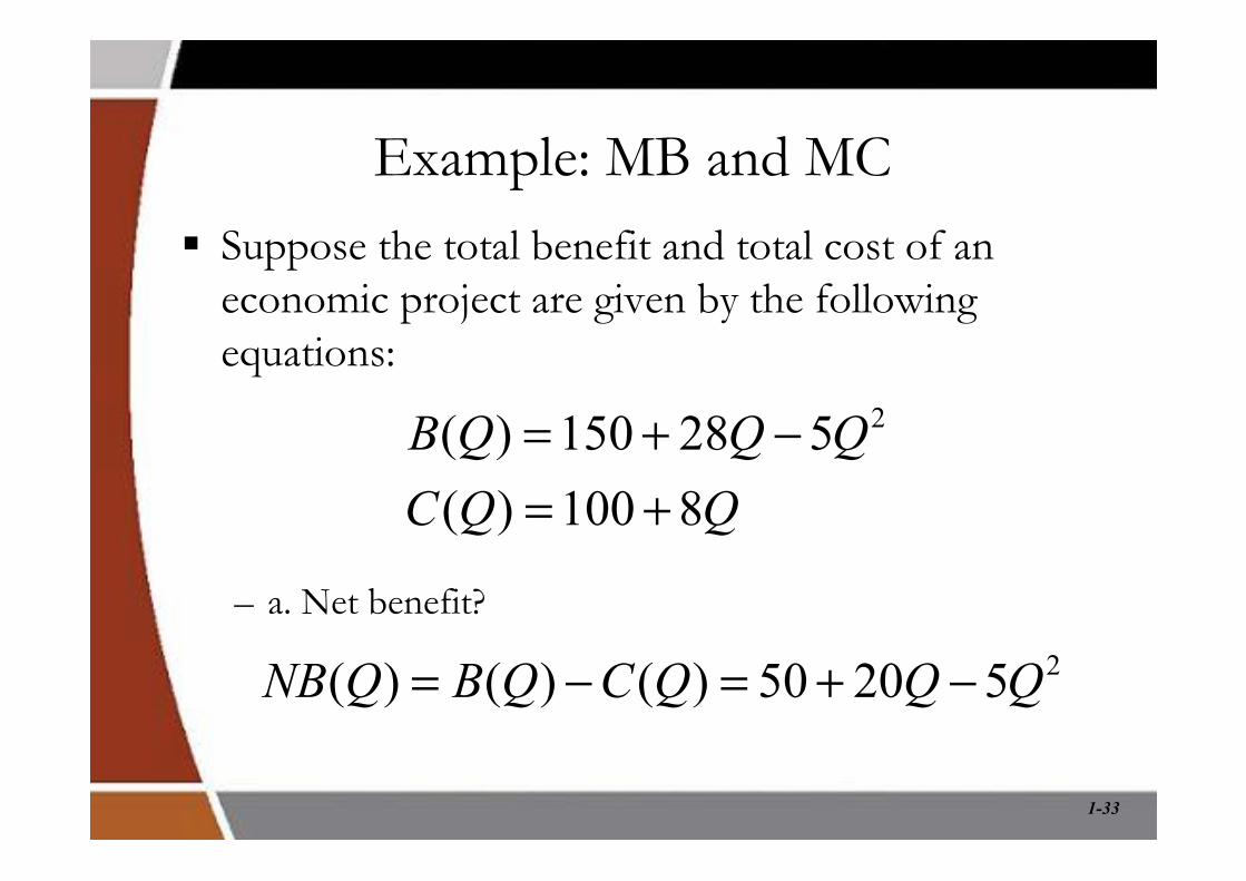
Example: MB and MC §  Suppose the total benefit and total cost of an

economic project are given by the following equations:

–  a. Net benefit?

B(Q) =150+ 28Q −5Q2

C(Q) =100+8Q

NB(Q) = B(Q) −C(Q) = 50+ 20Q −5Q2

1-34

Example: MB and MC

–  a. Marginal benefit?

–  b. Marginal cost?

–  c. Marginal net benefit?

–  d. Maximized net benefit Q?

MB = dB(Q)dQ

= 28−10Q

MC = dC(Q)dQ

= 8

MNB = dNB(Q)dQ

= 20 −10Q = MB −MC

MNB = 0⇒ 20 −10Q = 0⇒Q* = 2

1-35

Conclusion

§  Make sure you include all costs and benefits when making decisions (opportunity cost).

§  When decisions span time, make sure you are comparing apples to apples (PV analysis).

§  Optimal economic decisions are made at the margin (marginal analysis).