chapter 1 spontaneous pattern formation in primary visual
TRANSCRIPT

Chapter 1
Spontaneous pattern formation in
primary visual cortex
Paul C. Bressloff1 and Jack D. Cowan2
1Department of Mathematics, University of Utah,Salt Lake City, Utah 841122Mathematics Department, University of Chicago,Chicago Il. 60637
1.1 Introduction
The primary visual cortex (V1) is the first cortical area to receive visualinformation transmitted by ganglion cells of the retina via the lateral genic-ulate nucleus (LGN) of the thalmus to the back of the brain (see figure 1.1).A fundamental property of the functional architecture of V1 is an orderlyretinotopic mapping of the visual field onto the surface of cortex, with theleft and right halves of visual field mapped onto the right and left corticesrespectively. Except close to the fovea (centre of the visual field), thismap can be approximated by the complex logarithm (see figure 1.2). LetrR = rR, θR be a point in the visual field represented in polar coordi-nates and let r = x, y be the corresponding point in the cortex givenin Cartesian coordinates. Under the retino-cortical map, r = log rR, θR.Evidently, if we introduce the complex representation of rR, zR = rReiθR
then z = log zR = log rR + iθR = x + iy generates the complex corticalrepresentation. One of the interesting properties of the retino-cortical mapis that the action of rotations and dilatations in the visual field correspondto translations in the x and y directions, respectively, in cortex.
Superimposed upon the retinotopic map are a number of additionalfeature maps reflecting the fact that neurons respond preferentially to stim-uli with particular features [38, 43, 55]. For example, most cortical cellssignal the local orientation of a contrast edge or bar—they are tuned to
1

Introduction 2
Figure 1.1. The visual pathway
a particular local orientation [33]. Cells also show a left/right eye prefer-ence known as ocular dominance and some are also direction selective. Thelatter is illustrated in figure 1.1 where the response of a cell to a movingbar is shown. In recent years much information has accumulated aboutthe distribution of orientation selective cells in V1 [27]. In figure 1.3 isgiven a typical arrangement of such cells, obtained via microelectrodes im-
Figure 1.2. The retino-cortical map generated by the complex logarithm

Introduction 3
Figure 1.3. Orientation tuned cells in layers of V1 which is shown in
cross-section. Note the constancy of orientation preference at each cortical lo-
cation [electrode tracks 1 and 3], and the rotation of orientation preference as
cortical location changes [electrode track 2]. Redrawn from [27].
planted in Cat V1. The first panel shows how orientation preferences rotatesmoothly over the surface of V1, so that approximately every 300µm thesame preference reappears, i.e. the distribution is π–periodic in the orien-tation preference angle. The second panel shows the receptive fields of thecells, and how they change with V1 location. The third panel shows moreclearly the rotation of such fields with translation across V1.
A more complete picture of the two–dimensional distribution1 of bothorientation preference and ocular dominance has been obtained using opti-cal imaging techniques [5, 7, 6]. The basic experimental procedure involvesshining light directly on to the surface of the cortex. The degree of lightabsorption within each patch of cortex depends on the local level of ac-tivity. Thus, when an oriented image is presented across a large part of
1 The cortex is of course three-dimensional since it has non-zero thickness with a dis-tinctive layered structure. However, one find that cells with similar feature preferencestend to arrange themselves in vertical columns so that to a first approximation the lay-ered structure of cortex can be ignored. For example, electrode track 1 in figure 1.3 is avertical penetration of cortex that passes through a single column of cells with the sameorientation preference and ocular dominance.

Introduction 4
the visual field, the regions of cortex that are particularly sensitive to thatstimulus will be differentiated. (An example of optical imaging data isshown in figure 1.5). The basic topography revealed by these methods hasa number of characteristic features [43]: (i) Orientation preference changescontinuously as a function of cortical location except at singularities (orpinwheels). (ii) There exist linear regions, approximately 800 × 800µm2
in area (in macaque monkeys), bounded by singularities, within which iso-orientation regions form parallel slabs. (iii) Iso-orientation slabs tend tocross the borders of ocular dominance stripes at right angles. Singular-ities tend to align with the centers of ocular dominance stripes. Theseexperimental findings suggest that there is an underlying periodicity in themicrostructure of V1 with a period of approximately 1mm (in cats andprimates). The fundamental domain of this periodic tiling of the corticalplane is the hypercolumn [34, 38], which contains two sets of orientationpreferences φ ∈ [0, π), one for each eye, organized around a set of foursingularities (see figure 1.4).
L
R
Figure 1.4. Iso–orientation contours in a hypercolumn. There are two ocular
dominance columns corresponding to left (L) and right (R) eye preference. Each
ocular dominance column contains two orientation singularities or pinwheels. A
dashed ring is drawn around one orientation singularity. Redrawn from [6]
Given the existence of a regularly repeating set of orientation and oc-ular dominance maps, how does such a periodic structure manifest itselfanatomically? Two cortical circuits have been fairly well characterized.There is a local circuit operating at sub-hypercolumn dimensions in whichcells make connections with most of their neighbors in a roughly isotropicfashion [21]. The other circuit operates between hypercolumns, connectingcells with similar functional properties separated by several millimetres ofcortical tissue. Optical imaging combined with labelling techniques hasgenerated considerable information concerning the pattern of connections

Introduction 5
Figure 1.5. Lateral Connections made by a cells in Tree Shrew V1. A radioactive
tracer is used to show the locations of all terminating axons from cells in a central
injection site, superimposed on an orientation map obtained by optical imaging.
(Patches with the same coarse-grained orientation preference are shown in the
same colour – this is purely for visualization purposes). The patchy distribution of
the lateral connections is clearly seen, linking regions of like orientation preference
along a particular visuotopic axis. The local axonal field, on the other hand, is
isotropic and connects all neurons within a neighbourhood (≈ 0.7 mm) of the
injection site. Redrawn from [9].
both within and between hypercolumns [5, 6, 40, 66, 9]. A particularlystriking result concerns the intrinsic lateral connections of V1. The axonsof these connections make terminal arbors only every 0.7 mm or so alongtheir tracks [47, 26], and they seem to connect mainly to cells with simi-lar orientation preferences [40, 66, 9]. In addition, as shown in figure 1.5,there is a pronounced anisotropy of the pattern of such connections: its longaxis runs parallel to a patch’s preferred orientation [26, 9]. Thus differingiso-orientation patches connect to patches in neighbouring hypercolumns indiffering directions. Ongoing studies of feedback connections from points inextrastriate areas back to area V1 [1], show that these connectional fieldsare also distributed in highly regular geometric patterns, having a topo-graphic spread of up to 13mm that is significantly larger than the spreadof intrinsic lateral connections. Stimulation of a hypercolumn via lateralor feedback connections modulates rather than initiates spiking activity[31, 57]. Thus this long-range connectivity is ideally structured to providelocal cortical processes with contextual information about the global natureof stimuli. As a consequence the lateral connections have been invoked toexplain a wide variety of context-dependent visual processing phenomena

The Turing mechanism and its role in cooperative cortical dynamics 6
[28, 24, 16].From the perspective of nonlinear dynamics, there are two very distinct
questions one can ask about the large-scale structure of cortex: (i) how didthe feature maps and connectivity patterns first develop? (ii) what typesof spontaneous and stimulus-driven spatio-temporal dynamics arise in themature cortex? It appears that in both cases the Turing mechanism forspontaneous pattern formation plays a crucial role.
1.2 The Turing mechanism and its role in cooperativecortical dynamics
In 1952 Turing [58] introduced an important set of new ideas concern-ing spontaneous pattern formation. The details are well known, but wewill restate them here by way of providing a context for the rest of thischapter. Turing considered the development of animal coat markings asa problem of pattern formation. He started by introducing the idea thatchemical markers in the skin comprise a system of diffusion–coupled chem-ical reactions among substances called morphogens. Turing introduced thefollowing two–component reaction–diffusion system:
∂c∂t
= f(c) + D∇2c (1.1)
where c is a vector of morphogen concentrations, f is (in general) a non-linear vector function representing the reaction kinetics and D is the (di-agonal) matrix of positive diffusion coefficients. What Turing showed wasthat there can exist two different reactions such that in the absence of dif-fusion (D = 0), c tends to a linearly stable homogeneous state, and whenD = 0, D1 = D2, the homogeneous state becomes unstable and c tends toa spatially inhomogeneous state. This was the now famous diffusion driveninstability.
Wilson and Cowan introduced exactly the same mechanism in a neuralcontext [64, 65]. Here we briefly summarize their formulation. Let aE(r, t)be the activity of excitatory neurons in a given volume element of a slabof neural tissue located at r ∈ R2, and aI(r, t) the correspond activity ofinhibitory neurons. aE and aI can be interpreted as local spatio–temporalaverages of the membrane potentials or voltages of the relevant neuralpopulations. In case neuron activation rates are low they can be shown tosatisfy nonlinear evolution equations of the form:
τ∂aE(r, t)
∂t= − aE(r, t) + τ
∫R2
wEE(r|r′)σE [aE(r′, t)]dr′
− τ
∫R2
wEI(r|r′)σI [aI(r′, t)]dr′ + hE(r, t)

The Turing mechanism and its role in cooperative cortical dynamics 7
τ∂aI(r, t)
∂t= − aI(r, t) + τ
∫R2
wIE(r|r′)σE [aE(r′, t)]dr′
− τ
∫R2
wII(r|r′)σI [aI(r′, t)]dr′ + hI(r, t) (1.2)
where wlm(r|r′) = wlm(|r − r′|) gives the weight per unit volume of allsynapses to the lth population from neurons of the mth population a dis-tance |r − r′| away, σE and σI are taken to be smooth output functions
σ(x) =1τ
11 + e−η(x−κ)
(1.3)
where η determines the slope or sensitivity of the input–output characteris-tics of the population and κ is a threshold, hE and hI are external stimuli,and τ is the membrane time constant.
Eqns. (1.2) can be rewritten in the more compact form:
τ∂al(r, t)
∂t= − al(r, t) + τ
∑m=E,I
∫R2
wlm(|r − r′|)σ[am(r′, t)]dr′
+ hl(r, t) (1.4)
Note that wlE ≥ 0 and wlI ≤ 0.In the case of a constant external input, hl(r) = hl, there exists at
least one fixed point solution al(r) = al of equation (1.4), where
al = τ∑
m=E,I
Wlmσ(am) + hl (1.5)
and Wlm =∫R2 wlm(r)dr. If hl is sufficiently small relative to the threshold
κ then this fixed point is unique and stable. Under the change of coordi-nates al → al−hl, it can be seen that the effect of hl is to shift the thresholdby the amount −hl. Thus there are two ways to increase the excitabilityof the network and thus destabilize the fixed point: either by increasingthe external input hl or reducing the threshold κ. The latter can occurthrough the action of drugs on certain brain stem nuclei which, as we shallsee, provides a mechanism for generating geometric visual hallucinations[22, 11, 12, 14].
The local stability of (aE , aI) is found by linearisation:
∂bl(r, t)∂t
= −bl(r, t) + µ∑
m=E,I
∫R2
wlm(|r − r′|)bm(r′, t)dr′ (1.6)
where bl(r, t) = al(r, t)− al and we have performed a rescaling of the localweights τσ′(al)wlm → µwlm with µ a measure of the degree of networkexcitability. We have also rescaled t in units of the membrane time constant

The Turing mechanism and its role in cooperative cortical dynamics 8
τ . Assuming solutions of the form bl(r, t) = bl(r)e−λt we are left with theeigenvalue problem:
λbl(k) = −bl(k) + µ∑m
Wlm(|k|2)bm(k) (1.7)
where bl(k) and Wlm(|k|2) are, respectively, the Fourier coefficients of bl(r)and wlm(r). This leads to the matrix dispersion relation for λ as a functionof q = |k| given by solutions of the characteristic equation
det([λ + 1]I − µW(q)) = 0 (1.8)
where W is the matrix of Fourier coefficients of the wlm. One can ac-tually simplify the formulation by reducing eqns. (1.4) to an equivalentone–population model:
τ∂a(r, t)
∂t= − al(r, t) + τ
∫R2
w(|r − r′|)σ[a(r′, t)]dr′
+ h(r, t) (1.9)
from which we obtain the dispersion relation λ = −1+µW (q) ≡ λ(q), withW (q) the Fourier transform of w(r).
w(r)
r
W(q)
qqc
(a) (b)
1/µ
Figure 1.6. Neural basis of the Turing mechanism. (a) Mexican hat inter-
action function showing short-range excitation and long-range inhibition. (b)
Fourier transform W (q) of Mexican hat function. There exists a critical param-
eter µc = W (qc)−1 where W (qc) = [maxqW (q)] such that for µc < µ < ∞ the
homogeneous fixed point is unstable.
In either case it is relatively straightforward to set up the conditionsunder which the homogeneous state first loses its stability at µ = µc and ata wave–vector with q = qc = 0. In the case of equation (1.9) the conditionis that W (q) be bandpass. This can be achieved with the “Mexican Hat”function (see figure 1.6):
w(|r|) = (a+
σ+)e−r2/σ2
+ − (a−σ−
)e−r2/σ2− (1.10)

The Turing mechanism and its role in cooperative cortical dynamics 9
the Fourier transform of which is:
W (q) =12(a+e−
14 σ2
+q2 − a−e−14 σ2
−q2). (1.11)
Evidently W (0) = (1/2)(a+ − a−) and W (∞) = 0. It is simple to es-tablish that λ passes through zero at the critical value µc signalling thegrowth of spatially periodic patterns with wavenumber qc, where W (qc) =maxqW (q). Close to the bifurcation point these patterns can be repre-sented as linear combinations of plane waves
b(r) =∑
n
(cneikn·r + c∗ne−ikn·r)
where the sum is over all wave vectors with |kn| = qc and n can be boundedby restricting the solutions to doubly–periodic patterns in R2. Dependingon the boundary conditions various patterns of stripes or spots can beobtained as solutions. Figure 1.7 shows, for example, a late stage in thedevelopment of stripes [62]. Amplitude equations for the coefficients cn canthen be obtained in the usual fashion to determine the linear stability ofthe various solutions. This analysis of the Wilson–Cowan equations wasfirst carried out by Ermentrout and Cowan as part of their theory of visualhallucinations [22], and is an exact parallel of Turing’s original analysis,although he did not develop amplitude equations for the various solutions.
Figure 1.7. A late stage in the spontaneous formation of stripes of neural
activity. See text for details.
Essentially the same analysis can be applied to a variety of problemsconcerning the neural development of the various feature maps and connec-tivity patterns highlighted in § 1.1. Consider, for example, the development

The Turing mechanism and its role in cooperative cortical dynamics 10
of topographic maps from eye to brain [61, 63]. Such maps develop by aprocess which involves both genetic and epigenetic factors. Thus the actualgrowth and decay of connections is epigenetic, involving synaptic plasticity.However the final solution is constrained by genetic factors, which act, soto speak, as boundary conditions. The key insight was provided by vonder Malsburg [60] who showed that pattern formation can occur in a de-veloping neural network whose synaptic connectivity or weight matrix isactivity dependent and modifiable, provided some form of competition ispresent. Thus Haussler and von der Malsburg formulated the topographicmapping problem (in the case of a one-dimensional cortex) as follows [30].Let wrs be the weight of connections from the retinal point r to the corticalpoint s, and w the associated weight matrix. An evolution equation for wembodying synaptic plasticity and competition can then be written as
dwdt
= αJ + βw · C(w) − w · B(αJ + βw · C(w)) (1.12)
where J is a matrix with all elements equal to unity, Crs(x) =∑
r′s′ c(r −r′, s − s′)xr′s′ , and
Brs(x) =12(
1N
∑r′
xr′s +1N
∑s′
xrs′).
One can easily show that w = J is an unstable fixed point of eqn (1.12).Linearising about this fixed point leads to the linear equation:
dvdt
= αv + C(v) − B(v) − B[C(v)] (1.13)
where v = w − J. Since B and C are linear operators, we can rewriteeqn (1.13) in the form:
τdvdt
= −v + τ(I − B)[(I + C)(v)] (1.14)
where the time constant τ = (1 − α)−1. It is not too difficult to see thatthe term (I − B)[(I + C)(v)] is equivalent to the action of an effectiveconvolution kernel of the form:
w(r) = w+(r) − w−(r)
so that eqn. (1.14) can be rewritten in the familiar form:
τ∂v(r, t)
∂t= −v(r, t) + τ
∫R2
w(r − r′)v(r′, t)dr′ (1.15)
where in this case r = r, s and v is a matrix. Once again there is a dis-

The Turing mechanism and its role in cooperative cortical dynamics 11
Figure 1.8. Structure of the weight kernel w(r, s).
persion relation of the form λ = −1+µW (k) ≡ λ(k), where k = k, l and,as in the previous examples, assuming appropriate boundary conditions–inthis case periodic–it is the Fourier transform W (k) that determines whichof the eigenmodes
∑kl
cklei 2π
N (kr+ls),
emerges at the critical wavenumber kc = kc, lc. Figure (1.8) shows theform of w(r, s) in the r − s plane. It will be seen that it is similar to theMexican Hat except that the inhibitory surround is in the form of a cross.This forces the eigenmodes that emerge from the Turing instability to bediagonal in the r − s plane. If the wavenumber is selected so that onlyone wave is present, this corresponds to an ordered retino–cortical map.Figure 1.9 shows details of the emergence of the required mode.
Figure 1.9. Stages in the development of an ordered retinotopic map. A single
stripe develops in the r − s plane
A second example is to be found in models for the development ofocular dominance maps [53]. Let nR(r, t) and nL(r, t) be, respectively,the (normalized) right and left eye densities of synaptic connections to

The Turing mechanism and its role in cooperative cortical dynamics 12
the visual cortex modelled as a two–dimensional sheet. Such densities arepresumed to evolve according to an evolution equation of the form:
∂ul(r, t)∂t
=∑
m=R,L
∫R2
wlm(|r − r′|)σ[um(r′, t)]dr′ (1.16)
where ul = log nl
1−nlsuch that σ(ul) = nl and the coupling matrix w is
given by
w(r) = w(r)(
+1 −1−1 +1
),
With the additional constraint nR +nL = 1, equation (1.16) reduces to theone–dimensional form:
∂uR(r, t)∂t
= 2∫R2
w(|r − r′|)σ[uR(r′, t)]dr′ −∫R2
w(|r′|)dr′. (1.17)
which can be rewritten in terms of the variable nR(r, t) as:
∂nR(r, t)∂t
= nR(r, t)(1 − nR(r, t))
[2∫R2
w(|r − r′|)nR(r′, t)dr′ −∫R2
w(|r′|)dr′]. (1.18)
The fixed points of this equation are easily seen to be nR(r) = 0, 1 andnR(r) = 1
2 . The first two fixed points are stable, however the third fixedpoint is unstable to small perturbations. Linearizing about this fixed pointwe find the dispersion relation λ = 1
2W (|k|). Once again the Fourier trans-form of the interaction kernel w(|r|) controls the emergence of the usualeigenmodes, in this case plane waves of the form eik·r in the cortical plane.Note that the fixed point nR = nL = 1
2 corresponds to the fixed pointuR = uL = 0 which is a point of reflection symmetry for the function σ[u].It is this additional symmetry which results in the emergence of stripesrather than spots or blobs when the fixed point destabilizes.
There are many other examples of the role of the Turing instability invisual neuroscience such as the Marr–Poggio model of stereopsis [41] andthe Swindale model for the development of iso–orientation patches [54].However, all of the neural models involve the same basic mechanism ofcompetition between excitation and inhibition (the Mexican hat form ofinteraction, see figure 1.6), and most have some underlying symmetry thatplays a crucial role in the selection and stability of the resulting patterns.In what follows, we shall develop these ideas further by considering in de-tail our own recent work on spontaneous pattern formation in primaryvisual cortex [11, 12, 14]. In this work we have investigated how correla-tions between the pattern of patchy lateral connections and the underlyingorientation map within V1 (as highlighted in § 1.1) effect the large-scale

The Turing mechanism and its role in cooperative cortical dynamics 13
(I) (II)
(III) (IV)
Figure 1.10. Hallucinatory form constants. (a) funnel and (b) spiral images
seen following ingestion of LSD [redrawn from [50]], (c) honeycomb generated by
marihuana [redrawn from [17]], (d) cobweb petroglyph [redrawn from [44]].
dynamics of V1 idealized as a continuous two-dimensional sheet of interact-ing hypercolumns [11, 12, 14]. We have shown that the patterns of lateralconnection are invariant under the so-called shift-twist action of the planarEuclidean group E(2) acting on the product space R2 × S1. By virtue ofthe anisotropy of the lateral connections (see figure 1.5), this shift-twistsymmetry supports distinct scalar and pseudoscalar group representationsof E(2) [8], which characterize the type of cortical activity patterns thatarise through spontaneous symmetry breaking [11]. Following on from theoriginal work of Ermentrout and Cowan [22], we have used our continuummodel to develop a theory for the generation of geometric visual hallucina-tions, based on the idea that some disturbance such as a drug or flickeringlight can destabilize V1 inducing a spontaneous pattern of cortical activitythat reflects the underlying architecture of V1. These activity patternsare seen as hallucinatory images in the visual field, whose spatial scale isdetermined by the range of lateral connections and the cortical-retinotopicmap. Four examples of common hallucinatory images that are reproducedby our model [11] are shown in figure 1.10. Note the contoured nature

A continuum model of V1 and its intrinsic circuitry 14
of the third and fourth images, which could not have been generated inthe original Ermentrout-Cowan model [22]. Our results suggest that thecircuits in V1 that are normally involved in the detection of oriented edgesand in the formation of contours, are also responsible for the generation ofsimple hallucinations.
1.3 A continuum model of V1 and its intrinsic cir-cuitry
Consider a local population of excitatory (E) and inhibitory (I) cells atcortical position r ∈ R2 with orientation preference φ. We characterizethe state of the population at time t by the real-valued activity variableal(r, φ, t) with l = E, I. As in § 1.2, V1 is treated as an (unbounded) con-tinuous two-dimensional sheet of nervous tissue with the additional sim-plifying assumption that φ and r are independent variables – all possibleorientations are represented at every position. Hence, one interpretationof our model would be that it is a continuum version of a lattice of hyper-columns. An argument for the validity of this continuum model is to notethat the separation of two points in the visual field—visual acuity—(at agiven retinal eccentricity of ro), corresponds to hypercolumn spacing [34],and so to each location in the visual field there corresponds a representationin V1 of that location with finite resolution and all possible orientations.Our large-scale model of V1 takes the form
∂al(r, φ, t)∂t
= − al(r, φ, t) + hl(r, φ, t) (1.19)
+∑
m=E,I
∫R2
∫ π
0
wlm(r, φ|r′, φ′)σ[am(r′, φ′, t)]dφ′
πdr′
which is a generalized version of the Wilson–Cowan equations of nervetissue introduced in § 1.2, with t measured in units of τ . The distributionwlm(r, φ|r′, φ′) represents the strength or weight of connections from theiso-orientation patch φ′ at cortical position r′ to the orientation patch φ atposition r.
Motivated by experimental observations concerning the intrinsic cir-cuitry of V1 (see § 1.1), we decompose w in terms of local connectionsfrom elements within the same hypercolumn, and patchy excitatory lateralconnections from elements in other hypercolumns:
wlm(r, φ|r′, φ′) = wloc(φ|φ′)δ(r − r′) + εwlat(r, φ|r′, φ′)δm,Eβl
(1.20)
where ε is a parameter that measures the weight of lateral relative to localconnections. Observations by [31] suggest that ε is small and therefore

A continuum model of V1 and its intrinsic circuitry 15
that the lateral connections modulate rather than drive V1 activity. Notethat although the lateral connections are excitatory [47, 26], 20% of theconnections in layers II and III of V1 end on inhibitory interneurons, so theoverall action of the lateral connections can become inhibitory, especially athigh levels of activity [31]. The relative strengths of the lateral inputs intolocal excitatory and inhibitory populations are represented by the factorsβl.
The local weight distribution is taken to be homogeneous, that is,
wloc(φ|φ′) = W (φ − φ′) (1.21)
for some π-periodic, even function W . It follows that an isolated hypercol-umn (zero lateral interactions) has internal O(2) symmetry correspondingto rotations and reflections within the ring. In order to incorporate theanisotropic nature of the lateral connections, we further decompose wlat as[12]
wlat(r, φ|r′, φ′) = J(T−φ(r − r′))δ(φ − φ′) (1.22)
where
J(r) =∫ π/2
−π/2
p(η)∫ ∞
−∞g(s)δ(r − seη)dsdη (1.23)
with eη = (cos(η), sin(η)), p(−η) = p(η) and Tφ the rotation matrix
Tφ
(xy
)=
(cos φ − sinφsinφ cos φ
) (xy
).
Such a distribution links neurons with the same orientation and spatialfrequency label, with the function p(η) determining the degree of spatialspread (anisotropy) in the pattern of connections relative to the direction oftheir common orientation preference. The weighting function g(s) specifieshow the strength of interaction varies with the distance of separation. Asimplified schematic representation of the pattern of lateral connections isillustrated for our coupled hypercolumn model in figure 1.11.
Substituting equations (1.20) and (1.22) back into equation (1.19)leads to the evolution equation
∂al(r, φ, t)∂t
= − al(r, φ, t) +∑m
∫Wlm(φ − φ′)σ[am(r′, φ′, t)]
dφ′
π(1.24)
+ εβl
∫ π/2
−π/2
p(η)∫ ∞
−∞g(s)σ[aE(r + seη+φ, φ, t)]dηds + hl(r, φ, t)
If p(η) = 1/π for all η then the weight distribution is isotropic and thesystem (1.24) is equivariant with respect to E(2)×O(2), where E(2) denotes

A continuum model of V1 and its intrinsic circuitry 16
hypercolumn
Figure 1.11. Schematic diagram of a coupled hypercolumn model of V1. It
is assumed that there are isotropic local interactions within a hypercolumn,
and anisotropic lateral interactions between hypercolumns. The latter connect
iso-orientation patches located within some angular distance from the visuo-
topic axis parallel to their (common) orientation preference (as illustrated for
the shaded patches).
the Euclidean group of translations, rotations and reflections in the cortex,and O(2) is the internal symmetry group of an isolated hypercolumn. It isimportant to emphasize that cortical rotations are distinct from rotationsin the visual field (which correspond to vertical translations in cortex),as well as from internal rotations with respect to orientation. When p(η)is non-uniform, the resulting anisotropy breaks both cortical and internalO(2) symmetries. However, full Euclidean symmetry, E(2) = R2+O(2), isrecovered by considering the combined Euclidean action on r, φ, whichintroduces a form of shift-twist symmetry in the plane [18, 11, 12, 67].More specifically, the anisotropic weight distribution (1.22) is invariantwith respect to the following action of the Euclidean group:
s · (r, φ) = (r + s, φ) s ∈ R2
ξ · (r, φ) = (Tξr, φ + ξ) ξ ∈ S1
κ · (r, φ) = (κr,−φ)(1.25)
where κ is the reflection (x1, x2) → (x1,−x2). The corresponding groupaction on a function a : R2 × S → R is given by
γ · a(P ) = a(γ−1 · P ) for all γ ∈ R2+O(2) (1.26)

Orientation tuning and O(2) symmetry 17
and the invariance of wlat(P |P ′) is expressed as
γ · wlat(P |P ′) = wlat(γ−1 · P |γ−1 · P ′) = wlat(P |P ′).
It can be seen that the rotation operation comprises a translation or shiftof the orientation preference label φ to φ + ξ, together with a rotation ortwist of the position vector r by the angle ξ. Such an operation providesa novel way to generate the Euclidean group E(2) of rigid motions in theplane. The fact that the weighting functions are invariant with respect tothis form of E(2) has important consequences for the global dynamics ofV1 in the presence of anisotropic lateral connections [11, 12].
1.4 Orientation tuning and O(2) symmetry
In the absence of lateral connections (ε = 0) each hypercolumn is in-dependently described by the so-called ring model of orientation tuning[52, 3, 4, 42, 10], in which the internal structure of a hypercolumn is ide-laized as a ring of orientation selective cells. That is, equation (1.19) re-duces to
∂al
∂t= −al +
∑m=E,I
Wlm ∗ σ(am) + hl (1.27)
where ∗ indicates a convolution operation
W ∗ f(φ) =∫ π/2
−π/2
W (φ − φ′)f(φ′)dφ′
π(1.28)
Just as in § 1.2 the local stability of (aE , aI) is found by linearizationabout the fixed points al :
∂bl
∂t= −bl + µ
∑m
Wlm ∗ bm (1.29)
where bl(r, φ, t) = al(r, φ, t)− al. Equation (1.29) has solutions of the form
bl(r, φ, t) = Bleλt[z(r)e2inφ + z(r)e−2inφ
](1.30)
where z(r) is an arbitrary (complex) amplitude with complex conjugatez(r), and λ satisfies the eigenvalue equation
(1 + λ)B = µW(n)B (1.31)
Here Wlm(n) is the nth Fourier coefficient in the expansion of the π-periodicweights kernels Wlm(φ):
Wlm(φ) = Wlm(0) + 2∞∑
n=1
Wlm(n) cos(2nφ), l, m = E, I (1.32)

Orientation tuning and O(2) symmetry 18
It follows that
λ±n = −1 + µW±
n (1.33)
for integer n, where
W±n =
12
[WEE(n) + WII(n) ± Σ(n)
](1.34)
are the eigenvalues of the weight matrix with
Σ(n) =√
[WEE(n) − WII(n)]2 + 4WEI(n)WIE(n) (1.35)
The corresponding eigenvectors (up to an arbitrary normalization) are
B±n =
(−WEI(n)
12
[WEE(n) − WII(n) ∓ Σ(n)
])
(1.36)
Equation (1.33) implies that, for sufficiently small µ (low network excitabil-ity), λ±
n < 0 for all n and the homogeneous resting state is stable. However,as µ increases an instability can occur leading to the spontaneous formationof an orientation tuning curve.
For the sake of illustration, suppose that the Fourier coefficients aregiven by the Gaussians
Wlm(n) = αlme−n2ξ2lm/2, (1.37)
with ξlm determining the range of the axonal fields of the excitatory andinhibitory populations. We consider two particular cases.
1 2 3 4 5 6
Wn
n
+
Bulk mode
1 2 3n
Wn+
Tuning
mode
Figure 1.12. Spectrum W+n of local weight distribution with (a) a maximum at
n = 1 (tuning mode) and (b) a maximum at n = 0 (bulk mode).
Orientation tuning and O(2) symmetry 19
Case A If WEE(n) = WIE(n) and WII(n) = WEI(n) for all n, thenW−
n = 0 and
W+n = αEEe−n2ξ2
EE/2 − αIIe−n2ξ2II/2 (1.38)
Suppose that ξII > ξEE and 0 < αII < αEE . As we described in § 1.2 theresulting combination of short range excitation and longer range inhibitiongenerates a Turing instability. Of particular relevance to orientation tuningis the case where W+
n has a unique (positive) maximum at n = 1 (seefigure 1.12a). The homogeneous state then destabilizes at the critical pointµ = µc ≡ 1/W+
1 due to excitation of the eigenmodes b(r, φ, t) = Ba(r, φ, t)with B = (1, 1)T and
a(r, φ, t) = z(r)e2iφ + z(r)e−2iφ = |z(r)| cos(2[φ − φ∗(r)]) (1.39)
with z(r) = |z(r)|e−2iφ∗(r). Since these modes have a single maximumin the interval (−90o, 90o), each hypercolumn supports an activity profileconsisting of a solitary peak centred about φ∗(r) = arg z(r). It can be
-90 -45 0 45 90
0
0.2
0.4
0.6
0.8
1
orientation (deg)
input
output
firingrate
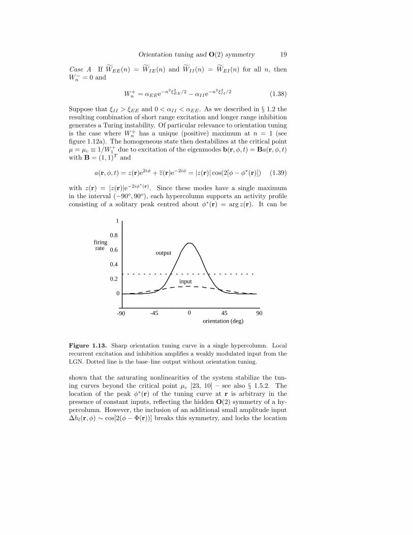
Figure 1.13. Sharp orientation tuning curve in a single hypercolumn. Local
recurrent excitation and inhibition amplifies a weakly modulated input from the
LGN. Dotted line is the base–line output without orientation tuning.
shown that the saturating nonlinearities of the system stabilize the tun-ing curves beyond the critical point µc [23, 10] – see also § 1.5.2. Thelocation of the peak φ∗(r) of the tuning curve at r is arbitrary in thepresence of constant inputs, reflecting the hidden O(2) symmetry of a hy-percolumn. However, the inclusion of an additional small amplitude input∆hl(r, φ) ∼ cos[2(φ − Φ(r))] breaks this symmetry, and locks the location

Amplitude equation for interacting hypercolumns 20
of the tuning curve at each point r to the orientation corresponding to thepeak of the local stimulus, that is, φ∗(r) = Φ(r). As one moves further awayfrom the point of instability, the amplitude of the tuning curve increasesand sharpening occurs due to the nonlinear effects of the firing rate function(1.3). This is illustrated in figure 1.13, where the input and output (nor-malized) firing rate of the excitatory population of a single hypercolumnare shown. Thus the local intracortical connections within a hypercolumnserve both to amplify and sharpen a weakly oriented input signal from theLGN [52, 4]. On the other hand, if the local level of inhibition is reducedsuch that αII αEE , then W+
n is a monotonically decreasing function of|n| (see figure 1.12b), and the homogeneous fixed point undergoes a bulkinstability resulting in broadening of the tuning curve. This is consistentwith experimental data demonstrating a loss of stable orientation tuningin cats with blocking of intracortical inhibition [45]2.
Case B If Σ(n) is pure imaginary, Σ(n) = iΩ(n), then
W±n = αEEe−n2ξ2
EE/2 − αIIe−n2ξ2II/2 ± iΩ(n) (1.40)
Assume, as in case A, that the difference of Gaussians has a maximum atn = 1. Then an instability will occur at the critical point µc = 1/(W+
1 )due to excitation of the oscillatory eigenmodes
b(r, φ, t) =[zL(r)ei(Ω0t−2φ) + zR(r)ei(Ω0t+2φ)
]B + c.c. (1.41)
where Ω0 = µcΩ(1) and B = B+1 . It is then possible for rotating tuning
curves to be generated spontaneously within a hypercolumn [4].
1.5 Amplitude equation for interacting hypercolumns
An isolated hypercolumn exhibits spontaneous O(2) symmetry breakingleading to the formation of an orientation tuning curve. How is this pro-cess modulated by anisotropic lateral interactions between hypercolumns?In this section we use perturbation theory to derive a dynamical equationfor the complex amplitude z(r) for orientation tuning in the presence of lat-eral interactions. We will then use this amplitude equation to show how thelateral interactions induce correlations between z(r) at different points in
2 The idea that local cortical interactions play a role in orientation tuning is still con-troversial. The classical model of Hubel and Wiesel [32] proposes a very different mech-anism, in which both the orientation preference and tuning of a cell arise primarily fromthe geometrical alignment of the receptive fields of the LGN neurons projecting to it.This has also received recent experimental support [25]. On the other hand, intracellu-lar measurements indicate that direct inputs from the LGN to neurons in layer 4 of V1provide only a fraction of the total excitatory inputs relevant to orientation tuning [59]

Amplitude equation for interacting hypercolumns 21
the cortex, leading to spatially periodic patterns of activity across V1 (see§ 1.6). These patterns reproduce the commonly found types of geometricvisual hallucinations when mapped back into visual field coordinates underthe retino cortical map of figure 1.2 (see § 1.6.4). Our basic assumptions inthe derivation of the amplitude equation are as follows: (i) each hypercol-umn is close to a bifurcation point signalling the onset of sharp orientationtuning and (ii) the interactions between hypercolumns are weak.
1.5.1 Cubic amplitude equation: stationary case
Let us perform a Taylor expansion of equation (1.24) with bl(r, φ, t) =al(r, φ, t) − al
∂bl
∂t= − bl +
∑m=E,I
Wlm ∗[µbm + γmb2
m + γ′mb3
m + . . .]+ ∆hl
+ εβlwlat ([σE + µbE + . . .]) (1.42)
where ∆hl = hl − hl and µ = σ′(aE), γl = σ′′(al)/2, γ′l = σ′′′(al)/6. The
convolution operation ∗ is defined by equation (1.28)) and
[wlat f ](r, φ) =∫ π/2
−π/2
∫ ∞
−∞p(η)g(s)f(r + seη+φ, φ)dsdη (1.43)
for an arbitrary function f(r, φ) and wlat given by equation (1.22). Supposethat the system is ε-close to the point of marginal stability of the homoge-neous fixed point associated with excitation of the modes e±2iφ. That is,take µ = µc + ε∆µ where µc = 1/W+
1 , see equation (1.33). Substitute intoequation (1.42) the perturbation expansion
bm = ε1/2b(1)m + εb(2)
m + ε3/2b(3)m + . . . (1.44)
Finally, introduce a slow time-scale τ = εt and collect terms with equalpowers of ε. This leads to a hierarchy of equations of the form (up toO(ε3/2))
[Lb(1)]l = 0 (1.45)
[Lb(2)]l = v(2)l (1.46)
≡∑
m=E,I
γmWlm ∗ [b(1)m ]2 + βlσEwlat 1
[Lb(3)]l = v(3)l (1.47)
≡ − ∂b(1)l
∂τ+
∑m=E,I
Wlm ∗[∆µb(1)
m + γ′m[b(1)
m ]3 + 2γmb(1)m b(2)
m
]
+ µcβlwlat b(1)E + ∆hl
Amplitude equation for interacting hypercolumns 22
with the linear operator L defined according to
[Lb]l = bl − µc
∑m=E,I
Wlm ∗ bm (1.48)
We have also assumed that the modulatory external input is O(ε3/2) andrescaled ∆hl → ε3/2∆hl
The first equation in the hierarchy, equation (1.45), has solutions ofthe form
b(1)(r, φ, τ) =(z(r, τ)e2iφ + z(r, τ) e−2iφ
)B (1.49)
with B ≡ B+1 defined in equation (1.36). We obtain a dynamical equation
for the complex amplitude z(r, τ) by deriving solvability conditions forthe higher order equations. We proceed by taking the inner product ofequations (1.46) and (1.47) with the dual eigenmode b(φ) = e2iφB where
B =(
WIE(1)− 1
2 [WEE(1) − WII(1) − Σ(1)]
)(1.50)
so that[LT b]l ≡ bl − µc
∑m=E,I
Wml ∗ bm = 0
The inner product of any two vector-valued functions of φ is defined as
〈u|v〉 =∫ π
0
[uE(φ)vE(φ) + uI(φ)vI(φ)]dφ
π(1.51)
With respect to this inner product, the linear operator L satisfies 〈b|Lb〉 =〈LT b|b〉 = 0 for any b. Since Lb(p) = v(p), we obtain a hierarchy ofsolvability conditions 〈b|v(p)〉 = 0 for p = 2, 3, . . ..
It can be shown from equations (1.43), (1.46) and (1.49) that the firstsolvability condition is identically satisfied (provided that the system isbifurcating from a uniform state). The solvability condition 〈b|v(3)〉 = 0generates a cubic amplitude equation for z(r, τ). As a further simplificationwe set γm = 0, since this does not alter the basic structure of the amplitudeequation. Using equations (1.43), (1.47) and (1.49) we then find that (afterrescaling τ)
∂z(r, τ)∂τ
= z(r, τ)(∆µ − A|z(r, τ)|2) + f(r) (1.52)
+ β
∫ π
0
wlat [z(r, τ) + z(r, τ)e−4iφ
] dφ
π
where
f(r) = µc
∑l=E,I
Bl
∫ π
0
e−2iφ∆hl(r, φ)dφ
π(1.53)

Amplitude equation for interacting hypercolumns 23
and
β =µ2
cBE
BT B
∑l=E,I
βlBl, A = − 3
BT B
∑l=E,I
Blγ′lB
3l (1.54)
Equation (1.52) is our reduced model of weakly interacting hypercolumns.It describes the effects of anisotropic lateral connections and modulatoryinputs from the LGN on the dynamics of the (complex) amplitude z(r, τ).The latter determines the response properties of the orientation tuningcurve associated with the hypercolumn at cortical position r. The cou-pling parameter β is a linear combination of the relative strengths of thelateral connections innervating excitatory neurons and those innervating in-hibitory neurons with DE , DI determined by the local weight distribution.Since DE > 0 and DI < 0, we see that the effective interactions betweenhypercolumns have both an excitatory and an inhibitory component.
1.5.2 Orientation tuning revisited
In the absence of lateral interactions, equation (1.52) reduces to
∂z(r, τ)∂τ
= z(r, τ)(∆µ − A|z(r, τ)|2) + f(r) (1.55)
For the nonlinear output function (1.3), we find that A > 0. Hence, iff(r) = 0 then there exist (marginally) stable time-independent solutionsof the form z(r) =
√∆µ/Ae−iφ(r) where φ(r) is an arbitrary phase that
determines the location of the peak of the tuning curve at position r. Nowconsider the effects of a weakly biased input from the LGN hl(r, φ, τ) =C(r) cos(2[φ−ωτ ]). This represents a slowly rotating stimulus with angularvelocity ω and contrast C(r) = O(ε3/2). Equation (1.53) implies thatf(r) = C(r)e−2iωτ . Writing z = ve−2i(φ+ωτ) we obtain from (1.55) thepair of equations
v = v(µ − µc + Av2) + C cos(2φ)
φ = − ω − C
2vsin(2φ) (1.56)
Thus, provided that ω is sufficiently small, equation (1.56) will have stablefixed point solution v∗(r), φ∗(r) in which the peak of the tuning curve isentrained to the signal. That is, writing b(1)(r, φ) = Ba(r, φ),
a(r, φ) = v∗(r) cos(2[φ − ωτ − φ∗(r)]) (1.57)
with φ∗(r) = 0 when ω = 0.It is also possible to repeat our bifurcation analysis in the case where
each hypercolumn undergoes a bulk instability. This occurs, for example,

Amplitude equation for interacting hypercolumns 24
when the spectrum of local connections is as in figure 1.12b. The amplitudeequation (1.52) now takes the form
∂a(r, τ)∂τ
= a(r, τ)(∆µ − Aa(r, τ)2) + f0(r) + β
∫ π
0
wlat a(r, τ)dφ
π
(1.58)
with a real and f0 the φ-averaged LGN input. It follows that, in the absenceof lateral interactions, each hypercolumn bifurcates to a φ-independentstate whose amplitude a(r) is a root of the cubic
a(r)(∆µ − Aa(r)2) + f0(r) = 0 (1.59)
1.5.3 Cubic amplitude equation: oscillatory case
In our derivation of the amplitude equation (1.52) we assumed that the localcortical circuit generates a stationary orientation tuning curve. However, asshown in § 1.4, it is possible for a time-periodic tuning curve to occur when(W+
1 ) = 0. Taylor expanding (1.24) as before leads to the hierarchy ofequations (1.45)–(1.47) except that the linear operator L → Lt = L+∂/∂t.The lowest order solution (1.49) now takes the form
b(1)(r, φ, t, τ) =[zL(r, τ)ei(Ω0t−2φ) + zR(r, τ)ei(Ω0t+2φ)
]B + c.c.(1.60)
where zL and zR represent the complex amplitudes for anti-clockwise (L)and clockwise (R) rotating waves (around the ring of a single hypercolumn),and Ω0 = µc(Σ(1)). Introduce the generalized inner product
〈u|v〉 = limT→∞
1T
∫ T/2
−T/2
∫ π
0
[uE(φ, t)vE(φ, t) + uI(φ, t)vI(φ, t)]dφ
πdt
(1.61)
and the dual vectors bL = Bei(Ω0t−2φ), bR = Bei(Ω0t+2φ). Using thefact that 〈bL|Ltb〉 = 〈bR|Ltb〉 = 0 for arbitrary b we obtain the pair ofsolvability conditions 〈bL|v(p)〉 = 〈bR|v(p)〉 = 0 for each p ≥ 2.
As in the the stationary case, the p = 2 solvability conditions areidentically satisfied. The p = 3 solvability conditions then generate cubicamplitude equations for zL, zR of the form
∂zL(r, τ)∂τ
= (1 + iΩ0)zL(r, τ)(∆µ − A|zL(r, τ)|2 − 2A|zR(r, τ)|2)
+ β
∫ π
0
wlat [zL(r, τ) + zR(r, τ)e4iφ
] dφ
π(1.62)

Cortical pattern formation and E(2) symmetry 25
and∂zR(r, τ)
∂τ= (1 + iΩ0)zR(r, τ)(∆µ − A|zR(r, τ)|2 − 2A|zL(r, τ)|2)
+ β
∫ π
0
wlat [zR(r, τ) + zL(r, τ)e−4iφ
] dφ
π(1.63)
where
f±(r) = limT→∞
µc
T
∫ T/2
−T/2
∫ π
0
e−i(Ω0t±2φ)∑
l=E,I
Bl∆hl(r, φ, t)dφ
πdt
(1.64)
Note that the amplitudes only couple to time-dependent inputs from theLGN.
1.6 Cortical pattern formation and E(2) symmetry
We now use the amplitude equations derived in § 1.5 to investigate howO(2) symmetry breaking within a hypercolumn is modified by the presenceof anisotropic lateral interactions, and show how it leads to the formationof spatially periodic activity patterns across the cortex that break the un-derlying E(2) symmetry. We begin by considering the case of stationarypatterns. Oscillatory patterns will be considered in § 1.6.5.
1.6.1 Linear stability analysis
Since we are focusing on spontaneous pattern formation, we shall assumethat there are no inputs from the LGN, f(r) = 0. Equation (1.52) thenhas the trivial solution z = 0. Linearizing about this solution gives
∂z(r, τ)∂τ
= ∆µ z(r, τ) + β
∫ π
0
wlat [z(r, τ) + z(r, τ)e−4iφ
] dφ
π
(1.65)
If we ignore boundary effects by treating V1 as an unbounded two dimen-sional sheet, then equation (1.65) has two classes of solution, z±, of theform
z+(r, τ) = eλ+τe−2iϕ[ceik.r + ce−ik.r
](1.66)
z−(r, τ) = ieλ−τe−2iϕ[ceik.r + ce−ik.r
](1.67)
where k = q(cos(ϕ), sin(ϕ)) and c is an arbitrary complex amplitude. Sub-stitution into equation (1.65) and using equation (1.43) leads to the eigen-value equation
λ± = ∆µ + β
∫ π
0
[∫ ∞
−∞g(s)eiqs cos(φ)ds
] (1 ± χe−4iφ
) dφ
π(1.68)

Cortical pattern formation and E(2) symmetry 26
where
χ =∫ π/2
−π/2
p(η)e−4iηdη (1.69)
Using an expansion in terms of Bessel functions
eix cos(φ) =∞∑
n=−∞(−i)nJn(x)einφ (1.70)
the eigenvalue equation reduces to the more compact form
λ± = ∆µ + βG±(q) (1.71)
withG±(q) = G0(q) ± χG2(q) (1.72)
and
Gn(q) = (−1)n
∫ ∞
−∞g(s)J2n(qs)ds (1.73)
Before using equation (1.71) to determine how the lateral interactionsmodify the condition for marginal stability, we need to specify the formof the weight distribution g(s). From experimental data based on tracerinjections it appears that the patchy lateral connections extend several mmon either side of a hypercolumn and the field of axon terminals within apatch tends to diminish in size the further away it is from the injectionsite [47, 26, 66, 40]. The total extent of the connections depends on theparticular species under study. In our continuum model we assume that
g(s) = e−(s−s0)2/2ξ2
Θ(s − s0) (1.74)
where ξ determines the range and s0 the minimum distance of the (non-local) lateral connections. Recall that there is growing experimental evi-dence to suggest that lateral connections tend to have an inhibitory effectin the presence of high contrast visual stimuli but an excitatory effect at lowcontrasts [28]. It is possible that during the experience of hallucinationsthere are sufficient levels of activity within V1 for the inhibitory effectsof the lateral connections to predominate. Many subjects who have takenLSD and similar hallucinogens report seeing bright white light at the centreof the visual field which then explodes into a hallucinatory image in about3 sec, corresponding to a propagation velocity in V1 of about 2.5 cm persec. suggestive of slowly moving epileptiform activity [50]. In light of this,we assume that β < 0 during the experience of a visual hallucination.
In figure 1.14(a) we plot G±(q) as a function of q for the given weightdistribution (1.74) and the spread function p(η) = δ(η) for which χ = 1.

Cortical pattern formation and E(2) symmetry 27
4 6 8 10
1.2
0.8
0.2
-0.2
2 4 6 8 10
1
0.5
-0.5q
G–(q)G–(q)
q
(a) (b)
q+
q-
2
Figure 1.14. (a) Plot of functions G−(q) (solid line) and G+(q) (dashed line)
in the case χ = 1 (strong anisotropy) and g(s) defined by (1.74) for ξ = 1 and
s0 = 1. The critical wavenumber for spontaneous pattern formation is q−. The
marginally stable eigenmodes are odd functions of φ. (b) Same as (a) except that
χ = sin 4η0/4η0 with lateral spread of width η0 = π/3. The marginally stable
eigenmodes are now even functions of φ.
It can be seen that G±(q) has a unique minimum at q = q± = 0 andG−(q−) < G+(q+). Since β < 0 it follows that the homogeneous statez(r, τ) = 0 becomes marginally stable at the modified critical point µ′
c =µc − εβG−(q−). The corresponding marginally stable modes are given bycombining equations (1.49) and (1.67) for λ− = 0. Writing b(1)(r, φ) =a(r, φ)B we have
a(r, φ) =N∑
n=1
cneikn.r sin(φ − ϕn) + c.c. (1.75)
where kn = q−(cos ϕn, sinϕn) and cn is a complex amplitude. These modeswill be recognized as linear combinations of plane waves modulated by odd(phase-shifted) π-periodic functions sin[2(φ−ϕn)]. The infinite degeneracyarising from rotation invariance means that all modes lying on the circle|k| = q− become marginally stable at the critical point. However, this canbe reduced to a finite set of modes by restricting solutions to be doublyperiodic functions as explained in § 1.6.2.
The solutions (1.75) are precisely the lowest-order odd eigenfunctionsderived using the perturbation methods of [11].3 It is also possible for even(+) eigenmodes to destabilize first when there is a sufficient spread in the
3 Note that in [11] we used a different perturbation scheme in which the strength oflateral connections ε and the distance from the bifurcation point µ − µc were takento be two independent parameters. The linearized equations were first solved using aperturbation expansion in the coupling. Amplitude equations for the linear modes werethen derived by carrying out a Poincare-Linstedt expansion with respect to µ−µc. Thisapproach is particularly suitable for studying the role of symmetries in the spontaneousformation of cortical activity patterns underlying visual hallucinations.

Cortical pattern formation and E(2) symmetry 28
distribution of lateral connections about the visuotopic axis as shown infigure 1.11. More specifically, if we take p(η) = Θ(|η| − η0)/2η0, then
G±(q) = G0(q) ±sin(4η0)
4η0G2(q) (1.76)
such that G+(q+) < G−(q−) when η0 > π/4, which is illustrated in figure1.14(b). It follows that the homogeneous state now becomes marginallystable at the critical point µ′
c = µc − εβG+(q+) due to excitation of theeven modes given by equations (1.49) and (1.66) for λ+ = 0:
a(r, φ) =N∑
n=1
cneikn.r cos(φ − ϕn) + c.c. (1.77)
where kn = q+(cos(ϕn), sin(ϕn)).A third class of solution can occur when each hypercolumn undergoes a
bulk instability, as described by the amplitude equation (1.58). Repeatingthe above linear analysis, we find that there are now only even eigenmodes,which are φ-independent (to leading order), and take the form
a(r) =N∑
n=1
[cneikn.r + cne−ikn.r] (1.78)
The corresponding eigenvalue equation is
λ = ∆µ + G0(q) (1.79)
with G0(q) defined in equation (1.73). Thus |kn| = q0 where q0 is theminimum of G0(q).
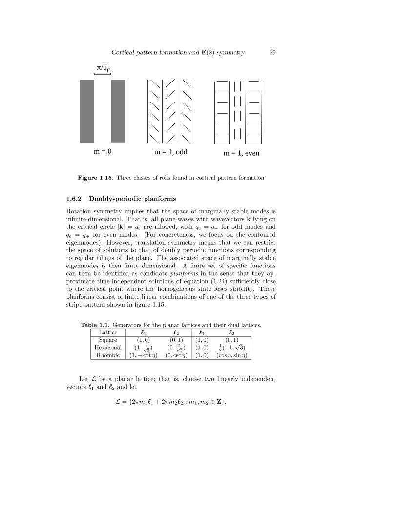
It follows from our analysis that there are three classes of eigenmodethat can bifurcate from the resting state. These are represented, respec-tively, by linear combinations of one of the three classes of roll patternshown in figure 1.15. The m = 0 roll corresponds to modes of the form(1.78), and consists of alternating regions of high and low cortical activityin which individual hypercolumns do not amplify any particular orienta-tion: the resulting patterns are said to be non-contoured. The m = 1rolls correspond to the odd and even oriented modes of equations (1.75)and (1.77). These are constructed using a winner-take-all rule in whichonly the orientation with maximal response is shown at each point in thecortex (after some coarse-graining). The resulting patterns are said to becontoured. The particular class that is selected depends on the detailedstructure of the local and lateral weights. The m = 0 type will be selectedwhen the local inhibition within a hypercolumn is sufficiently weak, whereasthe m = 1 type will occur when there is strong local inhibition, with thedegree of anisotropy in the lateral connections determining whether thepatterns are even or odd.
Cortical pattern formation and E(2) symmetry 29
m = 0 m = 1, odd m = 1, even
π/qc
Figure 1.15. Three classes of rolls found in cortical pattern formation
1.6.2 Doubly-periodic planforms
Rotation symmetry implies that the space of marginally stable modes isinfinite-dimensional. That is, all plane-waves with wavevectors k lying onthe critical circle |k| = qc are allowed, with qc = q− for odd modes andqc = q+ for even modes. (For concreteness, we focus on the contouredeigenmodes). However, translation symmetry means that we can restrictthe space of solutions to that of doubly periodic functions correspondingto regular tilings of the plane. The associated space of marginally stableeigenmodes is then finite–dimensional. A finite set of specific functionscan then be identified as candidate planforms in the sense that they ap-proximate time-independent solutions of equation (1.24) sufficiently closeto the critical point where the homogeneous state loses stability. Theseplanforms consist of finite linear combinations of one of the three types ofstripe pattern shown in figure 1.15.
Table 1.1. Generators for the planar lattices and their dual lattices.
Lattice 1 2 1 2
Square (1, 0) (0, 1) (1, 0) (0, 1)
Hexagonal (1, 1√3) (0, 2√
3) (1, 0) 1
2(−1,
√3)
Rhombic (1,− cot η) (0, csc η) (1, 0) (cos η, sin η)
Let L be a planar lattice; that is, choose two linearly independentvectors 1 and 2 and let
L = 2πm11 + 2πm22 : m1, m2 ∈ Z.

Cortical pattern formation and E(2) symmetry 30
Note that L is a subgroup of the group of planar translations. A functionf :→ R is doubly periodic with respect to L if
f(x + , φ) = f(x, φ)
for every ∈ L. Let θ be the angle between the two basis vectors 1 and2. We can then distinguish three types of lattice according to the valueof θ: square lattice (θ = π/2), rhombic lattice (0 < θ < π/2, θ = π/3) andhexagonal (θ = π/3). After rotation, the generators of the planar latticesare given in table 1.1. Also shown are the generators of the dual latticesatisfying i.j = δi,j with |i| = 1.
D6 D4 D2
Figure 1.16. Holohedries of the plane
Imposing double periodicity means that the original Euclidean sym-metry group is restricted to the symmetry group ΓL of the lattice L. Inparticular, there are only a finite number of shift-twists and reflections toconsider for each lattice (modulo an arbitrary rotation of the whole plane),which correspond to the so-called holohedries of the plane, see figure 1.16.Consequently the corresponding space of marginally stable modes is nowfinite-dimensional—we can only rotate eigenfunctions through a finite setof angles (for example, multiples of π/2 for the square lattice and multiplesof π/3 for the hexagonal lattice). The marginally stable modes for each ofthe lattices are given in table 1.2.
Table 1.2. Eigenmodes corresponding to shortest dual wave vectors ki = qci.
Here u(φ) = cos(2φ) for even modes and u(φ) = sin(2φ) for odd modes.
Lattice a(r, φ)
Square c1u(φ)eik1·r + c2u(φ − π2)eik2·r + c.c.
Hexagonal c1u(φ)eik1·r + c2u(φ − 2π3
)eik2·r + c3u(φ + 2π3
)e−i(k1+k2)·r + c.c.
Rhombic c1u(φ)eik1·r + c2u(φ − η)eik2·r + c.c.
Cortical pattern formation and E(2) symmetry 31
1.6.3 Selection and stability of patterns
It remains to determine the amplitudes cn of the doubly-periodic solutionsthat bifurcate from the homogeneous state (see table 1.2). We proceedby applying the perturbation method of § 1.5.1 to the amplitude equation(1.52). First, introduce a small parameter ξ determining the distance fromthe point of marginal stability according to ∆µ − ∆µc = ξ2 with ∆µc =−βG−(q−) (∆µc = −βG+(q+)) if odd (even) modes are marginally stable.Note that the parameter ξ is independent of the coupling parameter ε.Also introduce a second slow time-scale τ = ξ2τ . Next substitute the seriesexpansion
z(r, τ) = ξz(1)(r, τ) + ξ2z(2)(r, τ) + ξ3z(3)(r, τ) + . . . (1.80)
into equation (1.52) and collect terms with equal powers of ξ. This gener-ates a hierarchy of equations of the form (up to O(ξ3))
Mz(1) = 0 (1.81)Mz(2) = 0 (1.82)
Mz(3) = z(1)[1 − A|z(1)|2
]− dz(1)
dτ(1.83)
where for any complex function z
Mz = −∆µcz − β
∫ π
0
wlat [z + ze−4iφ
] dφ
π(1.84)
The first equation in the hierarchy has solutions of the form
z(1)(r, τ) = ΓN∑
n=1
e−2iϕn[cn(τ)eikn.r + cn(τ)e−ikn.r
](1.85)
where Γ = 1 for even (+) modes and Γ = i for odd (−) modes (see equations(1.66) and (1.67)). Here N = 2 for the square or rhombic lattice and N = 3for the hexagonal lattice. Also kn = qcn for n = 1, 2 and k3 = −k1 − k2.A dynamical equation for the amplitudes cn(τ) can then be obtained as asolvability condition for the third-order equation (1.83). Define the innerproduct of two arbitrary doubly-periodic functions f(r) and g(r) by
〈f |g〉 =∫
Λ
f(r)g(r)dr (1.86)
where Λ is a fundamental domain of the periodically tiled plane (whosearea is normalized to unity). Taking the inner product of the left-handside of equation (1.83) with fn(r) = eikn.r leads to the following solvabilitycondition
〈fn|e2iϕnMz(3) + Γ2e−2iϕnMz(3)〉 = 0 (1.87)

Cortical pattern formation and E(2) symmetry 32
The factor Γ2 = ±1 ensures that the appropriate marginal stability con-dition λ± = 0 is satisfied by equation (1.71). Finally, we substitute forMz(3) using the right-hand side of equation (1.83) to obtain an amplitudeequation for cn, which turns out to be identical for both odd and evensolutions:
dcn
dτ= cn
1 − γ(0)|c1|2 − 2
∑p=n
γ(ϕn − ϕp)|cp|2 (1.88)
whereγ(ϕ) = [2 + cos(4ϕ)]A (1.89)
We consider solutions of these amplitude equations for each of the basiclattices.
Square or rhombic lattice First, consider planforms corresponding to abimodal structure of the square or rhombic type (N = 2). That is, takek1 = qc(1, 0) and k2 = qc(cos(θ), sin(θ)), with θ = π/2 for the square latticeand 0 < θ < π/2, θ = π/3 for a rhombic lattice. The amplitudes evolveaccording to a pair of equations of the form
dc1
dτ= c1
[1 − γ(0)|c1|2 − 2γ(θ)|c2|2
](1.90)
dc2
dτ= c2
[1 − γ(0)|c2|2 − 2γ(θ)|c1|2
](1.91)
Since γ(θ) > 0, three types of steady state are possible.
(i) The homogeneous state: c1 = c2 = 0.(ii) Rolls: c1 =
√1/γ(0)eiψ1 , c2 = 0 or c1 = 0, c2 =
√1/γ(0)eiψ2 .
(iii) Squares or rhombics: cn =√
1/[γ(0) + 2γ(θ)]eiψn , n = 1, 2.
for arbitrary phases ψ1, ψ2. A standard linear stability analysis shows thatif 2γ(θ) > γ(0) then rolls are stable whereas the square or rhombic patternsare unstable. The opposite holds if 2γ(θ) < γ(0). Note that here stabilityis defined with respect to perturbations with the same lattice structure.Using equation (1.89) we deduce that in the case of a rhombic lattice ofangle θ = π/2, rolls are stable if cos(4θ) > −1/2 whereas θ–rhombics arestable if cos(4θ) < −1/2, that is, if π/6 < θ < π/3; rolls are stable andsquare patterns unstable on a square lattice.
Hexagonal lattice Next consider planforms on a hexagonal lattice withN = 3, ϕ1 = 0, ϕ2 = 2π/3, ϕ3 = −2π/3. The cubic amplitude equationstake the form
dcn
dτ= cn
[1 − γ(0)|cn|2 − 2γ(2π/3)(|cn+1|2 + |cn−1|2)
](1.92)

Cortical pattern formation and E(2) symmetry 33
Table 1.3. Even and odd planforms for hexagonal latticeEven Planform (c1, c2, c3) Odd Planform (c1, c2, c3)
0-hexagon (1, 1, 1) hexagon (1, 1, 1)π-hexagon (1, 1,−1) triangle (i,i,i)
roll (1, 0, 0) roll (1, 0, 0)patchwork quilt (0, 1, 1)
where n = 1, 2, 3mod3. Unfortunately, equation (1.92) is not sufficient todetermine the selection and stability of the steady-state solutions bifurcat-ing from the homogeneous state. One has to carry out an unfolding of theamplitude equation that includes higher-order terms (quartic and quintic)in z, z. One could calculate this explicitly by carrying out a double ex-pansion in the parameters ε and ξ, which is equivalent to the perturbationapproach used by [11]. In addition to generating higher-order terms, onefinds that there is an O(ε) contribution to the coefficients γ(ϕ) such that2γ(2π/3) − γ(0) = O(ε) and, in the case of even planforms, an O(ε) con-tribution to the right-hand side of equation (1.92) of the form ηcn−1cn+1.
µcµ
π-hexagons
0-hexagons
rollsC
RA
µcµ
R
C
PQ
H,T
(a) (b)
Figure 1.17. Bifurcation diagram showing the variation of the amplitude C
with the parameter µ for patterns on a hexagonal lattice. Solid and dashed
curves indicate stable and unstable solutions respectively. (a) Even patterns:
Stable hexagonal patterns are the first to appear (subcritically) beyond the bi-
furcation point. Subsequently the stable hexagonal branch exchanges stability
with an unstable branch of roll patterns due to a secondary bifurcation that gen-
erates rectangular patterns RA. Higher–order terms in the amplitude equation
are needed to determine its stability. (b) Odd patterns: Either hexagons (H)
or triangles (T) are stable (depending on higher–order terms in the amplitude
equation) whereas patchwork quilts (PQ) and rolls (R) are unstable. Secondary
bifurcations (not shown) may arise from higher–order terms.
Cortical pattern formation and E(2) symmetry 34
Considerable information about the bifurcating solutions can be ob-tained using group theoretic methods. First, one can use an importantresult from bifurcation theory in the presence of symmetries, namely, theequivariant branching lemma [29]:when a symmetric dynamical system goesunstable, new solutions emerge that (generically) have symmetries corre-sponding to the axial subgroups of the underlying symmetry group. Asubgroup Σ is axial if the dimension of the space of solutions that are fixedby Σ is equal to one. Thus one can classify the bifurcating solutions byfinding the axial subgroups of the symmetry group of the lattice (up toconjugacy). This has been carried out elsewhere for the particular shift-twist action of the Euclidean group described at the end of § 1.3 [11, 12].The results are listed in table 1.3.
It can be seen that major differences emerge between the even and oddcases. Second, symmetry arguments can be used to determine the general
(I)
(III)
(II)
(IV)
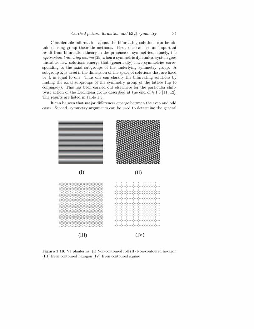
Figure 1.18. V1 planforms. (I) Non-contoured roll (II) Non-contoured hexagon
(III) Even contoured hexagon (IV) Even contoured square

Cortical pattern formation and E(2) symmetry 35
form of higher-order contributions to the amplitude equation (1.92) andthis leads to the bifurcation diagrams shown in figure 1.17 [11, 12]. Itturns out that stability depends crucially on the sign of the O(ε) coeffi-cient 2γ(2π/3) − γ(0), which is assumed to be positive in figure 1.17. Thesubcritical nature of the bifurcation to hexagonal patterns in the case ofeven patterns is a consequence of an additional quadratic term appearingon the right-hand side of (1.92).
1.6.4 From cortical patterns to geometric visual hallucinations
We have now identified the stable planforms that are generated as primarybifurcations from a homogeneous, low activity state of the continuum model(1.24). These planforms consist of certain linear combinations of the rollpatterns shown in figure 1.15 and can thus be classified into non-contoured(m = 0) and contoured (m = 1 even or odd) patterns. Given a particularactivity state in cortex, we can infer what the corresponding image in visual
(I) (II)
(III) (IV)
Figure 1.19. Visual field images of V1 planforms shown in figure 1.18
Cortical pattern formation and E(2) symmetry 36
coordinates is like by applying the inverse of the retino-cortical map shownin figure 1.2. (In the case of contoured patterns, one actually has to specifythe associated tangent map as detailed in [11]). Some examples of stableV1 planforms are presented in figure 1.18 and the associated visual imagesare presented in figure 1.19. It will be seen that the two non-contouredplanforms correspond to the type (I) and (II) Kluver form constants, asoriginally proposed by Ermentrout and Cowan [22], whereas the two con-toured planforms reproduce the type (III) and (IV) form constants (seefigure 1.10).
1.6.5 Oscillating patterns
It is also possible for the cortical model to spontaneously form oscillatingpatterns. This will occur if, in the absence of any lateral connections, eachhypercolumn undergoes a Hopf bifurcation to a time–periodic tuning curvealong the lines described in § 1.5.3. (It is not possible for the lateral con-nections to induce oscillations when the individual hypercolumns exhibitstationary tuning curves. This is a consequence of the fact that the lateralconnections are modulatory and originate only from excitatory neurons).Linearizing equations (1.62) and (1.63) about the zero state zR = zL = 0(assuming zero inputs from the LGN) gives
∂zL(r, τ)∂τ
= ∆µ(1 + iΩ0)zL(r, τ)
+ β
∫ π
0
wlat [zL(r, τ) + zR(r, τ)e4iφ
] dφ
π(1.93)
∂zR(r, τ)∂τ
= ∆µ(1 + iΩ0)zR(r, τ)
+ β
∫ π
0
wlat [zR(r, τ) + zL(r, τ)e−4iφ
] dφ
π(1.94)
Equation (1.93) and (1.94) have solutions of the form
zL(r, τ) = ueλτe2iϕeik.r, zR(r, τ) = veλτe−2iϕeik.r (1.95)
where k = q(cos(ϕ), sin(ϕ)) and λ is determined by the eigenvalue equation
[λ − ∆µ(1 + iΩ0)](
uv
)= β
(G0(q) χG2(q)χG2(q) G0(q)
) (uv
)(1.96)
with Gn(q) given by equation (1.73). Equation (1.96) has solutions of theform
λ± = ∆µ(1 + iΩ0) + βG±(q), v = ±u (1.97)

Cortical pattern formation and E(2) symmetry 37
for G±(q) defined by equation (1.72).Hence, as in the case of stationary patterns, either odd or even time-
periodic patterns will bifurcate from the homogeneous state depending onthe degree of spread in the lateral connections. Close to the bifurcationpoint these patterns are approximated by the eigenfunctions of the lineartheory according to
a(r, φ, t) =N∑
n=1
cos(2[φ − ϕn])[cnei(Ωt+kn.r) + dnei(Ωt−kn.r) + c.c
]
(1.98)
with kn = q+(cos ϕn, sinϕn) for even solutions and
a(r, φ, t) =N∑
n=1
sin(2[φ − ϕn])[cnei(Ωt+kn.r) + dnei(Ωt−kn.r) + c.c.
]
(1.99)
with kn = q−(cos ϕn, sinϕn) for odd solutions, and where Ω = Ω0(1+ε∆µ).These should be compared with the corresponding solutions (1.75) and(1.77) of the stationary case. An immediate consequence of our analysis isthat the oscillating patterns form standing waves within a single hypercol-umn, that is, with respect to the orientation label φ. However, it is possiblefor travelling waves to propagate across V1 if there exist solutions for whichcn = 0, dn = 0 or cn = 0, dn = 0. In order to investigate this possibility,we carry out a perturbation analysis of equations 1.62 and (1.63) along thelines of § 1.6.3 (after the restriction to doubly periodic solutions).
First, introduce a second slow time variable τ = ξ2τ where ξ2 =∆µ − ∆µc and take zL,R = zL,R(r, τ, τ). Next, substitute into equations(1.62) and (1.63) the series expansions
zL,R = ξz(1)L,R + ξ2z
(2)L,R + ξ3z
(3)L,R + . . . (1.100)
and collect terms with equal powers of ξ. This generates a hierarchy ofequations of the form (up to O(ξ3))
[Mτz(p)
]L
= 0,[Mτz(p)
]R
= 0 (1.101)
for p = 1, 2 and
[Mτz(3)
]L
= (1 + iΩ0)z(1)L
[1 − A|z(1)
L |2 − 2A|z(1)R |2
]− ∂z
(1)L
∂τ(1.102)
[Mτz(3)
]R
= (1 + iΩ0)z(1)R
[1 − A|z(1)
R |2 − 2A|z(1)L |2
]− ∂z
(1)R
∂τ(1.103)
Cortical pattern formation and E(2) symmetry 38
where for any z = (zL, zR)
[Mτz]L =∂zL
∂τ− (1 + iΩ0)∆µczL − β
∫ π
0
wlat [zL + zRe+4iφ
] dφ
π
(1.104)
[Mτz]R =∂zL
∂τ− (1 + iΩ0)∆µczR − β
∫ π
0
wlat [zR + zLe−4iφ
] dφ
π
(1.105)
The first equation in the hierarchy has solutions of the form
z(1)L (r, τ, τ) = eiδΩτ
N∑n=1
e2iϕn[cn(τ)eikn.r + dn(τ)e−ikn.r
](1.106)
z(1)R (r, τ, τ) = ΓeiδΩτ
N∑n=1
e−2iϕn[cn(τ)eikn.r + dn(τ)e−ikn.r
](1.107)
where Γ = 1 for even modes and Γ = −1 for odd modes (see equations (1.95)and (1.97)), and δΩ = Ω0∆µc. As in the stationary case we restrict our-selves to doubly periodic solutions with N = 2 for the square or rhombic lat-tice and N = 3 for the hexagonal lattice. A dynamical equation for the com-plex amplitudes cn(τ) and dn(τ) can be obtained as a solvability conditionfor the third-order equations (1.102) and (1.103). Define the inner productof two arbitrary doubly-periodic vectors f(r, τ) = (fL(r, τ), fR(r, τ)) andg(r, τ) = (gL(r, τ), gR(r, τ)) by
〈f |g〉 = limT→∞
1T
∫ T/2
−T/2
∫Λ
[fL(r, τ)gL(r, τ) + fR(r, τ)gR(r, τ)] drdτ
(1.108)
where Λ is a fundamental domain of the periodically tiled plane (whose areais normalized to unity). Taking the inner product of the left-hand sideof equation (1.83) with the vectors fn(r, τ) = eikn.reiδΩτ (e2iϕn ,Γe−2iϕn)and gn(r, τ) = e−ikn.reiδΩτ (e2iϕn ,Γe−2iϕn) leads to the following pair ofsolvability conditions
〈fn|Mτz(3)〉 = 0, 〈gn|Mτz(3)〉 = 0, (1.109)
Finally, we substitute for Mτz(3) using equations (1.102) and (1.103) toobtain amplitude equations for cn and dn (which at this level of approxi-mation are the same for odd and even solutions):
dcn
dτ= − 4(1 + iΩ0)dn
∑p=n
γ(ϕn − ϕp)cpdp + (1 + iΩ0)cn (1.110)
Cortical pattern formation and E(2) symmetry 39
×
1 − 2γ(0)(|cn|2 + 2|dn|2) − 4
∑p=n
γ(ϕn − ϕp)(|cp|2 + |dp|2)
ddn
dτ= − 4(1 + iΩ0)cn
∑p=n
γ(ϕn − ϕp)cpdp + (1 + iΩ0)dn (1.111)
×
1 − 2γ(0)(|dn|2 + 2|cn|2) − 4
∑p=n
γ(ϕn − ϕp)(|cp|2 + |dp|2)
with γ(ϕ) given by equation (1.89).The analysis of the amplitude equations (1.110) and (1.111) is con-
siderably more involved than for the corresponding stationary problem.We discuss only the square lattice here (N = 2) with k1 = qc(1, 0) andk2 = qc(0, 1), The four complex amplitudes (c1, c2, d1, d2) evolve accordingto the set of equations of the form
dc1
dτ= (1 + iΩ0)
(c1
[1 − κ(|c1|2 + 2|d1|2) − 2κ(|c2|2 + |d2|2)
]− 2κd1c2d2
)(1.112)
dc2
dτ= (1 + iΩ0)
(c2
[1 − κ(|c2|2 + 2|d2|2) − 2κ(|c1|2 + |d1|2)
]− 2κd2c1d1
)(1.113)
dd1
dτ= (1 + iΩ0)
(d1
[1 − κ(|c1|2 + 2|d1|2) − 2κ(|c2|2 + |d2|2)
]− 2κc1c2d2
)(1.114)
dd2
dτ= (1 + iΩ0)
(d2
[1 − κ(|c2|2 + 2|d2|2) − 2κ(|c1|2 + |d1|2)
]− 2κd2c1d1
)(1.115)
where κ = 6A. These equations have the same structure as the cubicequations obtained for the standard Euclidean group action using grouptheoretic methods [51]. An identical set of equations has been obtained foroscillatory activity patterns in the Ermentrout-Cowan model [56]. It canbe shown that there exist five possible classes of solution that can bifurcatefrom the homogeneous state. We list examples from each class:
(i) Travelling rolls (TR): c1 = 0, c2 = d1 = d2 = 0 with |c1|2 = 1/κ.(ii) Travelling squares (TS): c1 = c2 = 0, d1 = d2 = 0 with |c1|2 = 1/3κ
Spatial frequency tuning and SO(3) symmetry 40
(iii) Standing rolls (SR): c1 = d1, c2 = d2 = 0 with |c1|2 = 1/3κ(iv) Standing squares (SS): c1 = d1 = c2 = d2 with |c1|2 = 1/9κ(v) Alternating rolls (AR): c1 = −ic2 = d1 = −id2 with |c1|2 = 1/5κ
Up to arbitrary phase-shifts the corresponding planforms are
(TR) a(r, φ, t) = |c1|u(φ) cos(Ωt + qcx)(TS) a(r, φ, t) = |c1| [u(φ) cos(Ωt + qcx) + u(φ − π/2) cos(Ωt + qcy)](SR) a(r, φ, t) = |c1|u(φ) cos(Ωt) cos(qcx)(SS) a(r, φ, t) = |c1| cos(Ωt) [u(φ) cos(qcx) + u(φ − π/2) cos(qcy)](AR) a(r, φ, t) = |c1| [cos(Ωt)u(φ) cos(qcx) + sin(Ωt)u(φ − π/2) cos(qcy)]
(In contrast to the more general case considered by [51], our particularsystem does not support standing cross-roll solutions of the form c1 =d1, c2 = d2 with |c1| = |c2|).
Linear stability analysis shows that (to cubic order) the TR solutionis stable, the AR solution is marginally stable and the other solutions areunstable [51, 56]. In order to resolve the degeneracy of the AR solutionone would need to carry out a double expansion in the parameters ξ, ε andinclude higher order terms in the amplitude equation. The situation iseven more complicated in the case of the hexagonal lattice where such adouble expansion is expected to yield additional contributions to equations(1.110) and (1.111). As in the stationary case, group theoretic methodscan be used to determine generic aspects of the bifurcating solutions. Firstnote that as with other Hopf bifurcation problems the amplitude equationshave an extra phase-shift symmetry in time that was not in the originalproblem. This takes the form ψ : (cn, dn) → (eiψcn, eiψdn) for n = 1, . . . , Nwith ψ ∈ S1. Thus the full spatio-temporal symmetry is ΓL × S1 for agiven lattice L. One can then appeal to the equivariant Hopf theorem [29]which guarantees the existence of primary bifurcating branches that havesymmetries corresponding to the isotropy subgroups of ΓL × S1 with two-dimensional fixed point subspaces. (In the case of a square lattice thisgenerates the five solutions listed above). The isotropy subgroups for thestandard Euclidean group action have been calculated elsewhere [46, 51,20]. As in the stationary bifurcation problem, the isotropy subgroups ofthe shift-twist action may differ in a non-trivial way. This particular issuewill be explored elsewhere.
1.7 Spatial frequency tuning and SO(3) symmetry
One of the simplifications of our large-scale cortical model has been totreat V1 as a continuum of interacting hypercolumns in which the internalstructure of each hypercolumn is idealized as a ring of orientation selectivecells. This reduction can be motivated in part by the fact that there exists

Spatial frequency tuning and SO(3) symmetry 41
a physical ring of orientation domains around each pinwheel, as illustratedby the circle in figure 1.4. However, even if one restricts attention to thesingle eye case, there still exist two pinwheels per ocular dominance column.Moroever, the ring model does not take into account the fact that withineach pinwheel region there is a broad distribution of orientation preferencesso that the average orientation selectivity is weak. A fuller treatment of thetwo-dimensional structure of a hypercolumn can be carried out by incorpo-rating another internal degree of freedom within the hypercolumn, whichreflects the fact that cortical cells are also selective to the spatial frequencyof a stimulus. (In the case of a grating stimulus, this would correspond tothe inverse of the wavelength of the grating). Indeed, recent optical imag-ing data suggests that the two pinwheels per hypercolumn are associatedwith high and low spatial frequencies respectively [7, 36, 37]. Recently, wehave proposed a generalization of the ring model that takes into accountthis structure by incorporating a second internal degree of freedom corre-sponding to (log) spatial frequency preference [15]. Here we show how thisnew model can be used to extend our theory of cortical pattern formationto include both orientation and spatial frequency preferences.
1.7.1 The spherical model of a hypercolumn
Each hypercolumn (when restricted to a single ocular dominance column)is now represented by a sphere with the two orientation singularities iden-tified as the north and south poles respectively (see figure 1.20). Followingrecent optical imaging results [7, 36, 37], the singularities are assumed tocorrespond to the two extremes of (log) spatial frequency within the hy-percolumn. In terms of spherical polar coordinates (r, θ, ϕ) with r = 1,θ ∈ [0, π) and ϕ ∈ [0, 2π), we thus define the orientation preference φ and(log) spatial frequency ν according to
ν = νmin +θ
π[νmax − νmin] , φ = ϕ/2 (1.116)
Note that we consider ν = log p rather than spatial frequency p as a corticallabel. This is motivated by the observation that dilatations in visual fieldcoordinates correspond to horizontal translations in cortex (see § 1.1). Us-ing certain scaling arguments it can then be shown that all hypercolumnshave approximately the same bandwidth in ν even though there is broad-ening with respect to lower spatial frequencies as one moves towards theperiphery of the visual field [15].
It is important to emphasize that the sphere describes the networktopology of the local weight distribution expressed in terms of the internallabels for orientation and spatial frequency. It is not, therefore, expected tomatch the actual spatial arrangement of cells within a hypercolumn. Giventhis spherical topology, the natural internal symmetry of a hypercolumn is

Spatial frequency tuning and SO(3) symmetry 42
νmin
(θ,ϕ)
orientation
spatial frequency
νmax
ν
φ
Figure 1.20. Spherical model of orientation and spatial frequency tuning
now SO(3) rather than O(2). In particular, the local weight distributionis assumed to be SO(3) invariant. Imposing such a symmetry is not just amathematical convenience, but actually reflects the anatomical observationthat the pattern of local interactions within a hypercolumn depends oncortical separation rather than feature separation [19]. When the weightdistribution is expressed in terms of cortical co-ordinates, this naturallyleads to Euclidean symmetry. However, we are describing the interactionsin terms of cortical labels for orientation and spatial frequency. Hence, thenatural measure of spatial separation is now in terms of geodesics or greatcircles on the sphere, and the group that preserves geodesic separation isSO(3).
Having introduced the spherical model of a single hypercolumn, it isstraightforward to write down a generalization of our large-scale corticalmodel given by equation (1.19):
∂a(r, P, t)∂t
= − a(r, P, t) +∫
w(P |P ′)σ[a(r, P ′, t)]dP ′ (1.117)
+ ε
∫wlat(r, P |r′, P ′)σ[a(r′, P ′, t)]dr′dP ′ + h(r, P, t)
where we have introduced the compact notation P = θ, ϕ and dP =sin θdθdϕ. (For ease of notation, we consider here a one-population modelby identifying the states aE = aI . Note that such a state arose previouslyin case A of § 1.4). In equation (1.117), w(P |P ′) denotes the distributionof local connections within a hypercolumn, whereas wlat(r, P |r′, P ′) de-notes the distribution of horizontal connections between the hypercolumns
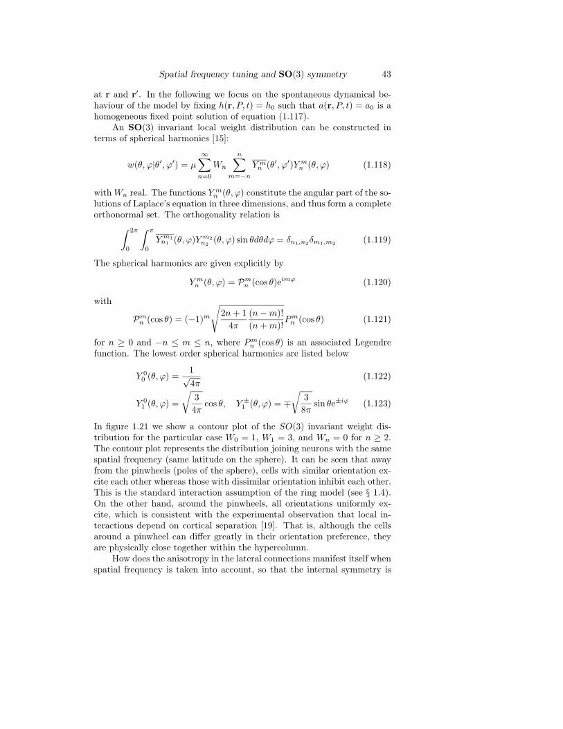
Spatial frequency tuning and SO(3) symmetry 43
at r and r′. In the following we focus on the spontaneous dynamical be-haviour of the model by fixing h(r, P, t) = h0 such that a(r, P, t) = a0 is ahomogeneous fixed point solution of equation (1.117).
An SO(3) invariant local weight distribution can be constructed interms of spherical harmonics [15]:
w(θ, ϕ|θ′, ϕ′) = µ
∞∑n=0
Wn
n∑m=−n
Y mn (θ′, ϕ′)Y m
n (θ, ϕ) (1.118)
with Wn real. The functions Y mn (θ, ϕ) constitute the angular part of the so-
lutions of Laplace’s equation in three dimensions, and thus form a completeorthonormal set. The orthogonality relation is
∫ 2π
0
∫ π
0
Y m1n1 (θ, ϕ)Y m2
n2(θ, ϕ) sin θdθdϕ = δn1,n2δm1,m2 (1.119)
The spherical harmonics are given explicitly by
Y mn (θ, ϕ) = Pm
n (cos θ)eimϕ (1.120)
with
Pmn (cos θ) = (−1)m
√2n + 1
4π
(n − m)!(n + m)!
Pmn (cos θ) (1.121)
for n ≥ 0 and −n ≤ m ≤ n, where Pmn (cos θ) is an associated Legendre
function. The lowest order spherical harmonics are listed below
Y 00 (θ, ϕ) =
1√4π
(1.122)
Y 01 (θ, ϕ) =
√34π
cos θ, Y ±1 (θ, ϕ) = ∓
√38π
sin θe±iϕ (1.123)
In figure 1.21 we show a contour plot of the SO(3) invariant weight dis-tribution for the particular case W0 = 1, W1 = 3, and Wn = 0 for n ≥ 2.The contour plot represents the distribution joining neurons with the samespatial frequency (same latitude on the sphere). It can be seen that awayfrom the pinwheels (poles of the sphere), cells with similar orientation ex-cite each other whereas those with dissimilar orientation inhibit each other.This is the standard interaction assumption of the ring model (see § 1.4).On the other hand, around the pinwheels, all orientations uniformly ex-cite, which is consistent with the experimental observation that local in-teractions depend on cortical separation [19]. That is, although the cellsaround a pinwheel can differ greatly in their orientation preference, theyare physically close together within the hypercolumn.
How does the anisotropy in the lateral connections manifest itself whenspatial frequency is taken into account, so that the internal symmetry is

Spatial frequency tuning and SO(3) symmetry 44
-180o-90o 0o 90o 180o
0o50o
100o150o
-0.8
-0.4
0
0.4
0.8
ϕθ
w
Figure 1.21. Plot of w(θ, ϕ|θ′, ϕ′) given by the SO(3) invariant weight distribu-
tion (1.118) with W0 = 1, W1 = 3 and Wn = 0 for n ≥ 2. Since w only depends
on the difference ϕ − ϕ′, we set ϕ′ = 0 and plot w as a function of θ and ϕ for
θ′ = θ.
SO(3) rather than O(2)? The first point to make is that, unlike O(2),SO(3) does not have a faithful representation in R2. Nevertheless, it ispossible to generalize equation (1.22) so that the weights are invariantwith respect to the action of R2+O(2) = E(2) on r, θ, ϕ. That is, weconsider a lateral weight distribution of the form
wlat(r, P |r′, P ′) = εJ(T−ϕ/2(r − r′))1
sin θ′δ(θ − θ′)δ(ϕ − ϕ′) (1.124)
with J(r) defined by equation (1.23) and ε < 0 (inhibitory lateral inter-actions). Such a distribution links neurons with the same orientation andspatial frequency label, with the function p(η) again determining the degreeof spatial spread (anisotropy) in the pattern of connections relative to thedirection of their common orientation preference. An elegant feature of thespherical model is that it naturally incorporates the fact that, at the popu-lation level, there is less selectivity for orientation near pinwheels. In otherwords, any solution a(r, θ, ϕ) expanded in terms of spherical harmonics isindependent of ϕ at θ = 0, π. This constrains the allowed structure of thespread function p(η), in the sense that the horizontal weight distribution(1.124) has to be isotropic at the pinwheels. This follows from equations(1.124) and (1.23), which show that
∫wlat(r, P |r′, P ′)a(r′, P ′)dP ′

Spatial frequency tuning and SO(3) symmetry 45
=∫ ∞
−∞g(s)
∫ π/2
−π/2
p(η)a(r + srϕ/2+η, P )dηds (1.125)
It is clear that the right-hand of this equation will be independent of ϕ atθ = 0, π if and only if p(η) = 1/π at the pinwheels. In order to incorpo-rate the known anisotropy away from the pinwheels, we conclude that thespread function has to be θ-dependent, p = p(η|θ). An example of a spreadfunction that smoothly interpolates between isotropic connections at thepinwheels (high and low spatial frequencies) and strong anisotropy in thelinear zones (intermediate spatial frequencies) with degree of spread η0 is
p(η|θ) =cos2 θ
π+
12η0
Θ(η0 − |η|) sin2 θ (1.126)
The anisotropic weight distribution (1.124) is invariant under the followingaction of R2+O(2) = E(2) on r, θ, ϕ:
s · (r, θ, ϕ) = (r + s, θ, ϕ) s ∈ R2
ξ · (r, θ, ϕ) = (Tξr, θ, ϕ + ξ) ξ ∈ S1
κ · (r, θ, ϕ) = (κr, θ,−ϕ)(1.127)
where κ is the reflection (x1, x2) → (x1,−x2).
1.7.2 Cortical patterns and spatial frequency tuning
A theory of spontaneous pattern formation in the coupled spherical model(1.117) can be developed along similar lines to that of the coupled ringmodel (1.24). Now each isolated hypercolumn generates a tuning surfacefor orientation and spatial frequency through spontaneous SO(3) symmetrybreaking. The peak of this surface can be locked to a weakly biased stimulusfrom the LGN. Moreover, lateral interactions induce correlations betweenthe tuning surfaces across the cortex leading to spatially periodic patternsof activity, which are consistent with the hallucinatory images presentedin § 1.6.4. Rather than presenting the full nonlinear analysis here, werestrict ourselves to studying the linear eigenmodes that are excited whena homogeneous fixed point of the network becomes unstable.
First, we linearize equation (1.117) about the fixed point solutiona(r, θ, ϕ, t) = a0. Setting a(r, θ, ϕ, t) = a0 + eλtu(θ, ϕ)eik.r generates theeigenvalue equation
λu(P ) = −u(P ) + µ
∫w(P |P ′)u(P ′)dP ′ + εJ(Tϕ/2k)u(P ) (1.128)
where J(k) is the Fourier transform of J(r) and k = q(cos ζ, sin ζ). Ex-panding u(θ, ϕ) in terms of spherical harmonics
u(θ, ϕ) =∑n∈Z
n∑m=−n
e−imζAnmY mn (θ, ϕ) (1.129)

Spatial frequency tuning and SO(3) symmetry 46
leads to the matrix eigenvalue equation
[λ + 1 − µWn]Anm = ε∑n′∈Z
n′∑m′=−n′
Jnm,n′m′(q)An′m′ (1.130)
with
Jnm,n′m′(q) =∫ 2π
0
∫ π
0
Y mn (θ, ϕ)Y m′
n′ (θ, ϕ) (1.131)
×[∫ π/2
π/2
p(η|θ)∫ ∞
0
g(s) cos(sq cos[ϕ/2 + η])dηds
]sin θdθdϕ
We have included an additional phase-factor e−imζ in equation (1.129) thatsimplifies the matrix equation (1.130) by eliminating any dependence onthe direction ζ of the wavevector k. Such a phase factor is equivalent toshifting ϕ, since e−imζY m
n (θ, ϕ) = Y mn (θ, ϕ − ζ).
The matrix elements Jnm,n′m′(q) are evaluated by substituting theexplicit expression (1.120) for the spherical harmonics into equation (1.131):
Jnm,n′m′(q) = 2πGm−m′(q)Γnm,n′m′ (1.132)
where Gm(q) satisfies equation (1.73) and
Γnm,n′m′ =∫ π
0
Pmn (cos θ)Pm′
n′ (cos θ)
[∫ π/2
−π/2
p(η|θ)e2i(m−m′)ηdη
]sin θdθ
(1.133)
For the spread function (1.126) we have
Γnm,n′m′ =∫ π
0
Pmn (cos θ)Pm′
n′ (cos θ) (1.134)
×[δm−m′ cos2 θ +
sin[2(m − m′)η0]2(m − m′)η0
sin2 θ
]sin θdθ
In the absence of lateral interactions (ε = 0), each hypercolumn canexhibit orientation and spatial frequency tuning through spontaneous sym-metry breaking of SO(3). This is a generalization of the O(2) symmetrybreaking mechanism underlying orientation tuning in the ring model (see§ 1.4). The orthogonality relation (1.119) shows that the eigenmodes arespherical harmonics with λ = λn ≡ −1 + µWn for u(θ, ϕ) = Y m
n (θ, ϕ),−n ≤ m ≤ n. Since λ is k-independent, the full solution for the eigen-modes can be written in the form
a(r, θ, ϕ) − a0 = c0(r)Y 0n (θ, ϕ) +
n∑m=1
[cm(r)Y m
n (θ, ϕ) + cm(r)Y mn (θ, ϕ)
]
(1.135)
Spatial frequency tuning and SO(3) symmetry 47
with the coefficients cm(r) arbitrary modulo the normalization condition
n∑m=0
|cm(r)|2 = B (1.136)
where B is fixed. This normalization condition reflects the fact that theassociated amplitude equations for the coefficients cm(r) are SO(3) equiv-ariant [15].
Suppose that W1 > Wn for all n = 1. The fixed point a = a0 thendestabilizes at a critical value of the coupling µc = 1/W1 due to excitationof the first-order spherical harmonics. Sufficiently close to the bifurcationpoint, the resulting activity profile can be written as
a(r, θ, ϕ) = a0 + c0(r) +∑
m=0,±cm(r)fm(θ, ϕ) (1.137)
for real coefficients c0(r), c±(r) with∑
m=0,± cm(r)2 = B and
f0(θ, ϕ) = cos θ, f+(θ, ϕ) = sin θ cos ϕ, f−(θ, ϕ) = sin θ sinϕ (1.138)
Equation (1.137) represents a tuning surface for orientation and spatial fre-quency preferences for the hypercolumn at cortical position r, which con-sists of a solitary peak whose location is determined by the values of thecoefficients (c0(r), c+(r), c−(r)). Such a solution spontaneously breaks theunderlying SO(3) symmetry. However, full spherical symmetry is recov-ered by noting that rotation of the solution corresponds to an orthogonaltransformation of the coefficients c0, c±. Thus the action of SO(3) is toshift the location of the peak of the activity profile on the sphere, thatis, to change the particular orientation and spatial frequency selected bythe tuning surface. (This hidden SO(3) symmetry is explicitly broken byexternal stimuli, along similar lines to § 1.5.2).
The tuning surface generated by our spherical model has the impor-tant property that it is not separable with respect to orientation and spa-tial frequency – the activity profile cannot be written in the form u(θ, ϕ) =Θ(θ)Φ(ϕ). Consequently, selectivity for orientation varies with spatial fre-quency. If c± = 0 then the activity profile is peaked at the pinwheelassociated with high (c0 > 0) or low (c0 < 0) spatial frequencies, andthere is no selection for orientation. On the other hand, if c0 = 0 then theactivity profile is peaked at intermediate spatial frequencies and there isstrong selection for orientation. It is important to emphasize that the tun-ing surface represents the activity profile of a population of cells within ahypercolumn, rather than the tuning properties of an individual cell. Thusthe absence of orientation selectivity at pinwheels is an aggregate propertyof the population. Indeed, it has been found experimentally that individ-ual cells around pinwheels are orientation selective, but there is a broad

Spatial frequency tuning and SO(3) symmetry 48
distribution of orientation preferences within the pinwheel region so thatthe average response of the population is not orientation selective.
In order to solve the eigenvalue equation (1.130) for non-zero ε, we ex-ploit the experimental observation that the lateral connections are weakrelative to the local connections, and carry out a perturbation expan-sion in the small parameter ε. We show that there is a q–dependentsplitting of the degenerate eigenvalue λ1 that also separates out the first-order spherical harmonics. Denoting the characteristic size of such a split-ting by δλ = O(ε), we impose the condition that δλ µ∆W , where∆W = minW1−Wm, m = 1. This ensures that the perturbation does notexcite states associated with other eigenvalues of the unperturbed problem,and we can then restrict ourselves to calculating perturbative correctionsto the degenerate eigenvalue λ1 and its associated eigenfunctions. Thus,introduce the perturbation expansions
λ = −1 + µW1 + ελ(1) + ε2λ(2) + . . . (1.139)
Anm = cmδn,1 + εA(1)nm + ε2A(2)
nm + . . . (1.140)
and substitute these into the eigenvalue equation (1.130). We then system-atically solve the resulting hierarchy of equations to successive orders in ε,taking into account the fact that the unperturbed problem is degenerate.Here we will only describe the lowest order corrections.
Setting n = 1 in equation (1.130) yields the O(ε) equations
1∑m,m′=−1
Jmm′(q)cm′ = λ(1)cm
where Jmm′(q) = J1m,1m′(q). Using equations (1.126), (1.132) and (1.134),we find that
G0(q) 0 00 G0(q) 4χG2(q)/50 4χG2(q)/5 G0(q)
c0
c1
c−1
= λ(1)
c0
c1
c−1
(1.141)
where χ is given by equation (1.69). Equation (1.141) has solutions of theform
λ(1) = λ(1)0 (q) ≡ G0(q) (1.142)
with eigenmode c0 = 1, c± = 0 and
λ(1) = λ(1)± (q) ≡ G0(q) ±
45χG2(q) (1.143)

Future directions 49
with eigenmodes c0 = 0, c−1 = ±c1.As a concrete example, suppose that g(s) is given by equation (1.74)
and χ = sin 4η0/4η0. Plotting Gm(q) for m = 0, 2 establishes that whenthere is sufficiently strong anisotropy in the linear zones (η0 < π/4)
minq
λ(1)− (q) < min
qλ(1)
0 (q) < minq
λ(1)+ (q) (1.144)
and the marginally stables modes are of the form
a(r, θ, ϕ) =∑
i
bieiki.r sin θ sin(ϕ − ζi) (1.145)
where ki = qc(cos ζi, sin ζi) and qc is the wavenumber that minimizesλ
(1)− (q). On the other hand, when there is weaker anisotropy within the
linear zones (η0 > π/4)
minq
λ(1)+ (q) < min
qλ(1)
0 (q) < minq
λ(1)− (q) (1.146)
and the marginally stables modes are now of the form
a(r, θ, ϕ) =∑
i
bieiki.r sin θ cos(ϕ − ζi) (1.147)
In both cases, these are states in which each hypercolumn has a tuningsurface that peaks at intermediate frequencies. This regime is the onerelevant to contour formation, and thus we recover the basic contouredpatterns presented in § 1.6.4.
1.8 Future directions
There are many directions in which this work can be expanded. For ex-ample, it is now clear that many different features are mapped onto thevisual cortex and beyond in addition to retinal position, orientation andspatial frequency. Thus ocularity, directional motion, binocular disparity,and colour seem to be mapped [39, 35, 6, 48, 36]. It therefore remains towork out the symmetry groups associated with these features and thence toapply the mathematical machinery we have introduced above to computethe patterns which arise via spontaneous symmetry breaking.
There is also the fact that the neuron model used to formulate equa-tions (1.4) is extremely simplified. It is nothing more than a low–pass RCfilter followed by a sigmoidal current–voltage characteristic. One can easilymake this model more complex and realistic by adding recovery variablesin the style of the Fitzhugh–Nagumo equations [64], or one can simplify itstill further by using the well–known integrate–and–fire model [10]. Inter-estingly, in either case the dynamics is richer, and a variety of oscillatoryphenomena are immediately apparent.

References 50
However the most interesting new direction is to study, not sponta-neous but driven pattern formation in neural networks of the type we haveintroduced. This amounts to studying the effects of external stimuli onsuch networks. In our case this means studying the effects of visual stim-uli. Depending on the order of magnitude of such stimuli, various effectsare possible. Thus external stimuli of order O(1) couple to the fixed pointsof equation (1.4), stimuli of order O(ε1/2) couple to the linearized equa-tions (1.6), and O(ε3/2) stimuli couple directly to amplitude equations suchas those of equation (1.52) and effectively unfold any bifurcation [10, 13].The various effects produced by these and related stimuli remain to bestudied in detail.
1.9 References
[1] Angelucci A, Levitt J B, Hupe J M, Walton E J S , Bullier J and LundJ S, 2000. Anatomical circuits for local and global integration of visualinformation: Intrinsic and feedback connections. Europ. J. Neurosci. 12285.
[2] Angelucci A, Levitt J B and Lund J S, 2002. Anatomical origins of theclassical receptive field and modulatory surround field of single neurons inmacaque visual cortical area v1. Progress in Brain Research (in press).
[3] Ben-Yishai R, Lev Bar-Or R and Sompolinsky H, 1995 Theory of orientationtuning in visual cortex. Proc. Nat. Acad. Sci. 92 3844-3848
[4] Ben-Yishai R, Hansel D and Sompolinsky H, 1997 Traveling waves and theprocessing of weakly tuned inputs in a cortical network module. J. Comput.Neurosci. 4 57-77
[5] Blasdel G G and Salama G, 1986 Voltage-sensitive dyes reveal a modularorganization in monkey striate cortex. Nature 321 579-585
[6] Blasdel G G, 1992 Orientation selectivity, preference, and continuity in mon-key striate cortex. J. Neurosci. 12 3139-3161
[7] Bonhoeffer T, Kim D S, Malonek D, Shoham D and Grinvald A, 1995 Opticalimaging of the layout of functional domains in area 17/18 border in catvisual cortex. European J. Neurosci. 7 1973-1988
[8] Bosch Vivancos I, Chossat P and Melbourne I, 1995 New planforms in systemsof partial differential equations with Euclidean symmetry. Arch. Rat. Mech.131: 199–224.
[9] Bosking W H, Zhang Y, Schofield B and Fitzpatrick D, 1997 Orientationselectivity and the arrangement of horizontal connections in tree shrewstriate cortex. J. Neurosci. 17 2112-2127.
[10] Bressloff P C, Bressloff N W and Cowan J D, 2000 Dynamical mechanismfor sharp orientation tuning in an integrate–and–fire model of a corticalhypercolumn. Neural Comput. 12 2473-2511
[11] Bressloff P C, Cowan J D, Golubitsky M, Thomas P J and Wiener M, 2001Geometric visual hallucinations, Euclidean symmetry and the functionalarchitecture of striate cortex. Phil. Trans. Roy. Soc. Lond. B 356 299-330
[12] Bressloff P C, Cowan J D, Golubitsky M and Thomas P J, 2001 Scalar and

References 51
pseudoscalar bifurcations: pattern formation on the visual cortex. Nonlin-earity 14 739-775.
[13] Bressloff P C and Cowan J D, 2002 An Amplitude Equation approach toContextual Effects in Visual Cortex. Neural Comput. 14 493-525
[14] Bressloff P C, Cowan J D, Golubitsky M, Thomas P J and Wiener M, 2002What geometric visual hallucinations tell us about the visual cortex. NeuralComput. 14 473-491
[15] Bressloff P C and Cowan J D, 2002 SO(3) symmetry breaking mechanismfor orientation and spatial frequency tuning in visual cortex Phys. Rev.Lett. 88 078102
[16] Bullier J, Hupe′ J-M, James A J and Girard P, 2001 The role of feedbackconnections in shaping the response of visual cortical neurons. Prog. BrainRes. 134 193-204.
[17] Clottes J and Lewis-Williams D, 1998 The Shamans of Prehistory: Tranceand Magic in the Painted Caves. New York: Abrams.
[18] Cowan J D, 1997 Neurodynamics and Brain Mechanisms. In Ito M,Miyashita Y and Rolls E T, editors, Cognition, Computation, and Con-sciousness (Oxford University Press) p. 205-233
[19] Das A and Gilbert C, 1999 Topography of contextual modulations mediatedby short–range interactions in primary visual cortex Nature 399 655-661
[20] Dionne B, Golubitsky M, Silber M and Stewart I, 1995 Time–periodic spa-tially periodic planforms in Euclidean equivariant partial differential eq-narrays. Phil. Trans. Roy. Soc. Lond. A 325 125-168
[21] Douglas R, Koch C, Mahowald M, Martin K and Suarez H, 1995 Recurrentexcitation in neocortical circuits. Science 269 981-985
[22] Ermentrout G B and Cowan J D, 1979 A mathematical theory of visualhallucination patterns. Biol. Cybernetics 34 137-150
[23] Ermentrout G B, 1998 Neural networks as spatial pattern forming systems.Rep. Prog. Phys. 61 353-430
[24] Fitzpatrick D, 2000 Seeing beyond the receptive field in primary visualcortex. Curr. Op. in Neurobiol. 10 438-443
[25] Ferster D, Chung S and Wheat H, 1997 Orientation selectivity of thalamicinput to simple cells of cat visual cortex. Nature 380 249-281
[26] Gilbert C D and Wiesel T N, 1983 Clustered intrinsic connections in catvisual cortex. J. Neurosci. 3 1116-1133
[27] Gilbert C D, 1992 Horizontal integration and cortical dynamics Neuron 91-13
[28] Gilbert C D, Das A, Ito M, Kapadia M and Westheimer G, 1996 Spatialintegration and cortical dynamics. Proc. Nat. Acad. Sci. 93 615-622
[29] Golubitsky M, Stewart I and Schaeffer D G, 1988 Singularities and Groupsin Bifurcation Theory II. (Berlin: Springer–Verlag)
[30] Haussler A and von der Malsburg C 1983 Development of Retinotopic Pro-jections: An Analytical Treatment J. Theoret. Neurobiol. 2 47-73
[31] Hirsch J D and Gilbert C D, 1991 Synaptic physiology of horizontal con-nections in the cat’s visual cortex. J. Physiol. Lond. 160 106-154
[32] Hubel D H and Wiesel T N, 1962 Receptive fields, binocular interaction andfunctional architecture in the cat’s visual cortex. J. Neurosci. 3 1116-1133
[33] Hubel D H and Wiesel T N, 1974a Sequence regularity and geometry of

References 52
orientation columns in the monkey striate cortex. J. Comp. Neurol. 158267-294.
[34] Hubel D H and Wiesel T N, 1974 Uniformity of monkey striate cortex: Aparallel relationship between field size, scatter, and magnification factor.J. Comp. Neurol. 158 295-306.
[35] Hubel D H and Livingstone M S, 1987 Segregation of form, color, andstereopsis in primate area 18. J. Neurosci. 7 3378-3415.
[36] Hubener M, Shoham D, Grinvald A and Bonhoeffer T, 1997 Spatial rela-tionship among thre columnar systems. J. Neurosci. 15 9270-9284.
[37] Issa N P, Trepel C and Stryker M P, 2000. Spatial frequency maps in catvisual cortex. J. Neurosci. 20 8504-8514.
[38] LeVay S and Nelson S B 1991. Columnar organization of the visual cortex.The neural basis of visual function ed Leventhal A G (Boca Raton: CRCPress) pp 266-315
[39] Livingstone M S and Hubel D H, 1984 Anatomy and physiology of a colorsystem in the primate visual cortex. J. Neurosci. 4 309-356.
[40] Malach R, Amir Y, Harel M and Grinvald A, 1993 Relationship betweenintrinsic connections and functional architecture revealed by optical imag-ing and in vivo targeted biocytin injections in primate striate cortex. Proc.Natl. Acad. Sci. 90 10469-10473
[41] Marr D and Poggio T, 1976 Cooperative computation of stereo disparityScience 194 283-287
[42] Mundel T, Dimitrov A and Cowan J D, 1997 Visual cortex circuitry andorientation tuning. In Mozer M C, Jordan M I and Petsche T, editors,Advances in Neural Information Processing Systems, volume 9 (MIT Press)p. 886-893
[43] Obermayer K and Blasdel G G, 1993 Geometry of orientation and oculardominance columns in monkey striate cortex. J. Neurosci. 13 4114-4129
[44] Patterson A, 1992 Rock Art Symbols of the Greater Southwest . Boulder CO:Johnson Books.
[45] Phleger B and Bonds A B, 1995 Dynamic differentiation of gabaA–sensitiveinfluences on orientation selectivity of complex cells in the cat striate cor-tex. Exp. Brain Res. 104
[46] Roberts M, Swift J and Wagner D H, 1986 The Hopf bifurcation on ahexagonal lattice. Contemp. Math. 56 283-318
[47] Rockland K S and Lund J, 1983 Intrinsic laminar lattice connections inprimate visual cortex. J. Comp. Neurol. 216 303-318
[48] Shmuel A and Grinvald A, 1996 Functional Organization for Direction ofMotion and its Relationship to Orientation Maps in Cat Area 18. J. Neu-rosci. 16 6945-6964
[49] Shmuel A, Korman M, Harel M, Grinvald A and Malach R, 1998 Relation-ship of feedback connections from area V2 to orientation domains in areaV1 of the primate. Soc Neurosci. Abstr. 24 767
[50] Siegel R K and Jarvik M E, 1975 Drug-induced hallucinations in animalsand man. In Siegel R K and West L J, editors, Hallucinations: Behavior,Experience and Theory, (New York: Wiley) p. 81-161
[51] Silber M and Knobloch E 1991 Hopf bifurcation on a square lattice. Non-linearity 4 1063-1107

References 53
[52] Somers D C, Nelson S and Sur M, 1995 An Emergent Model of OrientationSelectivity in Cat Visual Cortical Simple Cells. J. Neurosci. 15 5448-5465
[53] Swindale N V, 1980 A model for the formation of ocular dominance stripes.Proc. Roy. Soc. Lond. B 208 243-264
[54] Swindale N V, 1982 A model for the formation of orientation columns Proc.Roy. Soc. Lond. B 215 211-230
[55] Swindale N V, 1996 The development of topography in visual cortex: areview of models Network 7 161-247
[56] Tass P, 1997 Oscillatory cortical activity during visual hallucinations. J.Biol. Phys. 23 21-66
[57] Toth L J, Rao S C, Kim D-S, Somers D C and Sur M, 1996 Subthresholdfacilitation and suppression in primary visual cortex revealed by intrinsicsignal imaging. Proc. Natl. Acad. Sci. 93 9869-9874
[58] Turing A M, 1952 The Chemical Basis of Morphogenesis Phil. Trans. RoySoc. Lond. B 237 32-72
[59] Vidyasagar T R, Pei X and Volgushev M, 1996 Multiple mechanisms un-derlying the orientation selectivity of visual cortical neurons. Trends inNeurosci. 19 272-277
[60] von der Malsburg C, 1973 Self-organization of Orientation Selective cells inthe Striate Cortex. Kybernetik 14 85-100
[61] von der Malsburg C and Willshaw D J, 1977 How to label nerve cells sothat they can interconnect in an ordered fashion. Proc.Natl.Acad.Sci. USA74 5176-5178
[62] von der Malsburg C and Cowan J D, 1982 Outline of a Theory for theOntogenesis of Iso–Orientation Domains in Visual Cortex. Biol. Cybern.45 49-56
[63] Willshaw D J and von der Malsburg C, 1979 A marker induction mechanismfor the establishment of ordered neural mappings: its application to theretinotectal problem. Philos. Trans. R. Soc. London, B 287 203-243
[64] Wilson H R and Cowan J D, 1972 Excitatory and inhibitory interactions inlocalized populations of model neurons. Biophys. J. 12 1-24
[65] Wilson H R and Cowan J D, 1973 A mathematical theory of the functionaldynamics of cortical and thalamic nervous tissue. Kybernetik 13 55-80
[66] Yoshioka T, Blasdel G G, Levitt J B and Lund J S, 1996 Relation betweenpatterns of intrinsic lateral connectivity, ocular dominance, and cytochromeoxidase–reactive regions in macaque monkey striate cortex. Cerebral Cortex6 297-310
[67] Zweck J W and Williams L R Euclidean group invariant computation ofstochastic completion fields using shiftable-twistable functions. Submittedfor publication 2001