chapter 1 introduction to economic growthweb.econ.ku.dk/okocg/vv/vv-2016/lectures and lecture...
TRANSCRIPT

Chapter 1
Introduction to economic
growth
This introductory lecture note is a refresher on basic concepts.
Section 1.1 defines Economic Growth as a field of economics. In Section
1.2 formulas for calculation of compound average growth rates in discrete and
continuous time are presented. Section 1.3 briefly presents two sets of what
is by many considered as “stylized facts” about economic growth. Finally,
Section 1.4 discusses, in an informal way, the different concepts of cross-
country income convergence. In his introductory Chapter 1, §1.5, Acemoglu1
briefly touches upon these concepts.
1.1 The field
Economic growth analysis is the study of what factors and mechanisms deter-
mine the time path of productivity (a simple index of productivity is output
per unit of labor). The focus is on
• productivity levels and
• productivity growth.
1.1.1 Economic growth theory
Economic growth theory endogenizes productivity growth via considering
human capital accumulation (formal education as well as learning-by-doing)
1Throughout these lecture notes, “Acemoglu” refers to Daron Acemoglu, Introduction
to Modern Economic Growth, Princeton University Press: Oxford, 2009.
1
2 CHAPTER 1. INTRODUCTION TO ECONOMIC GROWTH
and endogenous research and development. Also the conditioning role of
geography and juridical, political, and cultural institutions is taken into ac-
count.
For practical reasons, economic growth theory is often stated in terms of
national income and product account variables like per capita GDP. Yet the
term “economic growth” may be interpreted as referring to something deeper.
We could think of “economic growth” as the widening of the opportunities
of human beings to lead a freer and more worthwhile life (cf. Sen, ....).
To make our complex economic environment accessible for theoretical
analysis we use economic models. What is an economic model? It is a way
of organizing one’s thoughts about the economic functioning of a society. A
more specific answer is to define an economic model as a conceptual struc-
ture based on a set of mathematically formulated assumptions which have
an economic interpretation and from which empirically testable predictions
can be derived. In particular, an economic growth model is an economic
model concerned with productivity issues. The union of connected and non-
contradictory models dealing with economic growth and the propositions
derived from these models constitute economic growth theory. Occasionally,
intense controversies about the validity of alternative growth theories take
place.
The terms “New Growth Theory” and “endogenous growth theory” re-
fer to theory and models which attempt at explaining sustained per capita
growth as an outcome of internal mechanisms in the model rather than just
a reflection of exogenous technical progress as in “Old Growth Theory”.
Among the themes addressed in this course are:
• How is the world income distribution evolving?• Why do living standards differ so much across countries and regions?Why are some countries 50 times richer than others?
• Why do per capita growth rates differ over long periods?• What are the roles of human capital and technology innovation in eco-nomic growth? Getting the questions right.
• Catching-up and increased speed of communication and technology dif-fusion.
• Economic growth, natural resources, and the environment (includingthe climate). What are the limits to growth?
• Policies to ignite and sustain productivity growth.
c° Groth, Lecture notes in Economic Growth, (mimeo) 2016.

1.1. The field 3
• The prospects of growth in the future.
The course concentrates on mechanisms behind the evolution of produc-
tivity in the industrialized world. We study these mechanisms as integral
parts of dynamic models.
The exam is a test of the extent to which the student has acquired under-
standing of these models, is able to evaluate them, from both a theoretical
and empirical perspective, and is able to use them to analyze specific eco-
nomic questions. The course is calculus intensive.
1.1.2 Some long-run data
Let denote real GDP (per year) and let be population size. Then
is GDP per capita. Further, let denote the average (compound) growth
rate of per year since 1870 and let denote the average (compound)
growth rate of per year since 1870. Table 1.1 gives these growth rates
for four countries. (But we should not forget that data from before WWII
should be taken with a grain of salt).
Denmark 2,67 1,87
UK 1,96 1,46
USA 3,40 1,89
Japan 3,54 2,54
Table 1.1: Average annual growth rate of GDP and GDP per capita in percent,
1870—2006. Discrete compounding. Source: Maddison, A: The World Economy:
Historical Statistics, 2006, Table 1b, 1c and 5c.
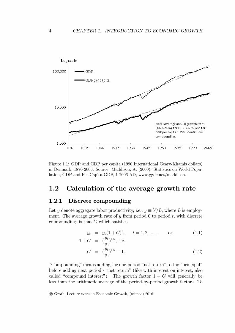
Figure 1.1 displays the time path of annual GDP and GDP per capita in
Denmark 1870-2006 along with regression lines estimated by OLS (logarith-
mic scale on the vertical axis). Figure 1.2 displays the time path of GDP per
capita in UK, USA, and Japan 1870-2006. In both figures the average annual
growth rates are reported. In spite of being based on exactly the same data
as Table 1.1, the numbers are slightly different. Indeed, the numbers in the
figures are slightly lower than those in the table. The reason is that discrete
compounding is used in Table 1.1 while continuous compounding is used in
the two figures. These two alternative methods of calculation are explained
in the next section.
c° Groth, Lecture notes in Economic Growth, (mimeo) 2016.
4 CHAPTER 1. INTRODUCTION TO ECONOMIC GROWTH
Figure 1.1: GDP and GDP per capita (1990 International Geary-Khamis dollars)
in Denmark, 1870-2006. Source: Maddison, A. (2009). Statistics on World Popu-
lation, GDP and Per Capita GDP, 1-2006 AD, www.ggdc.net/maddison.
1.2 Calculation of the average growth rate
1.2.1 Discrete compounding
Let denote aggregate labor productivity, i.e., ≡ where is employ-
ment. The average growth rate of from period 0 to period with discrete
compounding, is that which satisfies
= 0(1 +) = 1 2 , or (1.1)
1 + = (
0)1 i.e.,
= (
0)1 − 1 (1.2)
“Compounding” means adding the one-period “net return” to the “principal”
before adding next period’s “net return” (like with interest on interest, also
called “compound interest”). The growth factor 1 + will generally be
less than the arithmetic average of the period-by-period growth factors. To
c° Groth, Lecture notes in Economic Growth, (mimeo) 2016.

1.2. Calculation of the average growth rate 5
Figure 1.2: GDP per capita (1990 International Geary-Khamis dollars) in UK,
USA and Japan, 1870-2006. Source: Maddison, A. (2009). Statistics on World
Population, GDP and Per Capita GDP, 1-2006 AD, www.ggdc.net/maddison.
underline this difference, 1 + is sometimes called the “compound average
growth factor” or the “geometric average growth factor” and itself then
called the “compound average growth rate” or the “geometric average growth
rate”
Using a pocket calculator, the following steps in the calculation of may
be convenient. Take logs on both sides of (1.1) to get
ln
0= ln(1 +) ⇒
ln(1 +) =ln
0
⇒ (1.3)
= antilog(ln
0
)− 1. (1.4)
Note that in the formulas (1.2) and (1.4) equals the number of periods
minus 1.
c° Groth, Lecture notes in Economic Growth, (mimeo) 2016.

6 CHAPTER 1. INTRODUCTION TO ECONOMIC GROWTH
1.2.2 Continuous compounding
The average growth rate of , with continuous compounding, is that which
satisfies
= 0 (1.5)
where denotes the Euler number, i.e., the base of the natural logarithm.2
Solving for gives
=ln
0
=ln − ln 0
(1.6)
The first formula in (1.6) is convenient for calculation with a pocket calcula-
tor, whereas the second formula is perhaps closer to intuition. Another name
for is the “exponential average growth rate”.
Again, for discrete time data the in the formula equals the number of
periods minus 1.
Comparing with (1.3) we see that = ln(1 +) for 6= 0 Yet, bya first-order Taylor approximation of ln(1 +) about = 0 we have
= ln(1 +) ≈ for “small”. (1.7)
For a given data set the calculated from (1.2) will be slightly above the
calculated from (1.6), cf. the mentioned difference between the growth rates
in Table 1.1 and those in Figure 1.1 and Figure 1.2. The reason is that a given
growth force is more powerful when compounding is continuous rather than
discrete. Anyway, the difference between and is usually unimportant.
If for example refers to the annual GDP growth rate, it will be a small
number, and the difference between and immaterial. For example, to
= 0040 corresponds ≈ 0039 Even if = 010, the corresponding is
00953. But if stands for the inflation rate and there is high inflation, the
difference between and will be substantial. During hyperinflation the
monthly inflation rate may be, say, = 100%, but the corresponding will
be only 69%.
Which method, discrete or continuous compounding, is preferable? To
some extent it is a matter of taste or convenience. In period analysis discrete
compounding is most common and in continuous time analysis continuous
compounding is most common.
For calculation with a pocket calculator the continuous compounding for-
mula, (1.6), is slightly easier to use than the discrete compounding formulas,
whether (1.2) or (1.4).
2Unless otherwise specified, whenever we write ln or log the natural logarithm is
understood.
c° Groth, Lecture notes in Economic Growth, (mimeo) 2016.
1.3. Some stylized facts of economic growth 7
To avoid too much sensitiveness to the initial and terminal observations,
which may involve measurement error or depend on the state of the business
cycle, one can use an OLS approach to the trend coefficient, in the following
regression:
ln = + +
This is in fact what is done in Fig. 1.1.
1.2.3 Doubling time
How long time does it take for to double if the growth rate with discrete
compounding is ? Knowing we rewrite the formula (1.3):
=ln
0
ln(1 +)=
ln 2
ln(1 +)≈ 06931
ln(1 +)
With = 00187 cf. Table 1.1, we find
≈ 374 years,meaning that productivity doubles every 374 years.
How long time does it take for to double if the growth rate with con-
tinuous compounding is ? The answer is based on rewriting the formula
(1.6):
=ln
0
=ln 2
≈ 06931
Maintaining the value 00187 also for we find
≈ 0693100187
≈ 371 years.
Again, with a pocket calculator the continuous compounding formula is
slightly easier to use. With a lower say = 001 we find doubling time
equal to 691 years. With = 007 (think of China since the early 1980’s),
doubling time is about 10 years! Owing to the compounding, exponential
growth is extremely powerful.
1.3 Some stylized facts of economic growth
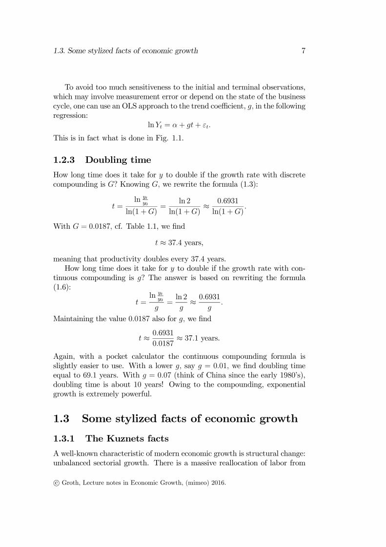
1.3.1 The Kuznets facts
A well-known characteristic of modern economic growth is structural change:
unbalanced sectorial growth. There is a massive reallocation of labor from
c° Groth, Lecture notes in Economic Growth, (mimeo) 2016.

8 CHAPTER 1. INTRODUCTION TO ECONOMIC GROWTH
Figure 1.3: The Kuznets facts. Source: Kongsamut et al., Beyond Balanced
Growth, Review of Economic Studies, vol. 68, Oct. 2001, 869-82.
agriculture into industry (manufacturing, construction, and mining) and fur-
ther into services (including transport and communication). The shares of
total consumption expenditure going to these three sectors have moved sim-
ilarly. Differences in the demand elasticities with respect to income seem the
main explanation. These observations are often referred to as the Kuznets
facts (after Simon Kuznets, 1901-85, see, e.g., Kuznets 1957).
The two graphs in Figure 1.3 illustrate the Kuznets facts.
c° Groth, Lecture notes in Economic Growth, (mimeo) 2016.

1.3. Some stylized facts of economic growth 9
1.3.2 Kaldor’s stylized facts
Surprisingly, in spite of the Kuznets facts, the evolution at the aggregate level
in developed countries is by many economists seen as roughly described by
what is called Kaldor’s “stylized facts” (after the Hungarian-British econo-
mist Nicholas Kaldor, 1908-1986, see, e.g., Kaldor 1957, 1961)3:
1. Real output per man-hour grows at a more or less constant rate
over fairly long periods of time. (Of course, there are short-run fluctuations
superposed around this trend.)
2. The stock of physical capital per man-hour grows at a more or less
constant rate over fairly long periods of time.
3. The ratio of output to capital shows no systematic trend.
4. The rate of return to capital shows no systematic trend.
5. The income shares of labor and capital (in the national account-
ing sense, i.e., including land and other natural resources), respectively, are
nearly constant.
6. The growth rate of output per man-hour differs substantially across
countries.
These claimed regularities do certainly not fit all developed countries
equally well. Although Solow’s growth model (Solow, 1956) can be seen as the
first successful attempt at building a model consistent with Kaldor’s “stylized
facts”, Solow once remarked about them: “There is no doubt that they are
stylized, though it is possible to question whether they are facts” (Solow,
1970). Yet, for instance the study by Attfield and Temple (2010) of US and
UK data since the Second World War concludes with support for Kaldor’s
“facts”. Recently, several empiricists4 have questioned “fact” 5, however,
referring to the inadequacy of the methods which standard national income
accounting applies to separate the income of entrepreneurs, sole proprietors,
and unincorporated businesses into labor and capital income. It is claimed
that these methods obscure a tendency in recent decades of the labor income
share to fall.
The sixth Kaldor fact is, of course, generally accepted as a well docu-
mented observation (a nice summary is contained in Pritchett, 1997).
Kaldor also proposed hypotheses about the links between growth in the
different sectors (see, e.g., Kaldor 1967):
a. Productivity growth in the manufacturing and construction sec-
tors is enhanced by output growth in these sectors (this is also known as
Verdoorn’s Law). Increasing returns to scale and learning by doing are the
main factors behind this.
3Kaldor presented his six regularities as “a stylised view of the facts”.4E.g., Gollin (2002), Elsby et al. (2013), and Karabarbounis and Neiman (2014).
c° Groth, Lecture notes in Economic Growth, (mimeo) 2016.

10 CHAPTER 1. INTRODUCTION TO ECONOMIC GROWTH
b. Productivity growth in agriculture and services is enhanced by out-
put growth in the manufacturing and construction sectors.
Kongsamut et al. (2001) and Foellmi and Zweimüller (2008) offer theoret-
ical explanations of why the Kuznets facts and the Kaldor facts can coexist.
1.4 Concepts of income convergence
The two most popular across-country income convergence concepts are “
convergence” and “ convergence”.
1.4.1 convergence vs. convergence
Definition 1 We say that convergence occurs for a given selection of coun-
tries if there is a tendency for the poor (those with low income per capita or
low output per worker) to subsequently grow faster than the rich.
By “grow faster” is meant that the growth rate of per capita income (or
per worker output) is systematically higher.
In many contexts, a more appropriate convergence concept is the follow-
ing:
Definition 2 We say that convergence, with respect to a given measure of
dispersion, occurs for a given collection of countries if this measure of disper-
sion, applied to income per capita or output per worker across the countries,
declines systematically over time. On the other hand, divergence occurs, if
the dispersion increases systematically over time.
The reason that convergence must be considered the more appropri-
ate concept is the following. In the end, it is the question of increasing
or decreasing dispersion across countries that we are interested in. From a
superficial point of view one might think that convergence implies decreas-
ing dispersion and vice versa, so that convergence and convergence are
more or less equivalent concepts. But since the world is not deterministic,
but stochastic, this is not true. Indeed, convergence is only a necessary,
not a sufficient condition for convergence. This is because over time some
reshuffling among the countries is always taking place, and this implies that
there will always be some extreme countries (those initially far away from
the mean) that move closer to the mean, thus creating a negative correla-
tion between initial level and subsequent growth, in spite of equally many
c° Groth, Lecture notes in Economic Growth, (mimeo) 2016.

1.4. Concepts of income convergence 11
countries moving from a middle position toward one of the extremes.5 In
this way convergence may be observed at the same time as there is no
convergence; the mere presence of random measurement errors implies a bias
in this direction because a growth rate depends negatively on the initial mea-
surement and positively on the later measurement. In fact, convergence
may be consistent with divergence (for a formal proof of this claim, see
Barro and Sala-i-Martin, 2004, pp. 50-51 and 462 ff.; see also Valdés, 1999,
p. 49-50, and Romer, 2001, p. 32-34).
Hence, it is wrong to conclude from convergence (poor countries tend
to grow faster than rich ones) to convergence (reduced dispersion of per
capita income) without any further investigation. The mistake is called “re-
gression towards the mean” or “Galton’s fallacy”. Francis Galton was an
anthropologist (and a cousin of Darwin), who in the late nineteenth century
observed that tall fathers tended to have not as tall sons and small fathers
tended to have taller sons. From this he falsely concluded that there was
a tendency to averaging out of the differences in height in the population.
Indeed, being a true aristocrat, Galton found this tendency pitiable. But
since his conclusion was mistaken, he did not really have to worry.
Since convergence comes closer to what we are ultimately looking for,
from now, when we speak of just “income convergence”, convergence is
understood.
In the above definitions of convergence and convergence, respectively,
we were vague as to what kind of selection of countries is considered. In
principle we would like it to be a representative sample of the “population”
of countries that we are interested in. The population could be all countries
in the world. Or it could be the countries that a century ago had obtained a
certain level of development.
One should be aware that historical GDP data are constructed retrospec-
tively. Long time series data have only been constructed for those countries
that became relatively rich during the after-WWII period. Thus, if we as our
sample select the countries for which long data series exist, what is known as
selection bias is involved which generates a spurious convergence. A country
which was poor a century ago will only appear in the sample if it grew rapidly
over the next 100 years. A country which was relatively rich a century ago
will appear in the sample unconditionally. This selection bias problem was
5As an intuitive analogy, think of the ordinal rankings of the sports teams in a league.
The dispersion of rankings is constant by definition. Yet, no doubt there will allways be
some tendency for weak teams to rebound toward the mean and of champions to revert
to mediocrity. (This example is taken from the first edition of Barro and Sala-i-Martin,
Economic Growth, 1995; I do not know why, but the example was deleted in the second
edition from 2004.)
c° Groth, Lecture notes in Economic Growth, (mimeo) 2016.
12 CHAPTER 1. INTRODUCTION TO ECONOMIC GROWTH
pointed out by DeLong (1988) in a criticism of widespread false interpreta-
tions of Maddison’s long data series (Maddison 1982).
1.4.2 Measures of dispersion
Our next problem is: what measure of dispersion is to be used as a useful
descriptive statistics for convergence? Here there are different possibilities.
To be precise about this we need some notation. Let
≡
and
≡
where = real GDP, = employment, and = population. If the focus
is on living standards, is the relevant variable.6 But if the focus is on
(labor) productivity, it is that is relevant. Since most growth models
focus on rather than let os take as our example.
One might think that the standard deviation of could be a relevant
measure of dispersion when discussing whether convergence is present or
not. The standard deviation of across countries in a given year is
≡vuut1
X=1
( − )2 (1.8)
where
≡P
(1.9)
i.e., is the average output per worker. However, if this measure were used,
it would be hard to find any group of countries for which there is income
convergence. This is because tends to grow over time for most countries,
and then there is an inherent tendency for the variance also to grow; hence
also the square root of the variance, tends to grow. Indeed, suppose that
for all countries, is doubled from time 1 to time 2 Then, automatically,
is also doubled. But hardly anyone would interpret this as an increase in
the income inequality across the countries.
Hence, it is more adequate to look at the standard deviation of relative
income levels:
≡s1
X
(
− 1)2 (1.10)
6Or perhaps better, where ≡ ≡ − − Here, denotes net
interest payments on foreign debt and denotes net labor income of foreign workers in
the country.
c° Groth, Lecture notes in Economic Growth, (mimeo) 2016.

1.4. Concepts of income convergence 13
This measure is the same as what is called the coefficient of variation,
usually defined as
≡
(1.11)
that is, the standard deviation of standardized by the mean. That the two
measures are identical can be seen in this way:
≡
q1
P( − )2
=
s1
X
( −
)2 =
s1
X
(
− 1)2 ≡
The point is that the coefficient of variation is “scale free”, which the standard
deviation itself is not.
Instead of the coefficient of variation, another scale free measure is often
used, namely the standard deviation of ln , i.e.,
ln ≡s1
X
(ln − ln ∗)2 (1.12)
where
ln ∗ ≡P
ln
(1.13)
Note that ∗ is the geometric average, i.e., ∗ ≡ √12 · · · Now, by a
first-order Taylor approximation of ln around = , we have
ln ≈ ln + 1( − )
Hence, as a very rough approximation we have ln ≈ = though
this approximation can be quite poor (cf. Dalgaard and Vastrup, 2001).
It may be possible, however, to defend the use of ln in its own right to
the extent that tends to be approximately lognormally distributed across
countries.
Yet another possible measure of income dispersion across countries is the
Gini index (see for example Cowell, 1995).
1.4.3 Weighting by size of population
Another important issue is whether the applied dispersion measure is based
on a weighting of the countries by size of population. For the world as a
whole, when no weighting by size of population is used, then there is a slight
tendency to income divergence according to the ln criterion (Acemoglu,
c° Groth, Lecture notes in Economic Growth, (mimeo) 2016.

14 CHAPTER 1. INTRODUCTION TO ECONOMIC GROWTH
2009, p. 4), where is per capita income (≡ ). As seen by Fig. 4 below,
this tendency is not so clear according to the criterion. Anyway, when
there is weighting by size of population, then in the last twenty years there
has been a tendency to income convergence at the global level (Sala-i-Martin
2006; Acemoglu, 2009, p. 6). With weighting by size of population (1.12) is
modified to
ln ≡sX
(ln − ln ∗)2
where
=
and ln ∗ ≡
X
ln
1.4.4 Unconditional vs. conditional convergence
Yet another distinction in the study of income convergence is that between
unconditional (or absolute) and conditional convergence. We say that a
large heterogeneous group of countries (say the countries in the world) show
unconditional income convergence if income convergence occurs for the whole
group without conditioning on specific characteristics of the countries. If
income convergence occurs only for a subgroup of the countries, namely those
countries that in advance share the same “structural characteristics”, then
we say there is conditional income convergence. As noted earlier, when we
speak of just income “convergence”, income “ convergence” is understood.
If in a given context there might be doubt, one should of course be explicit
and speak of unconditional or conditional convergence. Similarly, if the
focus for some reason is on convergence, we should distinguish between
unconditional and conditional convergence.
What the precise meaning of “structural characteristics” is, will depend
on what model of the countries the researcher has in mind. According to
the Solow model, a set of relevant “structural characteristics” are: the aggre-
gate production function, the initial level of technology, the rate of technical
progress, the capital depreciation rate, the saving rate, and the population
growth rate. But the Solow model, as well as its extension with human cap-
ital (Mankiw et al., 1992), is a model of a closed economy with exogenous
technical progress. The model deals with “within-country” convergence in
the sense that the model predicts that a closed economy being initially be-
low or above its steady state path, will over time converge towards its steady
state path. It is far from obvious that this kind of model is a good model
of cross-country convergence in a globalized world where capital mobility
and to some extent also labor mobility are important and some countries are
c° Groth, Lecture notes in Economic Growth, (mimeo) 2016.

1.4. Concepts of income convergence 15
0
3000
6000
9000
12000
15000
18000
21000
1950 1960 1970 1980 1990 2000
Dispersion of GDP per capita
Dispersion of GDP per worker
Dispersion
Year
Remarks: Germany is not included in GDP per worker. GDP per worker is missing for Sweden and Greece in 1950, and for Portugal in 1998. The EU comprises Belgium, Denmark, Finland, France, Greece, Holland, Ireland, Italy, Luxembourg, Portugal, Spain, Sweden, Germany, the UK and Austria. Source: Pwt6, OECD Economic Outlook No. 65 1999 via Eco Win and World Bank Global Development Network Growth Database.
Figure 1.4: Standard deviation of GDP per capita and per worker across 12 EU
countries, 1950-1998.
pushing the technological frontier further out, while others try to imitate and
catch up.
1.4.5 A bird’s-eye view of the data
In the following no serious econometrics is attempted. We use the term
“trend” in an admittedly loose sense.
Figure 1.4 shows the time profile for the standard deviation of itself for
12 EU countries, whereas Figure 1.5 and Figure 1.6 show the time profile
of the standard deviation of log and the time profile of the coefficient of
variation, respectively. Comparing the upward trend in Figure 1.4 with the
downward trend in the two other figures, we have an illustration of the fact
that the movement of the standard deviation of itself does not capture
income convergence. To put it another way: although there seems to be
conditional income convergence with respect to the two scale-free measures,
Figure 1.4 shows that this tendency to convergence is not so strong as to
produce a narrowing of the absolute distance between the EU countries.7
7Unfortunately, sometimes misleading graphs or texts to graphs about across-country
c° Groth, Lecture notes in Economic Growth, (mimeo) 2016.

16 CHAPTER 1. INTRODUCTION TO ECONOMIC GROWTH
0
0,04
0,08
0,12
0,16
0,2
0,24
0,28
0,32
0,36
0,4
1950 1960 1970 1980 1990 2000
Dispersion
Dispersion of the log of GDP per capita
Dispersion of the log of GDP per worker
Year
Remarks: Germany is not included in GDP per worker. GDP per worker is missing for Sweden and Greece in 1950, and for Portugal in 1998. The EU comprises Belgium, Denmark, Finland, France, Greece, Holland, Ireland, Italy, Luxembourg, Portugal, Spain, Sweden, Germany, the UK and Austria. Source: Pwt6, OECD Economic Outlook No. 65 1999 via Eco Win and World Bank Global Development Network Growth Database.
Figure 1.5: Standard deviation of the log of GDP per capita and per worker across
12 EU countries, 1950-1998.
c° Groth, Lecture notes in Economic Growth, (mimeo) 2016.

1.4. Concepts of income convergence 17
0
0,1
0,2
0,3
0,4
0,5
0,6
0,7
0,8
0,9
1950 1960 1970 1980 1990 2000
Coefficient of variation
Coefficient of variation for GDP per capita
Coefficient of variation for GDP per worker
Year
Remarks: Germany is not included in GDP per worker. GDP per worker is missing for Sweden and Greece in 1950, and for Portugal in 1998. The EU comprises Belgium, Denmark, Finland, France, Greece, Holland, Ireland, Italy, Luxembourg, Portugal, Spain, Sweden, Germany, the UK and Austria. Source: Pwt6, OECD Economic Outlook No. 65 1999 via Eco Win and World Bank Global Development Network Growth Database.
Figure 1.6: Coefficient of variation of GDP per capita and GDP per worker across
12 EU countries, 1950-1998.
Figure 1.7 shows the time path of the coefficient of variation across 121
countries in the world, 22 OECD countries and 12 EU countries, respectively.
We see the lack of unconditional income convergence, but the presence of con-
ditional income convergence. One should not over-interpret the observation
of convergence for the 22 OECD countries over the period 1950-1990. It is
likely that this observation suffer from the selection bias problem mentioned
in Section 1.4.1. A country that was poor in 1950 will typically have become
a member of OECD only if it grew relatively fast afterwards.
1.4.6 Other convergence concepts
Of course, just considering the time profile of the first and second moments
of a distribution may sometimes be a poor characterization of the evolution
of the distribution. For example, there are signs that the distribution has
polarized into twin peaks of rich and poor countries (Quah, 1996a; Jones,
income convergence are published. In the collection of exercises, Chapter 1, you are asked
to discuss some examples of this.
c° Groth, Lecture notes in Economic Growth, (mimeo) 2016.

18 CHAPTER 1. INTRODUCTION TO ECONOMIC GROWTH
0
0,2
0,4
0,6
0,8
1
1,2
1950 1953 1956 1959 1962 1965 1968 1971 1974 1977 1980 1983 1986 1989 1992 1995
Coefficient of variation
22 OECD countries (1950-90)
EU-12 (1960-95)
The world (1960-88)
Remarks: 'The world' comprises 121 countries (not weighed by size) where complete time series for GDP per capita exist. The OECD countries exclude South Korea, Hungary, Poland, Iceland, Czech Rep., Luxembourg and Mexico. EU-12 comprises: Benelux, Germany, France, Italy, Denmark, Ireland, UK, Spain, Portugal og Greece. Source: Penn World Table 5.6 and OECD Economic Outlook, Statistics on Microcomputer Disc, December 1998.
Coefficient of variation
Figure 1.7: Coefficient of variation of income per capita across different sets of
countries.
1997). Related to this observation is the notion of club convergence. If in-
come convergence occurs only among a subgroup of the countries that to
some extent share the same initial conditions, then we say there is club-
convergence. This concept is relevant in a setting where there are multiple
steady states toward which countries can converge. At least at the theoret-
ical level multiple steady states can easily arise in overlapping generations
models. Then the initial condition for a given country matters for which of
these steady states this country is heading to. Similarly, we may say that
conditional club-convergence is present, if income convergence occurs only
for a subgroup of the countries, namely countries sharing similar structural
characteristics (this may to some extent be true for the OECD countries)
and, within an interval, similar initial conditions.
Instead of focusing on income convergence, one could study TFP conver-
gence at aggregate or industry level.8 Sometimes the less demanding concept
of growth rate convergence is the focus.
The above considerations are only of a very elementary nature and are
only about descriptive statistics. The reader is referred to the large existing
literature on concepts and econometric methods of relevance for character-
8See, for instance, Bernard and Jones 1996a and 1996b.
c° Groth, Lecture notes in Economic Growth, (mimeo) 2016.

1.5. Literature 19
izing the evolution of world income distribution (see Quah, 1996b, 1996c,
1997, and for a survey, see Islam 2003).
1.5 Literature
Acemoglu, D., 2009, Introduction to Modern Economic Growth, Princeton
University Press: Oxford.
Acemoglu, D., and V. Guerrieri, 2008, Capital deepening and nonbalanced
economic growth, J. Political Economy, vol. 116 (3), 467- .
Attfield, C., and J.R.W. Temple, 2010, Balanced growth and the great
ratios: New evidence for the US and UK, Journal of Macroeconomics,
vol. 32, 937-956.
Barro, R. J., and X. Sala-i-Martin, 1995, Economic Growth, MIT Press,
New York. Second edition, 2004.
Bernard, A.B., and C.I. Jones, 1996a, ..., Economic Journal.
- , 1996b, Comparing Apples to Oranges: Productivity Convergence and
Measurement Across Industries and Countries, American Economic
Review, vol. 86 (5), 1216-1238.
Cowell, Frank A., 1995, Measuring Inequality. 2. ed., London.
Dalgaard, C.-J., and J. Vastrup, 2001, On the measurement of -convergence,
Economics letters, vol. 70, 283-87.
Dansk økonomi. Efterår 2001, (Det økonomiske Råds formandskab) Kbh.
2001.
Deininger, K., and L. Squire, 1996, A new data set measuring income in-
equality, The World Bank Economic Review, 10, 3.
Delong, B., 1988, ... American Economic Review.
Foellmi, R., and J. Zweimüller, 2008, ..., JME, 55, 1317-1328.
Handbook of Economic Growth, vol. 1A and 1B, ed. by S. N. Durlauf and
P. Aghion, Amsterdam 2005.
Handbook of Income Distribution, vol. 1, ed. by A.B. Atkinson and F.
Bourguignon, Amsterdam 2000.
c° Groth, Lecture notes in Economic Growth, (mimeo) 2016.
20 CHAPTER 1. INTRODUCTION TO ECONOMIC GROWTH
Islam, N., 2003, What have we learnt from the convergence debate? Journal
of Economic Surveys 17, 3, 309-62.
Kaldor, N., 1957, A model of economic growth, The Economic Journal, vol.
67, pp. 591-624.
- , 1961, “Capital Accumulation and Economic Growth”. In: F. Lutz, ed.,
Theory of Capital, London: MacMillan.
- , 1967, Strategic Factors in Economic Development, New York State School
of Industrial and Labor Relations, Cornell University.
Kongsamut, P., S. Rebelo, and D. Xie, 2001, Beyond Balanced Growth,
Review of Economic Studies, vol. 68, 869-882.
Kuznets, S., 1957, Quantitative aspects of economic growth of nations: II,
Economic Development and Cultural Change, Supplement to vol. 5,
3-111.
Maddison, A., 1982,
Maddison, A., Contours ...., Cambridge University Press.
Mankiw, N.G., D. Romer, and D.N. Weil, 1992,
Pritchett, L., 1997, Divergence — big time, Journal of Economic Perspec-
tives, vol. 11, no. 3.
Quah, D., 1996a, Twin peaks ..., Economic Journal, vol. 106, 1045-1055.
-, 1996b, Empirics for growth and convergence, European Economic Review,
vol. 40 (6).
-, 1996c, Convergence empirics ..., J. of Ec. Growth, vol. 1 (1).
-, 1997, Searching for prosperity: A comment, Carnegie-Rochester Confer-
ende Series on Public Policy, vol. 55, 305-319.
Romer, D., 2012, Advanced Macroeconomics, 4th ed., McGraw-Hill: New
York.
Sala-i-Martin, X., 2006, The World Distribution of Income, Quarterly Jour-
nal of Economics 121, No. 2.
Sen, A., ...
c° Groth, Lecture notes in Economic Growth, (mimeo) 2016.

1.5. Literature 21
Solow, R.M., 1970, Growth theory. An exposition, Clarendon Press: Oxford.
Second enlarged edition, 2000.
Valdés, B., 1999, Economic Growth. Theory, Empirics, and Policy, Edward
Elgar.
Onmeasurement problems, see: http://www.worldbank.org/poverty/inequal/methods/index.htm
c° Groth, Lecture notes in Economic Growth, (mimeo) 2016.

22 CHAPTER 1. INTRODUCTION TO ECONOMIC GROWTH
c° Groth, Lecture notes in Economic Growth, (mimeo) 2016.

Chapter 2
Review of technology andfactor shares of income
The aim of this chapter is, first, to introduce the terminology concerningfirms’technology and technological change used in the lectures and exercisesof this course. At a few points I deviate somewhat from definitions in Ace-moglu’s book. Section 1.3 can be used as a formula manual for the case ofCRS.Second, the chapter contains a brief discussion of the notions of a repre-
sentative firm and an aggregate production function. The distinction betweenlong-run versus short-run production functions is also commented on. Thelast sections introduce the concept of elasticity of substitution between cap-ital and labour and its role for the direction of movement over time of theincome shares of capital and labor under perfect competition.Regarding the distinction between discrete and continuous time analysis,
most of the definitions contained in this chapter are applicable to both.
2.1 The production technology
Consider a two-factor production function given by
Y = F (K,L), (2.1)
where Y is output (value added) per time unit, K is capital input per timeunit, and L is labor input per time unit (K ≥ 0, L ≥ 0). We may think of(2.1) as describing the output of a firm, a sector, or the economy as a whole.It is in any case a very simplified description, ignoring the heterogeneity ofoutput, capital, and labor. Yet, for many macroeconomic questions it maybe a useful first approach. Note that in (2.1) not only Y but also K and L
23

24CHAPTER 2. REVIEW OF TECHNOLOGY AND
FACTOR SHARES OF INCOME
represent flows, that is, quantities per unit of time. If the time unit is oneyear, we think of K as measured in machine hours per year. Similarly, wethink of L as measured in labor hours per year. Unless otherwise specified, itis understood that the rate of utilization of the production factors is constantover time and normalized to one for each production factor. As explainedin Chapter 1, we can then use the same symbol, K, for the flow of capitalservices as for the stock of capital. Similarly with L.
2.1.1 A neoclassical production function
By definition, K and L are non-negative. It is generally understood that aproduction function, Y = F (K,L), is continuous and that F (0, 0) = 0 (no in-put, no output). Sometimes, when specific functional forms are used to repre-sent a production function, that function may not be defined at points whereK = 0 or L = 0 or both. In such a case we adopt the convention that the do-main of the function is understood extended to include such boundary pointswhenever it is possible to assign function values to them such that continuityis maintained. For instance the function F (K,L) = αL + βKL/(K + L),where α > 0 and β > 0, is not defined at (K,L) = (0, 0). But by assigningthe function value 0 to the point (0, 0), we maintain both continuity and the“no input, no output”property.We call the production function neoclassical if for all (K,L), with K > 0
and L > 0, the following additional conditions are satisfied:
(a) F (K,L) has continuous first- and second-order partial derivatives sat-isfying:
FK > 0, FL > 0, (2.2)
FKK < 0, FLL < 0. (2.3)
(b) F (K,L) is strictly quasiconcave (i.e., the level curves, also called iso-quants, are strictly convex to the origin).
In words: (a) says that a neoclassical production function has continuoussubstitution possibilities between K and L and the marginal productivitiesare positive, but diminishing in own factor. Thus, for a given number of ma-chines, adding one more unit of labor, adds to output, but less so, the higheris already the labor input. And (b) says that every isoquant, F (K,L) = Y ,has a strictly convex form qualitatively similar to that shown in Figure 2.1.1
1For any fixed Y ≥ 0, the associated isoquant is the level set{(K,L) ∈ R+| F (K,L) = Y
}.
c© Groth, Lecture notes in Economic Growth, (mimeo) 2016.

2.1. The production technology 25
When we speak of for example FL as the marginal productivity of labor, itis because the “pure” partial derivative, ∂Y/∂L = FL, has the denomina-tion of a productivity (output units/yr)/(man-yrs/yr). It is quite common,however, to refer to FL as the marginal product of labor. Then a unit mar-ginal increase in the labor input is understood: ∆Y ≈ (∂Y/∂L)∆L = ∂Y/∂Lwhen ∆L = 1. Similarly, FK can be interpreted as the marginal productiv-ity of capital or as the marginal product of capital. In the latter case it isunderstood that ∆K = 1, so that ∆Y ≈ (∂Y/∂K)∆K = ∂Y/∂K.
The definition of a neoclassical production function can be extended tothe case of n inputs. Let the input quantities be X1, X2, . . . , Xn and considera production function Y = F (X1, X2, . . . , Xn). Then F is called neoclassical ifall the marginal productivities are positive, but diminishing, and F is strictlyquasiconcave (i.e., the upper contour sets are strictly convex, cf. AppendixA).Returning to the two-factor case, since F (K,L) presumably depends on
the level of technical knowledge and this level depends on time, t, we mightwant to replace (2.1) by
Yt = F t(Kt, Lt), (2.4)
where the superscript on F indicates that the production function may shiftover time, due to changes in technology. We then say that F t(·) is a neoclas-sical production function if it satisfies the conditions (a) and (b) for all pairs(Kt, Lt). Technological progress can then be said to occur when, for Kt andLt held constant, output increases with t.For convenience, to begin with we skip the explicit reference to time and
level of technology.
The marginal rate of substitution Given a neoclassical productionfunction F, we consider the isoquant defined by F (K,L) = Y , where Yis a positive constant. The marginal rate of substitution, MRSKL, of K forL at the point (K,L) is defined as the absolute slope of the isoquant at thatpoint, cf. Figure 2.1. The equation F (K,L) = Y defines K as an implicitfunction of L. By implicit differentiation we find FK(K,L)dK/dL +FL(K,L)= 0, from which follows
MRSKL ≡ −dK
dL |Y=Y=FL(K,L)
FK(K,L)> 0. (2.5)
That is, MRSKL measures the amount of K that can be saved (approxi-mately) by applying an extra unit of labor. In turn, this equals the ratio
c© Groth, Lecture notes in Economic Growth, (mimeo) 2016.

26CHAPTER 2. REVIEW OF TECHNOLOGY AND
FACTOR SHARES OF INCOME
Figure 2.1: MRSKL as the absolute slope of the isoquant.
of the marginal productivities of labor and capital, respectively.2 Since Fis neoclassical, by definition F is strictly quasi-concave and so the marginalrate of substitution is diminishing as substitution proceeds, i.e., as the laborinput is further increased along a given isoquant. Notice that this featurecharacterizes the marginal rate of substitution for any neoclassical productionfunction, whatever the returns to scale (see below).When we want to draw attention to the dependency of the marginal rate of
substitution on the factor combination considered, we write MRSKL(K,L).Sometimes in the literature, the marginal rate of substitution between twoproduction factors, K and L, is called the technical rate of substitution (orthe technical rate of transformation) in order to distinguish from a consumer’smarginal rate of substitution between two consumption goods.As is well-known from microeconomics, a firm that minimizes production
costs for a given output level and given factor prices, will choose a factor com-bination such that MRSKL equals the ratio of the factor prices. If F (K,L)is homogeneous of degree q, then the marginal rate of substitution dependsonly on the factor proportion and is thus the same at any point on the rayK = (K/L)L. That is, in this case the expansion path is a straight line.
The Inada conditions A continuously differentiable production functionis said to satisfy the Inada conditions3 if
limK→0
FK(K,L) = ∞, limK→∞
FK(K,L) = 0, (2.6)
limL→0
FL(K,L) = ∞, limL→∞
FL(K,L) = 0. (2.7)
2The subscript∣∣Y = Y in (2.5) indicates that we are moving along a given isoquant,
F (K,L) = Y . Expressions like, e.g., FL(K,L) or F2(K,L) mean the partial derivative ofF w.r.t. the second argument, evaluated at the point (K,L).
3After the Japanese economist Ken-Ichi Inada, 1925-2002.
c© Groth, Lecture notes in Economic Growth, (mimeo) 2016.

2.1. The production technology 27
In this case, the marginal productivity of either production factor has noupper bound when the input of the factor becomes infinitely small. And themarginal productivity is gradually vanishing when the input of the factorincreases without bound. Actually, (2.6) and (2.7) express four conditions,which it is preferable to consider separately and label one by one. In (2.6) wehave two Inada conditions for MPK (the marginal productivity of capital),the first being a lower, the second an upper Inada condition for MPK. Andin (2.7) we have two Inada conditions for MPL (the marginal productivityof labor), the first being a lower, the second an upper Inada condition forMPL. In the literature, when a sentence like “the Inada conditions areassumed”appears, it is sometimes not made clear which, and how many, ofthe four are meant. Unless it is evident from the context, it is better to beexplicit about what is meant.The definition of a neoclassical production function we gave above is quite
common in macroeconomic journal articles and convenient because of itsflexibility. There are textbooks that define a neoclassical production functionmore narrowly by including the Inada conditions as a requirement for callingthe production function neoclassical. In contrast, in this course, when in agiven context we need one or another Inada condition, we state it explicitlyas an additional assumption.
2.1.2 Returns to scale
If all the inputs are multiplied by some factor, is output then multiplied bythe same factor? There may be different answers to this question, dependingon circumstances. We consider a production function F (K,L) where K > 0and L > 0. Then F is said to have constant returns to scale (CRS for short)if it is homogeneous of degree one, i.e., if for all (K,L) and all λ > 0,
F (λK, λL) = λF (K,L).
As all inputs are scaled up or down by some factor > 1, output is scaled upor down by the same factor.4 The assumption of CRS is often defended bythe replication argument. Before discussing this argument, lets us define thetwo alternative “pure”cases.The production function F (K,L) is said to have increasing returns to
scale (IRS for short) if, for all (K,L) and all λ > 1,
F (λK, λL) > λF (K,L).
4In their definition of a neoclassical production function some textbooks add constantreturns to scale as a requirement besides (a) and (b). This course follows the alternativeterminology where, if in a given context an assumption of constant returns to scale isneeded, this is stated as an additional assumption.
c© Groth, Lecture notes in Economic Growth, (mimeo) 2016.

28CHAPTER 2. REVIEW OF TECHNOLOGY AND
FACTOR SHARES OF INCOME
That is, IRS is present if, when all inputs are scaled up by some factor >1, output is scaled up by more than this factor. The existence of gains byspecialization and division of labor, synergy effects, etc. sometimes speak insupport of this assumption, at least up to a certain level of production. Theassumption is also called the economies of scale assumption.Another possibility is decreasing returns to scale (DRS). This is said to
occur when for all (K,L) and all λ > 1,
F (λK, λL) < λF (K,L).
That is, DRS is present if, when all inputs are scaled up by some factor,output is scaled up by less than this factor. This assumption is also calledthe diseconomies of scale assumption. The underlying hypothesis may bethat control and coordination problems confine the expansion of size. Or,considering the “replication argument”below, DRS may simply reflect thatbehind the scene there is an additional production factor, for example landor a irreplaceable quality of management, which is tacitly held fixed, whenthe factors of production are varied.
EXAMPLE 1 The production function
Y = AKαLβ, A > 0, 0 < α < 1, 0 < β < 1, (2.8)
where A, α, and β are given parameters, is called a Cobb-Douglas productionfunction. The parameter A depends on the choice of measurement units;for a given such choice it reflects “effi ciency”, also called the “total factorproductivity”. As an exercise the reader may verify that (2.8) satisfies (a) and(b) above and is therefore a neoclassical production function. The functionis homogeneous of degree α + β. If α + β = 1, there are CRS. If α + β < 1,there are DRS, and if α + β > 1, there are IRS. Note that α and β mustbe less than 1 in order not to violate the diminishing marginal productivitycondition. �EXAMPLE 2 The production function
Y = min(AK,BL), A > 0, B > 0, (2.9)
where A and B are given parameters, is called a Leontief production functionor a fixed-coeffi cients production function; A and B are called the technicalcoeffi cients. The function is not neoclassical, since the conditions (a) and (b)are not satisfied. Indeed, with this production function the production fac-tors are not substitutable at all. This case is also known as the case of perfectcomplementarity between the production factors. The interpretation is that
c© Groth, Lecture notes in Economic Growth, (mimeo) 2016.

2.1. The production technology 29
already installed production equipment requires a fixed number of workers tooperate it. The inverse of the parameters A and B indicate the required cap-ital input per unit of output and the required labor input per unit of output,respectively. Extended to many inputs, this type of production function isoften used in multi-sector input-output models (also called Leontief models).In aggregate analysis neoclassical production functions, allowing substitutionbetween capital and labor, are more popular than Leontief functions. Butsometimes the latter are preferred, in particular in short-run analysis withfocus on the use of already installed equipment where the substitution pos-sibilities are limited.5 As (2.9) reads, the function has CRS. A generalizedform of the Leontief function is Y = min(AKγ, BLγ), where γ > 0. Whenγ < 1, there are DRS, and when γ > 1, there are IRS. �
The replication argument The assumption of CRS is widely used inmacroeconomics. The model builder may appeal to the replication argument.This is the argument saying that by doubling all the inputs, we should alwaysbe able to double the output, since we are just “replicating”what we arealready doing. Suppose we want to double the production of cars. We maythen build another factory identical to the one we already have, man it withidentical workers and deploy the same material inputs. Then it is reasonableto assume output is doubled.In this context it is important that the CRS assumption is about tech-
nology in the sense of functions linking outputs to inputs. Limits to theavailability of input resources is an entirely different matter. The fact thatfor example managerial talent may be in limited supply does not preclude thethought experiment that if a firm could double all its inputs, including thenumber of talented managers, then the output level could also be doubled.The replication argument presupposes, first, that all the relevant inputs
are explicit as arguments in the production function; second, that these arechanged equiproportionately. This, however, exhibits the weakness of thereplication argument as a defence for assuming CRS of our present productionfunction, F (·). One could easily make the case that besides capital and labor,also land is a necessary input and should appear as a separate argument.6
If an industrial firm decides to duplicate what it has been doing, it needs apiece of land to build another plant like the first. Then, on the basis of thereplication argument we should in fact expect DRS w.r.t. capital and laboralone. In manufacturing and services, empirically, this and other possible
5Cf. Section 2.4.6We think of “capital” as producible means of production, whereas “land” refers to
non-producible natural resources, including for example building sites.
c© Groth, Lecture notes in Economic Growth, (mimeo) 2016.

30CHAPTER 2. REVIEW OF TECHNOLOGY AND
FACTOR SHARES OF INCOME
sources for departure from CRS may be minor and so many macroeconomistsfeel comfortable enough with assuming CRS w.r.t. K and L alone, at leastas a first approximation. This approximation is, however, less applicable topoor countries, where natural resources may be a quantitatively importantproduction factor.There is a further problem with the replication argument. Strictly speak-
ing, the CRS claim is that by changing all the inputs equiproportionatelyby any positive factor, λ, which does not have to be an integer, the firmshould be able to get output changed by the same factor. Hence, the replica-tion argument requires that indivisibilities are negligible, which is certainlynot always the case. In fact, the replication argument is more an argumentagainst DRS than for CRS in particular. The argument does not rule outIRS due to synergy effects as size is increased.Sometimes the replication line of reasoning is given a more subtle form.
This builds on a useful local measure of returns to scale, named the elasticityof scale.
The elasticity of scale* To allow for indivisibilities and mixed cases (forexample IRS at low levels of production and CRS or DRS at higher levels),we need a local measure of returns to scale. One defines the elasticity ofscale, η(K,L), of F at the point (K,L), where F (K,L) > 0, as
η(K,L) =λ
F (K,L)
dF (λK, λL)
dλ≈ ∆F (λK, λL)/F (K,L)
∆λ/λ, evaluated at λ = 1.
(2.10)So the elasticity of scale at a point (K,L) indicates the (approximate) per-centage increase in output when both inputs are increased by 1 percent. Wesay that
if η(K,L)
> 1, then there are locally IRS,= 1, then there are locally CRS,< 1, then there are locally DRS.
(2.11)
The production function may have the same elasticity of scale everywhere.This is the case if and only if the production function is homogeneous. If Fis homogeneous of degree h, then η(K,L) = h and h is called the elasticityof scale parameter.Note that the elasticity of scale at a point (K,L) will always equal the
sum of the partial output elasticities at that point:
η(K,L) =FK(K,L)K
F (K,L)+FL(K,L)L
F (K,L). (2.12)
This follows from the definition in (2.10) by taking into account that
c© Groth, Lecture notes in Economic Growth, (mimeo) 2016.
2.1. The production technology 31
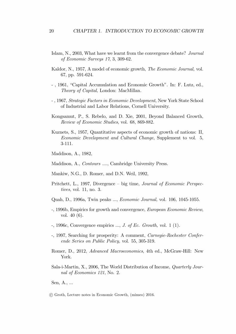
Figure 2.2: Locally CRS at optimal plant size.
dF (λK, λL)
dλ= FK(λK, λL)K + FL(λK, λL)L
= FK(K,L)K + FL(K,L)L, when evaluated at λ = 1.
Figure 2.2 illustrates a popular case from introductory economics, anaverage cost curve which from the perspective of the individual firm (or plant)is U-shaped: at low levels of output there are falling average costs (thus IRS),at higher levels rising average costs (thus DRS).7 Given the input prices, wKand wL, and a specified output level, Y , we know that the cost minimizingfactor combination (K, L) is such that FL(K, L)/FK(K, L) = wL/wK . It isshown in Appendix A that the elasticity of scale at (K, L) will satisfy:
η(K, L) =LAC(Y )
LMC(Y ), (2.13)
where LAC(Y ) is average costs (the minimum unit cost associated withproducing Y ) and LMC(Y ) is marginal costs at the output level Y . TheL in LAC and LMC stands for “long-run”, indicating that both capital andlabor are considered variable production factors within the period considered.At the optimal plant size, Y ∗, there is equality between LAC and LMC,implying a unit elasticity of scale, that is, locally we have CRS. That the long-run average costs are here portrayed as rising for Y > Y ∗, is not essentialfor the argument but may reflect either that coordination diffi culties areinevitable or that some additional production factor, say the building site ofthe plant, is tacitly held fixed.Anyway, we have here a more subtle replication argument for CRS w.r.t.
K and L at the aggregate level. Even though technologies may differ acrossplants, the surviving plants in a competitive market will have the same aver-age costs at the optimal plant size. In the medium and long run, changes in
7By a “firm”is generally meant the company as a whole. A company may have several“manufacturing plants”placed at different locations.
c© Groth, Lecture notes in Economic Growth, (mimeo) 2016.
32CHAPTER 2. REVIEW OF TECHNOLOGY AND
FACTOR SHARES OF INCOME
aggregate output will take place primarily by entry and exit of optimal-sizeplants. Then, with a large number of relatively small plants, each produc-ing at approximately constant unit costs for small output variations, we canwithout substantial error assume constant returns to scale at the aggregatelevel. So the argument goes. Notice, however, that even in this form thereplication argument is not entirely convincing since the question of indivis-ibility remains. The optimal plant size may be large relative to the market− and is in fact so in many industries. Besides, in this case also the perfectcompetition premise breaks down.
2.1.3 Properties of the production function under CRS
The empirical evidence concerning returns to scale is mixed. Notwithstand-ing the theoretical and empirical ambiguities, the assumption of CRS w.r.t.capital and labor has a prominent role in macroeconomics. In many con-texts it is regarded as an acceptable approximation and a convenient simplebackground for studying the question at hand.Expedient inferences of the CRS assumption include:
(i) marginal costs are constant and equal to average costs (so the right-hand side of (2.13) equals unity);
(ii) if production factors are paid according to their marginal productivi-ties, factor payments exactly exhaust total output so that pure profitsare neither positive nor negative (so the right-hand side of (2.12) equalsunity);
(iii) a production function known to exhibit CRS and satisfy property (a)from the definition of a neoclassical production function above, will au-tomatically satisfy also property (b) and consequently be neoclassical;
(iv) a neoclassical two-factor production function with CRS has alwaysFKL > 0, i.e., it exhibits “direct complementarity” between K andL;
(v) a two-factor production function known to have CRS and to be twicecontinuously differentiable with positive marginal productivity of eachfactor everywhere in such a way that all isoquants are strictly convex tothe origin, must have diminishing marginal productivities everywhere.8
8Proofs of these claims can be found in intermediate microeconomics textbooks and inthe Appendix to Chapter 2 of my Lecture Notes in Macroeconomics.
c© Groth, Lecture notes in Economic Growth, (mimeo) 2016.

2.1. The production technology 33
A principal implication of the CRS assumption is that it allows a re-duction of dimensionality. Considering a neoclassical production function,Y = F (K,L) with L > 0, we can under CRS write F (K,L) = LF (K/L, 1)≡ Lf(k), where k ≡ K/L is called the capital-labor ratio (sometimes the cap-ital intensity) and f(k) is the production function in intensive form (some-times named the per capita production function). Thus output per unit oflabor depends only on the capital intensity:
y ≡ Y
L= f(k).
When the original production function F is neoclassical, under CRS theexpression for the marginal productivity of capital simplifies:
FK(K,L) =∂Y
∂K=∂ [Lf(k)]
∂K= Lf ′(k)
∂k
∂K= f ′(k). (2.14)
And the marginal productivity of labor can be written
FL(K,L) =∂Y
∂L=∂ [Lf(k)]
∂L= f(k) + Lf ′(k)
∂k
∂L= f(k) + Lf ′(k)K(−L−2) = f(k)− f ′(k)k. (2.15)
A neoclassical CRS production function in intensive form always has a posi-tive first derivative and a negative second derivative, i.e., f ′ > 0 and f ′′ < 0.The property f ′ > 0 follows from (2.14) and (2.2). And the property f ′′ < 0follows from (2.3) combined with
FKK(K,L) =∂f ′(k)
∂K= f ′′(k)
∂k
∂K= f ′′(k)
1
L.
For a neoclassical production function with CRS, we also have
f(k)− f ′(k)k > 0 for all k > 0, (2.16)
in view of f(0) ≥ 0 and f ′′ < 0. Moreover,
limk→0
[f(k)− f ′(k)k] = f(0). (2.17)
Indeed, from the mean value theorem9 we know that for any k > 0 thereexists a number a ∈ (0, 1) such that f ′(ak) = (f(k) − f(0))/k. For this awe thus have f(k) − f ′(ak)k = f(0) < f(k) − f ′(k)k, where the inequality
9This theorem says that if f is continuous in [α, β] and differentiable in (α, β), thenthere exists at least one point γ in (α, β) such that f ′(γ) = (f(β)− f(α))/(β − α).
c© Groth, Lecture notes in Economic Growth, (mimeo) 2016.

34CHAPTER 2. REVIEW OF TECHNOLOGY AND
FACTOR SHARES OF INCOME
follows from f ′(ak) > f ′(k), by f ′′ < 0. In view of f(0) ≥ 0, this establishes(2.16). And from f(k) > f(k) − f ′(k)k > f(0) and continuity of f (so thatlimk→0+ f(k) = f(0)) follows (2.17).Under CRS the Inada conditions for MPK can be written
limk→0
f ′(k) =∞, limk→∞
f ′(k) = 0. (2.18)
In this case standard parlance is just to say that “f satisfies the Inada con-ditions”.An input which must be positive for positive output to arise is called an
essential input ; an input which is not essential is called an inessential input.The second part of (2.18), representing the upper Inada condition for MPKunder CRS, has the implication that labor is an essential input; but capitalneed not be, as the production function f(k) = a+ bk/(1 + k), a > 0, b > 0,illustrates. Similarly, under CRS the upper Inada condition forMPL impliesthat capital is an essential input. These claims are proved in Appendix C.Combining these results, when both the upper Inada conditions hold andCRS obtain, then both capital and labor are essential inputs.10
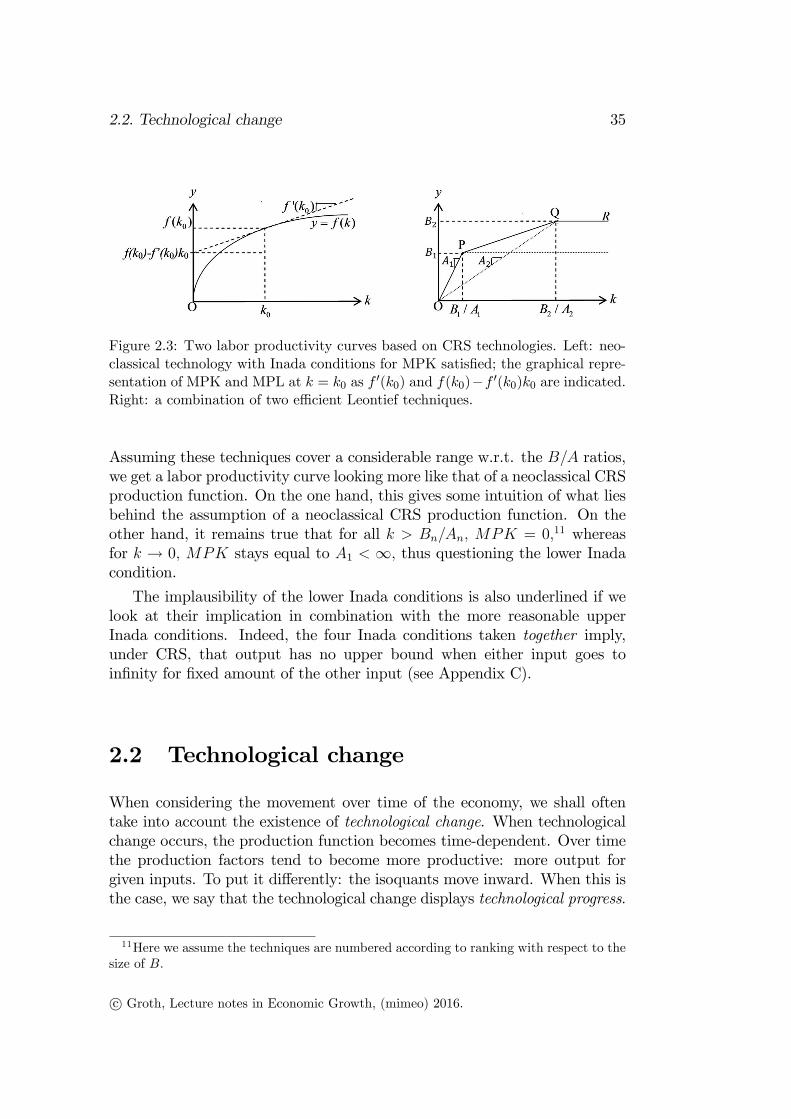
Figure 2.3 is drawn to provide an intuitive understanding of a neoclassicalCRS production function and at the same time illustrate that the lower Inadaconditions are more questionable than the upper Inada conditions. The leftpanel of Figure 2.3 shows output per unit of labor for a CRS neoclassical pro-duction function satisfying the Inada conditions for MPK. The f(k) in thediagram could for instance represent the Cobb-Douglas function in Example1 with β = 1−α, i.e., f(k) = Akα. The right panel of Figure 2.3 shows a non-neoclassical case where only two alternative Leontief techniques are available,technique 1: y = min(A1k,B1), and technique 2: y = min(A2k,B2). In theexposed case it is assumed that B2 > B1 and A2 < A1 (if A2 ≥ A1 at thesame time as B2 > B1, technique 1 would not be effi cient, because the sameoutput could be obtained with less input of at least one of the factors byshifting to technique 2). If the available K and L are such that k < B1/A1
or k > B2/A2, some of either L or K, respectively, is idle. If, however, theavailableK and L are such that B1/A1 < k < B2/A2, it is effi cient to combinethe two techniques and use the fraction µ of K and L in technique 1 and theremainder in technique 2, where µ = (B2/A2 − k)/(B2/A2 −B1/A1). In thisway we get the “labor productivity curve”OPQR (the envelope of the twotechniques) in Figure 2.3. Note that for k → 0, MPK stays equal to A1 <∞,whereas for all k > B2/A2, MPK = 0. A similar feature remains true, whenwe consider many, say n, alternative effi cient Leontief techniques available.
10Given a Cobb-Douglas production function, both production factors are essentialwhether we have DRS, CRS, or IRS.
c© Groth, Lecture notes in Economic Growth, (mimeo) 2016.
2.2. Technological change 35
Figure 2.3: Two labor productivity curves based on CRS technologies. Left: neo-classical technology with Inada conditions for MPK satisfied; the graphical repre-sentation of MPK and MPL at k = k0 as f ′(k0) and f(k0)−f ′(k0)k0 are indicated.Right: a combination of two effi cient Leontief techniques.
Assuming these techniques cover a considerable range w.r.t. the B/A ratios,we get a labor productivity curve looking more like that of a neoclassical CRSproduction function. On the one hand, this gives some intuition of what liesbehind the assumption of a neoclassical CRS production function. On theother hand, it remains true that for all k > Bn/An, MPK = 0,11 whereasfor k → 0, MPK stays equal to A1 < ∞, thus questioning the lower Inadacondition.
The implausibility of the lower Inada conditions is also underlined if welook at their implication in combination with the more reasonable upperInada conditions. Indeed, the four Inada conditions taken together imply,under CRS, that output has no upper bound when either input goes toinfinity for fixed amount of the other input (see Appendix C).
2.2 Technological change
When considering the movement over time of the economy, we shall oftentake into account the existence of technological change. When technologicalchange occurs, the production function becomes time-dependent. Over timethe production factors tend to become more productive: more output forgiven inputs. To put it differently: the isoquants move inward. When this isthe case, we say that the technological change displays technological progress.
11Here we assume the techniques are numbered according to ranking with respect to thesize of B.
c© Groth, Lecture notes in Economic Growth, (mimeo) 2016.

36CHAPTER 2. REVIEW OF TECHNOLOGY AND
FACTOR SHARES OF INCOME
Concepts of neutral technological change
A first step in taking technological change into account is to replace (2.1) by(2.4). Empirical studies often specialize (2.4) by assuming that technologicalchange take a form known as factor-augmenting technological change:
Yt = F (AtKt, BtLt), (2.19)
where F is a (time-independent) neoclassical production function, Yt, Kt,and Lt are output, capital, and labor input, respectively, at time t, while Atand Bt are time-dependent “effi ciencies” of capital and labor, respectively,reflecting technological change.In macroeconomics an even more specific form is often assumed, namely
the form of Harrod-neutral technological change.12 This amounts to assumingthat At in (2.19) is a constant (which we can then normalize to one). So onlyBt, which is then conveniently denoted Tt, is changing over time, and we have
Yt = F (Kt, TtLt). (2.20)
The effi ciency of labor, Tt, is then said to indicate the technology level. Al-though one can imagine natural disasters implying a fall in Tt, generallyTt tends to rise over time and then we say that (2.20) represents Harrod-neutral technological progress. An alternative name often used for this islabor-augmenting technological progress. The names “factor-augmenting”and, as here, “labor-augmenting” have become standard and we shall usethem when convenient, although they may easily be misunderstood. To saythat a change in Tt is labor-augmenting might be understood as meaningthat more labor is required to reach a given output level for given capital.In fact, the opposite is the case, namely that Tt has risen so that less laborinput is required. The idea is that the technological change affects the outputlevel as if the labor input had been increased exactly by the factor by whichT was increased, and nothing else had happened. (We might be tempted tosay that (2.20) reflects “labor saving” technological change. But also thiscan be misunderstood. Indeed, keeping L unchanged in response to a risein T implies that the same output level requires less capital and thus thetechnological change is “capital saving”.)If the function F in (2.20) is homogeneous of degree one (so that the
technology exhibits CRS w.r.t. capital and labor), we may write
yt ≡YtTtLt
= F (Kt
TtLt, 1) = F (kt, 1) ≡ f(kt), f ′ > 0, f ′′ < 0.
12After the English economist Roy F. Harrod, 1900-1978.
c© Groth, Lecture notes in Economic Growth, (mimeo) 2016.

2.2. Technological change 37
where kt ≡ Kt/(TtLt) ≡ kt/Tt (habitually called the “effective” capital in-tensity or, if there is no risk of confusion, just the capital intensity). Inrough accordance with a general trend in aggregate productivity data forindustrialized countries we often assume that T grows at a constant rate, g,so that in discrete time Tt = T0(1 + g)t and in continuous time Tt = T0e
gt,where g > 0. The popularity in macroeconomics of the hypothesis of labor-augmenting technological progress derives from its consistency with Kaldor’s“stylized facts”, cf. Chapter 4.There exists two alternative concepts of neutral technological progress.
Hicks-neutral technological progress is said to occur if technological develop-ment is such that the production function can be written in the form
Yt = TtF (Kt, Lt), (2.21)
where, again, F is a (time-independent) neoclassical production function,while Tt is the growing technology level.13 The assumption of Hicks-neutralityhas been used more in microeconomics and partial equilibrium analysis thanin macroeconomics. If F has CRS, we can write (2.21) as Yt = F (TtKt, TtLt).Comparing with (2.19), we see that in this case Hicks-neutrality is equivalentto At = Bt in (2.19), whereby technological change is said to be equallyfactor-augmenting.Finally, in a symmetric analogy with (2.20), what is known as capital-
augmenting technological progress is present when
Yt = F (TtKt, Lt). (2.22)
Here technological change acts as if the capital input were augmented. Forsome reason this form is sometimes called Solow-neutral technological progress.14
This association of (2.22) to Solow’s name is misleading, however. In his fa-mous growth model,15 Solow assumed Harrod-neutral technological progress.And in another famous contribution, Solow generalized the concept of Harrod-neutrality to the case of embodied technological change and capital of differentvintages, see below.It is easily shown (Exercise I.9) that the Cobb-Douglas production func-
tion (2.8) (with time-independent output elasticities w.r.t. K and L) satisfiesall three neutrality criteria at the same time, if it satisfies one of them (whichit does if technological change does not affect α and β). It can also be shownthat within the class of neoclassical CRS production functions the Cobb-Douglas function is the only one with this property (see Exercise ??).
13After the English economist and Nobel Prize laureate John R. Hicks, 1904-1989.14After the American economist and Nobel Prize laureate Robert Solow (1924-).15Solow (1956).
c© Groth, Lecture notes in Economic Growth, (mimeo) 2016.

38CHAPTER 2. REVIEW OF TECHNOLOGY AND
FACTOR SHARES OF INCOME
Note that the neutrality concepts do not say anything about the sourceof technological progress, only about the quantitative form in which it ma-terializes. For instance, the occurrence of Harrod-neutrality should not beinterpreted as indicating that the technological change emanates specificallyfrom the labor input in some sense. Harrod-neutrality only means that tech-nological innovations predominantly are such that not only do labor andcapital in combination become more productive, but this happens to man-ifest itself in the form (2.20), that is, as if an improvement in the qualityof the labor input had occurred. (Even when improvement in the qualityof the labor input is on the agenda, the result may be a reorganization ofthe production process ending up in a higher Bt along with, or instead of, ahigher At in the expression (2.19).)
Rival versus nonrival goods
When a production function (or more generally a production possibility set)is specified, a given level of technical knowledge is presumed. As this levelchanges over time, the production function changes. In (2.4) this dependencyon the level of knowledge was represented indirectly by the time dependencyof the production function. Sometimes it is useful to let the knowledge de-pendency be explicit by perceiving knowledge as an additional productionfactor and write, for instance,
Yt = F (Xt, Tt), (2.23)
where Tt is now an index of the amount of knowledge, while Xt is a vectorof ordinary inputs like raw materials, machines, labor etc. In this contextthe distinction between rival and nonrival inputs or more generally the dis-tinction between rival and nonrival goods is important. A good is rival ifits character is such that one agent’s use of it inhibits other agents’use ofit at the same time. A pencil is thus rival. Many production inputs likeraw materials, machines, labor etc. have this property. They are elements ofthe vector Xt. By contrast, however, technical knowledge is a nonrival good.An arbitrary number of factories can simultaneously use the same piece oftechnical knowledge in the sense of a list of instructions about how differentinputs can be combined to produce a certain output. An engineering principleor a farmaceutical formula are examples. (Note that the distinction rival-nonrival is different from the distinction excludable-nonexcludable. A goodis excludable if other agents, firms or households, can be excluded from usingit. Other firms can thus be excluded from commercial use of a certain piece oftechnical knowledge if it is patented. The existence of a patent concerns the
c© Groth, Lecture notes in Economic Growth, (mimeo) 2016.

2.2. Technological change 39
legal status of a piece of knowledge and does not interfere with its economiccharacter as a nonrival input.).What the replication argument really says is that by, conceptually, dou-
bling all the rival inputs, we should always be able to double the output,since we just “replicate”what we are already doing. This is then an argu-ment for (at least) CRS w.r.t. the elements of Xt in (2.23). The point is thatbecause of its nonrivalry, we do not need to increase the stock of knowledge.Now let us imagine that the stock of knowledge is doubled at the same timeas the rival inputs are doubled. Then more than a doubling of output shouldoccur. In this sense we may speak of IRS w.r.t. the rival inputs and T takentogether.Before proceeding, we briefly comment on how the capital stock, Kt,
is typically measured. While data on gross investment, It, is available innational income and product accounts, data on Kt usually is not. One ap-proach to the measurement of Kt is the perpetual inventory method whichbuilds upon the accounting relationship
Kt = It−1 + (1− δ)Kt−1. (2.24)
Assuming a constant capital depreciation rate δ, backward substitution gives
Kt = It−1+(1−δ) [It−2 + (1− δ)Kt−2] = . . . =N∑i=1
(1−δ)i−1It−i+(1−δ)NKt−N .
(2.25)Based on a long time series for I and an estimate of δ, one can insert theseobserved values in the formula and calculate Kt, starting from a rough con-jecture about the initial value Kt−N . The result will not be very sensitive tothis conjecture since for large N the last term in (2.25) becomes very small.
Embodied vs. disembodied technological progress
There exists an additional taxonomy of technological change. We say thattechnological change is embodied, if taking advantage of new technical knowl-edge requires construction of new investment goods. The new technology isincorporated in the design of newly produced equipment, but this equipmentwill not participate in subsequent technological progress. An example: onlythe most recent vintage of a computer series incorporates the most recentadvance in information technology. Then investment goods produced later(investment goods of a later “vintage”) have higher productivity than in-vestment goods produced earlier at the same resource cost. Thus investmentbecomes an important driving force in productivity increases.
c© Groth, Lecture notes in Economic Growth, (mimeo) 2016.

40CHAPTER 2. REVIEW OF TECHNOLOGY AND
FACTOR SHARES OF INCOME
We way formalize embodied technological progress by writing capital ac-cumulation in the following way:
Kt+1 −Kt = qtIt − δKt, (2.26)
where It is gross investment in period t, i.e., It = Yt − Ct, and qt measuresthe “quality”(productivity) of newly produced investment goods. The risinglevel of technology implies rising q so that a given level of investment givesrise to a greater and greater addition to the capital stock, K, measuredin effi ciency units. In aggregate models C and I are produced with thesame technology, the aggregate production function. From this together with(2.26) follows that q capital goods can be produced at the same minimumcost as one consumption good. Hence, the equilibrium price, p, of capitalgoods in terms of the consumption good must equal the inverse of q, i.e.,p = 1/q. The output-capital ratio in value terms is Y/(pK) = qY/K.Note that even if technological change does not directly appear in the
production function, that is, even if for instance (2.20) is replaced by Yt= F (Kt, Lt), the economy may experience a rising standard of living when qis growing over time.In contrast, disembodied technological change occurs when new technical
and organizational knowledge increases the combined productivity of the pro-duction factors independently of when they were constructed or educated. IftheKt appearing in (2.20), (2.21), and (2.22) above refers to the total, histor-ically accumulated capital stock as calculated by (2.25), then the evolutionof T in these expressions can be seen as representing disembodied technolog-ical change. All vintages of the capital equipment benefit from a rise in thetechnology level Tt. No new investment is needed to benefit.Based on data for the U.S. 1950-1990, and taking quality improvements
into account, Greenwood et al. (1997) estimate that embodied technologicalprogress explains about 60% of the growth in output per man hour. So,empirically, embodied technological progress seems to play a dominant role.As this tends not to be fully incorporated in national income accounting atfixed prices, there is a need to adjust the investment levels in (2.25) to bettertake estimated quality improvements into account. Otherwise the resultingK will not indicate the capital stock measured in effi ciency units.
2.3 The concepts of representative firm andaggregate production function*
Many macroeconomic models make use of the simplifying notion of a rep-resentative firm. By this is meant a fictional firm whose production “rep-
c© Groth, Lecture notes in Economic Growth, (mimeo) 2016.

2.3. The concepts of representative firm and aggregate production function*41
resents” aggregate production (value added) in a sector or in society as awhole.Suppose there are n firms in the sector considered or in society as a
whole. Let F i be the production function for firm i so that Yi = F i(Ki, Li),where Yi, Ki, and Li are output, capital input, and labor input, respectively,i = 1, 2, . . . , n. Further, let Y = Σn
i=1Yi, K = Σni=1Ki, and L = Σn
i=1Li.Ignoring technological change, suppose the aggregate variables are relatedthrough some function, F ∗, such that we can write
Y = F ∗(K,L),
and such that the choices of a single firm facing this production functioncoincide with the aggregate outcomes, Σn
i=1Yi, Σni=1Ki, and Σn
i=1Li, in theoriginal economy. Then F ∗(K,L) is called the aggregate production functionor the production function of the representative firm. It is as if aggregateproduction is the result of the behavior of such a single firm.A simple example where the aggregate production function is well-defined
is the following. Suppose that all firms have the same production functionso that Yi = F (Ki, Li), i = 1, 2, . . . , n. If in addition F has CRS, we have
Yi = F (Ki, Li) = LiF (ki, 1) ≡ Lif(ki),
where ki ≡ Ki/Li. Hence, facing given factor prices, cost-minimizing firmswill choose the same capital intensity ki = k for all i. From Ki = kLi thenfollows
∑iKi = k
∑i Li so that k = K/L. Thence,
Y ≡∑
Yi =∑
Lif(ki) = f(k)∑
Li = f(k)L = F (k, 1)L = F (K,L).
In this (trivial) case the aggregate production function is well-defined andturns out to be exactly the same as the identical CRS production functionsof the individual firms. Moreover, given CRS and ki = k for all i, we have∂Yi/∂Ki = f ′(ki) = f ′(k) = FK(K,L) for all i. So each firm’s marginalproductivity of capital is the same as the marginal productivity of capital onthe basis of the aggregate production function.Allowing for the existence of different production functions at firm level,
we may define the aggregate production function as
F (K,L) = max(K1,L1,...,Kn,Ln)≥0
F 1(K1, L1) + · · ·+ F n(Kn, Ln)
s.t.∑i
Ki ≤ K,∑i
Li ≤ L.
Allowing also for existence of different output goods, different capitalgoods, and different types of labor makes the issue more intricate, of course.
c© Groth, Lecture notes in Economic Growth, (mimeo) 2016.

42CHAPTER 2. REVIEW OF TECHNOLOGY AND
FACTOR SHARES OF INCOME
Yet, if firms are price taking profit maximizers and there are nonincreasingreturns to scale, we at least know that the aggregate outcome is as if, forgiven prices, the firms jointly maximize aggregate profit on the basis of theircombined production technology (Mas-Colell et al., 1955). The problem is,however, that the conditions needed for this to imply existence of an ag-gregate production function which is well-behaved (in the sense of inheritingsimple qualitative properties from its constituent parts) are restrictive.Nevertheless macroeconomics often treats aggregate output as a single ho-
mogeneous good and capital and labor as being two single and homogeneousinputs. There was in the 1960s a heated debate about the problems involvedin this, with particular emphasis on the aggregation of different kinds ofequipment into one variable, the capital stock “K”. The debate is knownas the “Cambridge controversy”because the dispute was between a group ofeconomists from Cambridge University, UK, and a group from MassachusettsInstitute of Technology (MIT), which is located in Cambridge, USA. The for-mer group questioned the theoretical robustness of several of the neoclassicaltenets, including the proposition that rising aggregate capital intensity tendsto be associated with a falling rate of interest. Starting at the disaggregatelevel, an association of this sort is not a logical necessity because, with differ-ent production functions across the industries, the relative prices of producedinputs tend to change, when the interest rate changes. While acknowledgingthe possibility of “paradoxical” relationships, the latter group maintainedthat in a macroeconomic context they are likely to cause devastating prob-lems only under exceptional circumstances. In the end this is a matter ofempirical assessment.16
To avoid complexity and because, for many important issues in growththeory, there is today no well-tried alternative, we shall in this course mostof the time use aggregate constructs like “Y ”, “K”, and “L” as simplify-ing devices, hopefully acceptable in a first approximation. There are cases,however, where some disaggregation is pertinent. When for example the roleof imperfect competition is in focus, we shall be ready to disaggregate theproduction side of the economy into several product lines, each producing itsown differentiated product. We shall also touch upon a type of growth modelswhere a key ingredient is the phenomenon of “creative destruction”meaningthat an incumbent technological leader is competed out by an entrant witha qualitatively new technology.Like the representative firm, the representative household and the aggre-
16In his review of the Cambridge controversy Mas-Colell (1989) concluded that: “Whatthe ‘paradoxical’ comparative statics [of disaggregate capital theory] has taught us issimply that modelling the world as having a single capital good is not a priori justified.So be it.”
c© Groth, Lecture notes in Economic Growth, (mimeo) 2016.

2.4. Long-run vs. short-run production functions* 43
gate consumption function are simplifying notions that should be appliedonly when they do not get in the way of the issue to be studied. The im-portance of budget constraints may make it even more diffi cult to aggregateover households than over firms. Yet, if (and that is a big if) all householdshave the same, constant marginal propensity to consume out of income, ag-gregation is straightforward and the representative household is a meaningfulconcept. On the other hand, if we aim at understanding, say, the interactionbetween lending and borrowing households, perhaps via financial intermedi-aries, the representative household is not a useful starting point. Similarly,if the theme is conflicts of interests between firm owners and employees, theexistence of different types of households should be taken into account.
2.4 Long-run vs. short-run production func-tions*
Is the substitutability between capital and labor the same “ex ante”and “expost”? By ex ante is meant “when plant and machinery are to be decidedupon”and by ex post is meant “after the equipment is designed and con-structed”. In the standard neoclassical competitive setup, of for instancethe Solow or the Ramsey model, there is a presumption that also after theconstruction and installation of the equipment in the firm, the ratio of thefactor inputs can be fully adjusted to a change in the relative factor price. Inpractice, however, when some machinery has been constructed and installed,its functioning will often require a more or less fixed number of machine op-erators. What can be varied is just the degree of utilization of the machinery.That is, after construction and installation of the machinery, the choice op-portunities are no longer described by the neoclassical production functionbut by a Leontief production function,
Y = min(AuK,BL), A > 0, B > 0, (2.27)
where K is the size of the installed machinery (a fixed factor in the shortrun) measured in effi ciency units, u is its utilization rate (0 ≤ u ≤ 1), and Aand B are given technical coeffi cients measuring effi ciency.So in the short run the choice variables are u and L. In fact, essentially
only u is a choice variable since effi cient production trivially requires L =AuK/B. Under “full capacity utilization”we have u = 1 (each machine isused 24 hours per day seven days per week). “Capacity”is given as AK perweek. Producing effi ciently at capacity requiresL = AK/B and the marginalproduct by increasing labor input is here nil. But if demand, Y d, is less than
c© Groth, Lecture notes in Economic Growth, (mimeo) 2016.

44CHAPTER 2. REVIEW OF TECHNOLOGY AND
FACTOR SHARES OF INCOME
capacity, satisfying this demand effi ciently requires u = Y d/(AK) < 1 and L= Y d/B. As long as u < 1, the marginal productivity of labor is a constant,B.The various effi cient input proportions that are possible ex ante may be
approximately described by a neoclassical CRS production function. Let thisfunction on intensive form be denoted y = f(k).When investment is decidedupon and undertaken, there is thus a choice between alternative effi cient pairsof the technical coeffi cients A and B in (2.27). These pairs satisfy
f(k) = Ak = B. (2.28)
So, for an increasing sequence of k’s, k1, k2,. . . , ki,. . . , the correspondingpairs are (Ai, Bi) = (f(ki)/ki, f(ki)), i = 1, 2,. . . .17 We say that ex ante,depending on the relative factor prices as they are “now”and are expectedto evolve in the future, a suitable technique, (Ai, Bi), is chosen from anopportunity set described by the given neoclassical production function. Butex post, i.e., when the equipment corresponding to this technique is installed,the production opportunities are described by a Leontief production functionwith (A,B) = (Ai, Bi).In the picturesque language of Phelps (1963), technology is in this case
putty-clay. Ex ante the technology involves capital which is “putty” in thesense of being in a malleable state which can be transformed into a range ofvarious machinery requiring capital-labor ratios of different magnitude. Butonce the machinery is constructed, it enters a “hardened”state and becomes”clay”. Then factor substitution is no longer possible; the capital-labor ra-tio at full capacity utilization is fixed at the level k = Bi/Ai, as in (2.27).Following the terminology of Johansen (1972), we say that a putty-clay tech-nology involves a “long-run production function”which is neoclassical and a“short-run production function”which is Leontief.In contrast, the standard neoclassical setup assumes the same range of
substitutability between capital and labor ex ante and ex post. Then thetechnology is called putty-putty. This term may also be used if ex post thereis at least some substitutability although less than ex ante. At the oppositepole of putty-putty we may consider a technology which is clay-clay. Hereneither ex ante nor ex post is factor substitution possible. Table 2.1 gives anoverview of the alternative cases.
Table 2.1. Technologies classified according to
17The points P and Q in the right-hand panel of Fig. 2.3 can be interpreted as con-structed this way from the neoclassical production function in the left-hand panel of thefigure.
c© Groth, Lecture notes in Economic Growth, (mimeo) 2016.

2.5. The neoclassical theory of factor income shares 45
factor substitutability ex ante and ex postEx post substitution
Ex ante substitution possible impossiblepossible putty-putty putty-clayimpossible clay-clay
The putty-clay case is generally considered the realistic case. As timeproceeds, technological progress occurs. To take this into account, we mayreplace (2.28) and (2.27) by f(kt, t) = Atkt = Bt and Yt = min(AtutKt, BtLt),respectively. If a new pair of Leontief coeffi cients, (At2 , Bt2), effi ciency-dominates its predecessor (by satisfying At2 ≥ At1 and Bt2 ≥ Bt1 with atleast one strict equality), it may pay the firm to invest in the new technol-ogy at the same time as some old machinery is scrapped. Real wages tendto rise along with technological progress and the scrapping occurs becausethe revenue from using the old machinery in production no longer covers theassociated labor costs.The clay property ex-post of many technologies is important for short-run
analysis. It implies that there may be non-decreasing marginal productivityof labor up to a certain point. It also implies that in its investment decisionthe firm will have to take expected future technologies and future factor pricesinto account. For many issues in long-run analysis the clay property ex-postmay be less important, since over time adjustment takes place through newinvestment.
2.5 The neoclassical theory of factor incomeshares
To begin with, we ignore technological progress and write aggregate outputas Y = F (K,L), where F is neoclassical with CRS. From Euler’s theoremfollows that F (K,L) = F1K + F2L = f ′(k)K + (f(k) − kf ′(k))L, wherek ≡ K/L. In equilibrium under perfect competition we have
Y = rK + wL,
where r = r + δ = f ′(k) ≡ r(k) is the cost per unit of capital input and w= f(k)−kf ′(k) ≡ w(k) is the real wage, i.e., the cost per unit of labor input.We have r′(k) = f ′′(k) < 0 and w′(k) = −kf ′′(k) > 0.The labor income share is
wL
Y=f(k)− kf ′(k)
f(k)≡ w(k)
f(k)≡ SL(k) =
wL
rK + wL=
w/rk
1 + w/rk
, (2.29)
c© Groth, Lecture notes in Economic Growth, (mimeo) 2016.

46CHAPTER 2. REVIEW OF TECHNOLOGY AND
FACTOR SHARES OF INCOME
where the function SL(·) is the income share of labor function, w/r is thefactor price ratio, and (w/r)/k = w/(rk) is the factor income ratio. As r′(k)= f ′′(k) < 0 and w′(k) = −kf ′′(k) > 0, the factor price ratio, w/r, is anincreasing function of k.Suppose that capital tends to grow faster than labor so that k rises over
time. Unless the production function is Cobb-Douglas, this will under perfectcompetition affect the labor income share. But apriori it is not obvious inwhat direction. By (2.29) we see that the labor income share moves inthe same direction as the factor income ratio, (w/r)/k. The latter goes up(down) depending on whether the percentage rise in the factor price ratiow/r is greater (smaller) than the percentage rise in k. So, if we let E`xg(x)denote the elasticity of a function g(x) w.r.t. x, we can only say that
SL′(k) R 0 for E`kw
rR 1, (2.30)
respectively. In words: if the production function is such that the ratio ofthe marginal productivities of the two production factors is strongly (weakly)sensitive to the capital-labor ratio, then the labor income share rises (falls)along with a rise in K/L.Usually, however, the inverse elasticity is considered, namely E`w/rk (=
1/E`k wr ). This elasticity indicates how sensitive the cost minimizing capital-labor ratio, k, is to a given factor price ratio w/r. Under perfect competitionE`w/rk coincides with what is known as the elasticity of factor substitution(for a general definition, see below). The latter is often denoted σ. In theCRS case, σ will be a function of only k so that we can write E`w/rk = σ(k).By (2.30), we therefore have
SL′(k) R 0 for σ(k) Q 1,
respectively.The size of the elasticity of factor substitution is a property of the pro-
duction function, hence of the technology. In special cases the elasticity offactor substitution is a constant, i.e., independent of k. For instance, if F isCobb-Douglas, i.e., Y = KαL1−α, 0 < α < 1, we have σ(k) ≡ 1, as shownin Section 2.7. In this case variation in k does not change the labor incomeshare under perfect competition. Empirically there is not agreement aboutthe “normal” size of the elasticity of factor substitution for industrializedeconomies, but the bulk of studies seems to conclude with σ(k) < 1 (seebelow).
Adding Harrod-neutral technical progress We now add Harrod-neutraltechnical progress. We write aggregate output as Y = F (K,TL), where F
c© Groth, Lecture notes in Economic Growth, (mimeo) 2016.
2.5. The neoclassical theory of factor income shares 47
is neoclassical with CRS, and T = Tt = T0(1 + g)t. Then the labor incomeshare is
wL
Y=
w/T
Y/(TL)≡ w
y.
The above formulas still hold if we replace k by k ≡ K/(TL) and w by w≡ w/T. We get
SL′(k) R 0 for σ(k) Q 1,
respectively. We see that if σ(k) < 1 in the relevant range for k, then marketforces tend to increase the income share of the factor that is becoming rela-tively more scarce, which is effi ciency-adjusted labor, TL, if k is increasing.And if instead σ(k) > 1 in the relevant range for k, then market forces tendto decrease the income share of the factor that is becoming relatively morescarce.While k empirically is clearly growing, k ≡ k/T is not necessarily so
because also T is increasing. Indeed, according to Kaldor’s “stylized facts”,apart from short- and medium-term fluctuations, k − and therefore also rand the labor income share − tend to be more or less constant over time.This can happen whatever the sign of σ(k∗) − 1, where k∗ is the long-runvalue of the effective capital-labor ratio k. Given CRS and the productionfunction f, the elasticity of substitution between capital and labor does notdepend on whether g = 0 or g > 0, but only on the function f itself and thelevel of K/(TL).As alluded to earlier, there are empiricists who reject Kaldor’s “facts”
as a general tendency. For instance Piketty (2014) essentially claims thatin the very long run the effective capital-labor ratio k has an upward trend,temporarily braked by two world wars and the Great Depression in the 1930s.If so, the sign of σ(k)− 1 becomes decisive for in what direction wL/Y willmove. Piketty interprets the econometric literature as favoring σ(k) > 1,which means there should be downward pressure on wL/Y . This particularsource behind a falling wL/Y can be questioned, however. Indeed, σ(k) > 1contradicts the more general empirical view referred to above.18
Immigration
Here is another example that illustrates the importance of the size of σ(k).Consider an economy with perfect competition and a given aggregate capitalstock K and technology level T (entering the production function in thelabor-augmenting way as above). Suppose that for some reason, immigration,
18According to Summers (2014), Piketty’s interpretation relies on conflating gross andnet returns to capital.
c© Groth, Lecture notes in Economic Growth, (mimeo) 2016.

48CHAPTER 2. REVIEW OF TECHNOLOGY AND
FACTOR SHARES OF INCOME
say, aggregate labor supply, L, shifts up and full employment is maintainedby the needed real wage adjustment. Given the present model, in whatdirection will aggregate labor income wL = w(k)TL then change? The effectof the larger L is to some extent offset by a lower w brought about by thelower effective capital-labor ratio. Indeed, in view of dw/dk = −kf ′′(k) > 0,we have k ↓ implies w ↓ for fixed T. So we cannot apriori sign the change inwL. The following relationship can be shown (Exercise ??), however:
∂(wL)
∂L= (1− α(k)
σ(k))w R 0 for α(k) Q σ(k), (2.31)
respectively, where a(k) ≡ kf ′(k)/f(k) is the output elasticity w.r.t. capitalwhich under perfect competition equals the gross capital income share. Itfollows that the larger L will not be fully offset by the lower w as long as theelasticity of factor substitution, σ(k), exceeds the gross capital income share,α(k). This condition seems confirmed by most of the empirical evidence (seeSection 2.7).The next section describes the concept of the elasticity of factor substitu-
tion at a more general setting. The subsequent section introduces the specialcase known as the CES production function.
2.6 The elasticity of factor substitution*
We shall here discuss the concept of elasticity of factor substitution at amore general level. Fig. 2.4 depicts an isoquant, F (K,L) = Y , for a givenneoclassical production function, F (K,L), which need not have CRS. LetMRS denote the marginal rate of substitution of K for L, i.e., MRS =FL(K,L)/FK(K,L).19 At a given point (K,L) on the isoquant curve, MRSis given by the absolute value of the slope of the tangent to the isoquant atthat point. This tangent coincides with that isocost line which, given thefactor prices, has minimal intercept with the vertical axis while at the sametime touching the isoquant. In view of F (·) being neoclassical, the isoquantsare by definition strictly convex to the origin. Consequently, MRS is risingalong the curve when L decreases and thereby K increases. Conversely, wecan let MRS be the independent variable and consider the correspondingpoint on the indifference curve, and thereby the ratio K/L, as a function ofMRS. If we let MRS rise along the given isoquant, the corresponding valueof the ratio K/L will also rise.
19When there is no risk of confusion as to what is up and what is down, we use MRSas a shorthand for the more precise expression MRSKL.
c© Groth, Lecture notes in Economic Growth, (mimeo) 2016.

2.6. The elasticity of factor substitution* 49
Figure 2.4: Substitution of capital for labor as the marginal rate of substitutionincreases from MRS to MRS′.
The elasticity of substitution between capital and labor is defined as theelasticity of the ratio K/L with respect to MRS when we move along agiven isoquant, evaluated at the point (K,L). Let this elasticity be denotedσ(K,L). Thus,
σ(K,L) =MRS
K/L
d(K/L)
dMRS |Y=Y=
d(K/L)K/L
dMRSMRS |Y=Y
. (2.32)
Although the elasticity of factor substitution is a characteristic of the tech-nology as such and is here defined without reference to markets and factorprices, it helps the intuition to refer to factor prices. At a cost-minimizingpoint, MRS equals the factor price ratio w/r. Thus, the elasticity of fac-tor substitution will under cost minimization coincide with the percentageincrease in the ratio of the cost-minimizing factor ratio induced by a onepercentage increase in the inverse factor price ratio, holding the output levelunchanged.20 The elasticity of factor substitution is thus a positive numberand reflects how sensitive the capital-labor ratioK/L is under cost minimiza-tion to an increase in the factor price ratio w/r for a given output level. Theless curvature the isoquant has, the greater is the elasticity of factor substitu-tion. In an analogue way, in consumer theory one considers the elasticity ofsubstitution between two consumption goods or between consumption todayand consumption tomorrow. In that context the role of the given isoquant
20This characterization is equivalent to interpreting the elasticity of substitution as thepercentage decrease in the factor ratio (when moving along a given isoquant) induced bya one-percentage increase in the corresponding factor price ratio.
c© Groth, Lecture notes in Economic Growth, (mimeo) 2016.

50CHAPTER 2. REVIEW OF TECHNOLOGY AND
FACTOR SHARES OF INCOME
is taken over by an indifference curve. That is also the case when we con-sider the intertemporal elasticity of substitution in labor supply, cf. the nextchapter.Calculating the elasticity of substitution between K and L at the point
(K,L), we get
σ(K,L) = − FKFL(FKK + FLL)
KL [(FL)2FKK − 2FKFLFKL + (FK)2FLL], (2.33)
where all the derivatives are evaluated at the point (K,L). When F (K,L)has CRS, the formula (2.33) simplifies to
σ(K,L) =FK(K,L)FL(K,L)
FKL(K,L)F (K,L)= −f
′(k) (f(k)− f ′(k)k)
f ′′(k)kf(k)≡ σ(k), (2.34)
where k ≡ K/L.21 We see that under CRS, the elasticity of substitutiondepends only on the capital-labor ratio k, not on the output level. We willnow consider the case where the elasticity of substitution is independent alsoof the capital-labor ratio.
2.7 The CES production function
It can be shown22 that if a neoclassical production function with CRS has aconstant elasticity of factor substitution different from one, it must be of theform
Y = A[αKβ + (1− α)Lβ
] 1β , (2.35)
where A, α, and β are parameters satisfying A > 0, 0 < α < 1, and β < 1,β 6= 0. This function has been used intensively in empirical studies and iscalled a CES production function (CES for Constant Elasticity of Substitu-tion). For a given choice of measurement units, the parameter A reflectseffi ciency (or what is known as total factor productivity) and is thus calledthe effi ciency parameter. The parameters α and β are called the distribu-tion parameter and the substitution parameter, respectively. The restrictionβ < 1 ensures that the isoquants are strictly convex to the origin. Note thatif β < 0, the right-hand side of (16.32) is not defined when either K or L(or both) equal 0.We can circumvent this problem by extending the domainof the CES function and assign the function value 0 to these points whenβ < 0. Continuity is maintained in the extended domain (see Appendix E).
21The formulas (2.33) and (2.34) are derived in Appendix D of Chapter 4 of Groth,Lecture Notes in Macroeconomics..22See, e.g., Arrow et al. (1961).
c© Groth, Lecture notes in Economic Growth, (mimeo) 2016.

2.7. The CES production function 51
By taking partial derivatives in (16.32) and substituting back we get
∂Y
∂K= αAβ
(Y
K
)1−β
and∂Y
∂L= (1− α)Aβ
(Y
L
)1−β
, (2.36)
where Y/K = A[α + (1− α)k−β
] 1β and Y/L = A
[αkβ + 1− α
] 1β . The mar-
ginal rate of substitution of K for L therefore is
MRS =∂Y/∂L
∂Y/∂K=
1− αα
k1−β > 0.
Consequently,dMRS
dk=
1− αα
(1− β)k−β,
where the inverse of the right-hand side is the value of dk/dMRS. Substitut-ing these expressions into (16.34) gives
σ(K,L) =1
1− β ≡ σ, (2.37)
confirming the constancy of the elasticity of substitution. Since β < 1, σ > 0always. A higher substitution parameter, β, results in a higher elasticity offactor substitution, σ. And σ ≶ 1 for β ≶ 0, respectively.Since β = 0 is not allowed in (16.32), at first sight we cannot get σ = 1
from this formula. Yet, σ = 1 can be introduced as the limiting case of (16.32)when β → 0, which turns out to be the Cobb-Douglas function. Indeed, onecan show23 that, for fixed K and L,
A[αKβ + (1− α)Lβ
] 1β → AKαL1−α, for β → 0.
By a similar procedure as above we find that a Cobb-Douglas function alwayshas elasticity of substitution equal to 1; this is exactly the value taken byσ in (16.35) when β = 0. In addition, the Cobb-Douglas function is theonly production function that has unit elasticity of substitution whateverthe capital-labor ratio.Another interesting limiting case of the CES function appears when, for
fixed K and L, we let β → −∞ so that σ → 0. We get
A[αKβ + (1− α)Lβ
] 1β → Amin(K,L), for β → −∞. (2.38)
23For proofs of this and the further claims below, see Appendix E of Chapter 4 of Groth,Lecture Notes in Macroeconomics.
c© Groth, Lecture notes in Economic Growth, (mimeo) 2016.

52CHAPTER 2. REVIEW OF TECHNOLOGY AND
FACTOR SHARES OF INCOME
So in this case the CES function approaches a Leontief production function,the isoquants of which form a right angle, cf. Fig. 2.5. In the limit there is nopossibility of substitution between capital and labor. In accordance with thisthe elasticity of substitution calculated from (16.35) approaches zero when βgoes to −∞.Finally, let us consider the “opposite”transition. For fixed K and L we
let the substitution parameter rise towards 1 and get
A[αKβ + (1− α)Lβ
] 1β → A [αK + (1− α)L] , for β → 1.
Here the elasticity of substitution calculated from (16.35) tends to ∞ andthe isoquants tend to straight lines with slope −(1 − α)/α. In the limit,the production function thus becomes linear and capital and labor becomeperfect substitutes.
0 1 2 3 4 5 6 7
1
2
3
4
5
σ = 0
σ = 0.5
σ = 1σ = 1.5
σ = ∞2A
2A
2Aα
2A(1−α)
L
K
Figure 2.5: Isoquants for the CES function for alternative values of σ (A = 1.5,Y = 2, and α = 0.42).
Fig. 2.5 depicts isoquants for alternative CES production functions andtheir limiting cases. In the Cobb-Douglas case, σ = 1, the horizontal andvertical asymptotes of the isoquant coincide with the coordinate axes. Whenσ < 1, the horizontal and vertical asymptotes of the isoquant belong to theinterior of the positive quadrant. This implies that both capital and labor
c© Groth, Lecture notes in Economic Growth, (mimeo) 2016.
2.7. The CES production function 53
are essential inputs. When σ > 1, the isoquant terminates in points onthe coordinate axes. Then neither capital, nor labor are essential inputs.Empirically there is not complete agreement about the “normal”size of theelasticity of factor substitution for industrialized economies. The elasticityalso differs across the production sectors. A thorough econometric study(Antràs, 2004) of U.S. data indicate the aggregate elasticity of substitutionto be in the interval (0.5, 1.0). The survey by Chirinko (2008) concludes withthe interval (0.4, 0.6). Starting from micro data, a recent study by Oberfieldand Raval (2014) finds that the elasticity of factor substitution for the USmanufacturing sector as a whole has been stable since 1970 at about 0.7.
The CES production function in intensive form
Dividing through by L on both sides of (16.32), we obtain the CES productionfunction in intensive form,
y ≡ Y
L= A(αkβ + 1− α)
1β , (2.39)
where k ≡ K/L. The marginal productivity of capital can be written
MPK =dy
dk= αA
[α + (1− α)k−β
] 1−ββ = αAβ
(yk
)1−β,
which of course equals ∂Y/∂K in (16.33). We see that the CES functionviolates either the lower or the upper Inada condition for MPK, dependingon the sign of β. Indeed, when β < 0 (i.e., σ < 1), then for k → 0 both y/kand dy/dk approach an upper bound equal to Aα1/β < ∞, thus violatingthe lower Inada condition for MPK (see the right-hand panel of Fig. 2.3).It is also noteworthy that in this case, for k → ∞, y approaches an upperbound equal to A(1 − α)1/β < ∞. These features reflect the low degree ofsubstitutability when β < 0.When instead β > 0, there is a high degree of substitutability (σ > 1).
Then, for k →∞ both y/k and dy/dk → Aα1/β > 0, thus violating the upperInada condition forMPK (see right panel of Fig. 2.6). It is also noteworthythat for k → 0, y approaches a positive lower bound equal to A(1−α)1/β > 0.Thus, in this case capital is not essential. At the same time dy/dk →∞ fork → 0 (so the lower Inada condition for the marginal productivity of capitalholds). Details are in Appendix E.The marginal productivity of labor is
MPL =∂Y
∂L= (1− α)Aβy1−β = (1− α)A(αkβ + 1− α)(1−β)/β ≡ w(k),
c© Groth, Lecture notes in Economic Growth, (mimeo) 2016.

54CHAPTER 2. REVIEW OF TECHNOLOGY AND
FACTOR SHARES OF INCOME
from (16.33).Since (16.32) is symmetric inK and L, we get a series of symmetric results
by considering output per unit of capital as x≡ Y/K = A[α + (1− α)(L/K)β
]1/β.
In total, therefore, when there is low substitutability (β < 0), for fixed inputof either of the production factors, there is an upper bound for how muchan unlimited input of the other production factor can increase output. Andwhen there is high substitutability (β > 0), there is no such bound and anunlimited input of either production factor take output to infinity.The Cobb-Douglas case, i.e., the limiting case for β → 0, constitutes in
several respects an intermediate case in that all four Inada conditions aresatisfied and we have y → 0 for k → 0, and y →∞ for k →∞.
0 5 10
5
A (1 − α)1β
∆x ·Aα1β
∆x
a) The case of σ < 1.
k
y
0 5 10
5
A (1 − α)1β
∆x ·Aα1β
∆x
a) The case of σ > 1.
k
y
Figure 2.6: The CES production function in intensive form, σ = 1/(1− β), β < 1.
Generalizations
The CES production function considered above has CRS. By adding an elas-ticity of scale parameter, γ, we get the generalized form
Y = A[αKβ + (1− α)Lβ
] γβ , γ > 0. (2.40)
In this form the CES function is homogeneous of degree γ. For 0 < γ < 1,there are DRS, for γ = 1 CRS, and for γ > 1 IRS. If γ 6= 1, it may beconvenient to consider Q ≡ Y 1/γ = A1/γ
[αKβ + (1− α)Lβ
]1/βand q ≡ Q/L
= A1/γ(αkβ + 1− α)1/β.The elasticity of substitution between K and L is σ = 1/(1−β) whatever
the value of γ. So including the limiting cases as well as non-constant returnsto scale in the “family”of production functions with constant elasticity ofsubstitution, we have the simple classification displayed in Table 2.2.
c© Groth, Lecture notes in Economic Growth, (mimeo) 2016.

2.8. Literature notes 55
Table 2.2 The family of production functionswith constant elasticity of substitution.
σ = 0 0 < σ < 1 σ = 1 σ > 1Leontief CES Cobb-Douglas CES
Note that only for γ ≤ 1 is (16.38) a neoclassical production function.This is because, when γ > 1, the conditions FKK < 0 and FNN < 0 do nothold everywhere.We may generalize further by assuming there are n inputs, in the amounts
X1, X2, ..., Xn. Then the CES production function takes the form
Y = A[α1X1
β + α2X2β + ...αnXn
β] γβ , αi > 0 for all i,
∑i
αi = 1, γ > 0.
(2.41)In analogy with (16.34), for an n-factor production function the partial elas-ticity of substitution between factor i and factor j is defined as
σij =MRSijXi/Xj
d(Xi/Xj)
dMRSij |Y=Y
,
where it is understood that not only the output level but also all Xk, k 6= i, j,are kept constant. Note that σji = σij. In the CES case considered in (16.39),all the partial elasticities of substitution take the same value, 1/(1− β).
2.8 Literature notes
As to the question of the empirical validity of the constant returns to scaleassumption, Malinvaud (1998) offers an account of the econometric diffi cul-ties associated with estimating production functions. Studies by Basu (1996)and Basu and Fernald (1997) suggest returns to scale are about constant ordecreasing. Studies by Hall (1990), Caballero and Lyons (1992), Harris andLau (1992), Antweiler and Treffl er (2002), and Harrison (2003) suggest thereare quantitatively significant increasing returns, either internal or external.On this background it is not surprising that the case of IRS (at least at in-dustry level), together with market forms different from perfect competition,has in recent years received more attention in macroeconomics and in thetheory of economic growth.Macroeconomists’use of the value-laden term “technological progress”in
connection with technological change may seem suspect. But the term shouldbe interpreted as merely a label for certain types of shifts of isoquants in an
c© Groth, Lecture notes in Economic Growth, (mimeo) 2016.

56CHAPTER 2. REVIEW OF TECHNOLOGY AND
FACTOR SHARES OF INCOME
abstract universe. At a more concrete and disaggregate level analysts ofcourse make use of more refined notions about technological change, recog-nizing for example not only benefits of new technologies, but also the risks,including risk of fundamental mistakes (think of the introduction and laterabandonment of asbestos in the construction industry).Informative history of technology is contained in Ruttan (2001) and Smil
(2003). For more general economic history, see, e.g., Clark (2008) and Pers-son (2010). Forecasts of technological development in the next decades arecontained in, for instance, Brynjolfsson and McAfee (2014).Embodied technological progress, sometimes called investment-specific
technological progress, is explored in, for instance, Solow (1960), Greenwoodet al. (1997), and Groth and Wendner (2014). Hulten (2001) surveys theliterature and issues related to measurement of the direct contribution ofcapital accumulation and technological change, respectively, to productivitygrowth.Conditions ensuring that a representative household is admitted and the
concept of Gorman preferences are discussed in Acemoglu (2009). Anotheruseful source, also concerning the conditions for the representative firm to bea meaningful notion, is Mas-Colell et al. (1995). For general discussions of thelimitations of representative agent approaches, see Kirman (1992) and Galle-gati and Kirman (1999). Reviews of the “Cambridge Controversy”are con-tained in Mas-Colell (1989) and Felipe and Fisher (2003). The last-mentionedauthors find the conditions required for the well-behavedness of these con-structs so stringent that it is diffi cult to believe that actual economies arein any sense close to satisfy them. For a less distrustful view, see for in-stance Ferguson (1969), Johansen (1972), Malinvaud (1998), Jorgenson et al.(2005), and Jones (2005).It is often assumed that capital depreciation can be described as geomet-
ric (in continuous time exponential) evaporation of the capital stock. Thisformula is popular in macroeconomics, more so because of its simplicity thanits realism. An introduction to more general approaches to depreciation iscontained in, e.g., Nickell (1978).
2.9 References
(incomplete)Brynjolfsson, E., and A. McAfee, 2014, The Second Machine Age, Norton.Clark, G., 2008, A Farewell to Alms: A Brief Economic History of the
World, Princeton University Press.Persson, K. G., 2010, An economic history of Europe. Knowledge, insti-
c© Groth, Lecture notes in Economic Growth, (mimeo) 2016.
2.9. References 57
tutions and growth, 600 to the present, Cambridge University Press: Cam-bridge.Ruttan, V. W. , 2001, Technology, Growth, and Development: An Induced
Innovation Perspective, Oxford University Press: Oxford.Smil, V., 2003, Energy at the crossroads. Global perspectives and uncer-
tainties, MIT Press: Cambridge Mass.
c© Groth, Lecture notes in Economic Growth, (mimeo) 2016.

58CHAPTER 2. REVIEW OF TECHNOLOGY AND
FACTOR SHARES OF INCOME
c© Groth, Lecture notes in Economic Growth, (mimeo) 2016.
Chapter 3
Continuous time analysis
Because dynamic analysis is generally easier in continuous time, growth mod-
els are often stated in continuous time. This chapter gives an account of the
conceptual aspects of continuous time analysis. Appendix A considers sim-
ple growth arithmetic in continuous time. And Appendix B provides solution
formulas for linear first-order differential equations.
3.1 The transition from discrete time to con-
tinuous time
We start from a discrete time framework. The run of time is divided into
successive periods of equal length, taken as the time-unit. Let us here index
the periods by = 0 1 2 . Thus financial wealth accumulates according to
+1 − = 0 given,
where is (net) saving in period
3.1.1 Multiple compounding per year
With time flowing continuously, we let () refer to financial wealth at time
Similarly, (+∆) refers to financial wealth at time +∆ To begin with,
let ∆ equal one time unit. Then (∆) equals () and is of the same value
as Consider the forward first difference in ∆() ≡ (+∆)− () It
makes sense to consider this change in in relation to the length of the time
interval involved, that is, to consider the ratio ∆()∆ As long as ∆ = 1
with = ∆ we have ∆()∆ = (+1 − )1 = +1 − Now, keep
the time unit unchanged, but let the length of the time interval [ +∆)
59

60 CHAPTER 3. CONTINUOUS TIME ANALYSIS
approach zero, i.e., let ∆ → 0. When is a differentiable function of , we
have
lim∆→0
∆()
∆= lim
∆→0(+∆)− ()
∆=
()
where () often written () is known as the derivative of (·) at thepoint Wealth accumulation in continuous time can then be written
() = () (0) = 0 given, (3.1)
where () is the saving flow at time . For ∆ “small” we have the approx-
imation ∆() ≈ ()∆ = ()∆ In particular, for ∆ = 1 we have ∆()
= (+ 1)− () ≈ ()
As time unit choose one year. Going back to discrete time, if wealth
grows at a constant rate 0 per year, then after periods of length one
year, with annual compounding, we have
= 0(1 + ) = 0 1 2 . (3.2)
If instead compounding (adding saving to the principal) occurs times a
year, then after periods of length 1 year and a growth rate of per
such period,
= 0(1 +
) (3.3)
With still denoting time measured in years passed since date 0, we have
= periods. Substituting into (3.3) gives
() = = 0(1 +
) = 0
∙(1 +
1
)¸
where ≡
We keep and fixed, but let → ∞ Thus → ∞ Then, in the limit
there is continuous compounding and it can be shown that
() = 0 (3.4)
where is a mathematical constant called the base of the natural logarithm
and defined as ≡ lim→∞(1 + 1) ' 2.7182818285....The formula (3.4) is the continuous-time analogue to the discrete time
formula (3.2) with annual compounding. A geometric growth factor is re-
placed by an exponential growth factor, and this growth factor is valid
for any in the time interval (− 1 2) for which the growth rate of equalsthe constant (1 and 2 being some positive real numbers).
We can also view the formulas (3.2) and (3.4) as the solutions to a differ-
ence equation and a differential equation, respectively. Thus, (3.2) is the so-
lution to the linear difference equation +1 = (1+), given the initial value
c° Groth, Lecture notes in Economic Growth, (mimeo) 2016.

3.1. The transition from discrete time to continuous time 61
0 And (3.4) is the solution to the linear differential equation () = ()
given the initial condition (0) = 0 Now consider a time-dependent growth
rate, () The corresponding differential equation is () = ()() and it
has the solution
() = (0) 0() (3.5)
where the exponent,R 0() , is the definite integral of the function ()
from 0 to The result (3.5) is called the basic accumulation formula in
continuous time and the factor 0() is called the growth factor or the
accumulation factor.
3.1.2 Compound interest and discounting
Let () denote the short-term real interest rate in continuous time at time .
To clarify what is meant by this, consider a deposit of () euro on a drawing
account in a bank at time . If the general price level in the economy at time
is () euro, the real value of the deposit is () = () () at time
By definition the real rate of return on the deposit in continuous time (with
continuous compounding) at time is the (proportionate) instantaneous rate
at which the real value of the deposit expands per time unit when there is
no withdrawal from the account. Thus, if the instantaneous nominal interest
rate is () we have () () = () and so, by the fraction rule in continuous
time (cf. Appendix A),
() =()
()=
()
()− ()
()= ()− () (3.6)
where () ≡ () () is the instantaneous inflation rate. In contrast to the
corresponding formula in discrete time, this formula is exact. Sometimes ()
and () are referred to as the nominal and real interest intensity, respectively,
or the nominal and real force of interest.
Calculating the terminal value of the deposit at time 1 0 given its
value at time 0 and assuming no withdrawal in the time interval [0 1], the
accumulation formula (3.5) immediately yields
(1) = (0) 10
()
When calculating present values in continuous time analysis, we use com-
pound discounting. We reverse the accumulation formula and go from the
compounded or terminal value to the present value (0). Similarly, given a
consumption plan, (())1=0, the present value of this plan as seen from time
c° Groth, Lecture notes in Economic Growth, (mimeo) 2016.

62 CHAPTER 3. CONTINUOUS TIME ANALYSIS
0 is
=
Z 1
0
() − (3.7)
presupposing a constant interest rate. Instead of the geometric discount
factor, 1(1 + ) from discrete time analysis, we have here an exponential
discount factor, 1() = − and instead of a sum, an integral. When theinterest rate varies over time, (3.7) is replaced by
=
Z 1
0
() −
0()
In (3.7) () is discounted by − ≈ (1 + )− for “small”. This mightnot seem analogue to the discrete-time discounting in (??) where it is −1that is discounted by (1 + )− assuming a constant interest rate. Whentaking into account the timing convention that payment for −1 in period − 1 occurs at the end of the period (= time ) there is no discrepancy,
however, since the continuous-time analogue to this payment is ().
3.2 The allowed range for parameter values
The allowed range for parameters may change when we go from discrete time
to continuous time with continuous compounding. For example, the usual
equation for aggregate capital accumulation in continuous time is
() = ()− () (0) = 0 given, (3.8)
where () is the capital stock, () is the gross investment at time and
≥ 0 is the (physical) capital depreciation rate. Unlike in discrete time, here 1 is conceptually allowed. Indeed, suppose for simplicity that () = 0
for all ≥ 0; then (3.8) gives () = 0−. This formula is meaningful for
any ≥ 0 Usually, the time unit used in continuous time macro models isone year (or, in business cycle theory, rather a quarter of a year) and then a
realistic value of is of course 1 (say, between 0.05 and 0.10). However, if
the time unit applied to the model is large (think of a Diamond-style OLG
model), say 30 years, then 1 may fit better, empirically, if the model
is converted into continuous time with the same time unit. Suppose, for
example, that physical capital has a half-life of 10 years. With 30 years as
our time unit, inserting into the formula 12 = −3 gives = (ln 2) · 3 ' 2In many simple macromodels, where the level of aggregation is high, the
relative price of a unit of physical capital in terms of the consumption good
is 1 and thus constant. More generally, if we let the relative price of the
c° Groth, Lecture notes in Economic Growth, (mimeo) 2016.

3.3. Stocks and flows 63
capital good in terms of the consumption good at time be () and allow
() 6= 0 then we have to distinguish between the physical depreciation
of capital, and the economic depreciation, that is, the loss in economic
value of a machine per time unit. The economic depreciation will be () =
() − () namely the economic value of the physical wear and tear (and
technological obsolescence, say) minus the capital gain (positive or negative)
on the machine.
Other variables and parameters that by definition are bounded from below
in discrete time analysis, but not so in continuous time analysis, include rates
of return and discount rates in general.
3.3 Stocks and flows
An advantage of continuous time analysis is that it forces the analyst to make
a clear distinction between stocks (say wealth) and flows (say consumption
or saving). Recall, a stock variable is a variable measured as a quantity at a
given point in time. The variables () and () considered above are stock
variables. A flow variable is a variable measured as quantity per time unit
at a given point in time. The variables () () and () are flow variables.
One can not add a stock and a flow, because they have different de-
nominations. What is meant by this? The elementary measurement units
in economics are quantity units (so many machines of a certain kind or so
many liters of oil or so many units of payment, for instance) and time units
(months, quarters, years). On the basis of these elementary units we can form
composite measurement units. Thus, the capital stock, has the denomi-
nation “quantity of machines”, whereas investment, has the denomination
“quantity of machines per time unit” or, shorter, “quantity/time”. A growth
rate or interest rate has the denomination “(quantity/time)/quantity” =
“time−1”. If we change our time unit, say from quarters to years, the value
of a flow variable as well as a growth rate is changed, in this case quadrupled
(presupposing annual compounding).
In continuous time analysis expressions like()+() or()+() are
thus illegitimate. But one can write (+∆) ≈ ()+(()−())∆ or
()∆ ≈ (()− ())∆ In the same way, suppose a bath tub at time
contains 50 liters of water and that the tap pours 12liter per second into the
tub for some time. Then a sum like 50 + 12(/sec) does not make sense. But
the amount of water in the tub after one minute is meaningful. This amount
would be 50 + 12· 60 ((/sec)×sec) = 80 . In analogy, economic flow
variables in continuous time should be seen as intensities defined for every
in the time interval considered, say the time interval [0, ) or perhaps
c° Groth, Lecture notes in Economic Growth, (mimeo) 2016.

64 CHAPTER 3. CONTINUOUS TIME ANALYSIS
0 t
0( )s t
s
( )s t
0t 0t t
Figure 3.1: With ∆ “small” the integral of () from 0 to 0+∆ is ≈ the hatchedarea.
[0, ∞). For example, when we say that () is “investment” at time ,
this is really a short-hand for “investment intensity” at time . The actual
investment in a time interval [0 0 +∆) i.e., the invested amount during
this time interval, is the integral,R 0+∆
0() ≈ (0)∆ Similarly, the flow
of individual saving, () should be interpreted as the saving intensity at
time The actual saving in a time interval [0 0 +∆) i.e., the saved (or
accumulated) amount during this time interval, is the integral,R 0+∆
0()
If ∆ is “small”, this integral is approximately equal to the product (0) ·∆,
cf. the hatched area in Figure 3.1.
The notation commonly used in discrete time analysis blurs the distinc-
tion between stocks and flows. Expressions like +1 = + without further
comment, are usual. Seemingly, here a stock, wealth, and a flow, saving, are
added. In fact, however, it is wealth at the beginning of period and the
saved amount during period that are added: +1 = + ·∆. The tacit
condition is that the period length, ∆ is the time unit, so that ∆ = 1.
But suppose that, for example in a business cycle model, the period length
is one quarter, but the time unit is one year. Then saving in quarter is = (+1 − ) · 4 per year.
c° Groth, Lecture notes in Economic Growth, (mimeo) 2016.

3.4. The choice between discrete and continuous time formulation 65
3.4 The choice between discrete and contin-
uous time formulation
In empirical economics, data typically come in discrete time form and data
for flow variables typically refer to periods of constant length. One could
argue that this discrete form of the data speaks for discrete time rather than
continuous time modelling. And the fact that economic actors often think
and plan in period terms, may seem a good reason for putting at least mi-
croeconomic analysis in period terms. Nonetheless real time is continuous.
And, as for instance Allen (1967) argued, it can hardly be said that the
mass of economic actors think and plan with one and the same period. In
macroeconomics we consider the sum of the actions. In this perspective the
continuous time approach has the advantage of allowing variation within the
usually artificial periods in which the data are chopped up. And centralized
asset markets equilibrate very fast and respond immediately to new infor-
mation. For such markets a formulation in continuous time seems a better
approximation.
There is also a risk that a discrete time model may generate artificial
oscillations over time. Suppose the “true” model of some mechanism is given
by the differential equation
= −1 (3.9)
The solution is () = (0) which converges in a monotonic way toward 0
for →∞ However, the analyst takes a discrete time approach and sets up
the seemingly “corresponding” discrete time model
+1 − =
This yields the difference equation +1 = (1 + ), where 1 + 0 The
solution is = (1 + )0 = 0 1 2 As (1 + ) is positive when is
even and negative when is odd, oscillations arise (together with divergence
if −2) in spite of the “true” model generating monotonous convergencetowards the steady state ∗ = 0.It should be added, however, that this potential problem can always be
avoided within discrete time models by choosing a sufficiently short period
length. Indeed, the solution to a differential equation can always be ob-
tained as the limit of the solution to a corresponding difference equation for
the period length approaching zero. In the case of (3.9) the approximating
difference equation is +1 = (1 + ∆) where ∆ is the period length,
= ∆, and = (∆) By choosing ∆ small enough, the solution comes
c° Groth, Lecture notes in Economic Growth, (mimeo) 2016.

66 CHAPTER 3. CONTINUOUS TIME ANALYSIS
arbitrarily close to the solution of (3.9). It is generally more difficult to go
in the opposite direction and find a differential equation that approximates
a given difference equation. But the problem is solved as soon as a differ-
ential equation has been found that has the initial difference equation as an
approximating difference equation.
From the point of view of the economic contents, the choice between
discrete time and continuous time may be a matter of taste. Yet, everything
else equal, the clearer distinction between stocks and flows in continuous
time than in discrete time speaks for the former. From the point of view
of mathematical convenience, the continuous time formulation, which has
worked so well in the natural sciences, is preferable. At least this is so in
the absence of uncertainty. For problems where uncertainty is important,
discrete time formulations are easier to work with unless one is familiar with
stochastic calculus.
3.5 Appendix A: Growth arithmetic in con-
tinuous time
Let the variables and be differentiable functions of time Suppose
() () and () are positive for all Then:
PRODUCT RULE () = ()()⇒ ()
()=
()
()+
()
()
Proof. Taking logs on both sides of the equation () = ()() gives ln ()
= ln() + ln (). Differentiation w.r.t. , using the chain rule, gives the
conclusion. ¤
The procedure applied in this proof is called logarithmic differentiation
w.r.t.
FRACTION RULE () =()
()⇒ ()
()=
()
()− ()
()
The proof is similar.
POWER FUNCTION RULE () = () ⇒ ()
()=
()
()
The proof is similar.
In continuous time these simple formulas are exactly true. In discrete time
the analogue formulas are only approximately true and the approximation
can be quite bad unless the growth rates of and are small.
c° Groth, Lecture notes in Economic Growth, (mimeo) 2016.

3.6. Appendix B: Solution formulas for linear differential equations of first
order 67
3.6 Appendix B: Solution formulas for linear
differential equations of first order
For a general differential equation of first order, () = (() ) with
(0) = 0 and where is a continuous function, we have, at least for
in an interval (−+) for some 0
() = 0 +
Z
0
(() ) (*)
To get a confirmation, calculate () from (*).
For the special case of a linear differential equation of first order, () +
()() = () we can specify the solution. Three sub-cases of rising com-
plexity are:
1. () + () = with 6= 0 and initial condition (0) = 0 Solution:
() = (0 − ∗)−(−0) + ∗ where ∗ =
If = 0 we get, directly from (*), the solution () = 0 + 1
2. () + () = () with initial condition (0) = 0 Solution:
() = 0−(−0) + −(−0)
Z
0
()(−0)
Special case: () = with 6= − and initial condition (0) = 0
Solution:
() = 0−(−0)+−(−0)
Z
0
(+)(−0) = (0−
+ )−(−0)+
+ (−0)
3. () + ()() = () with initial condition (0) = 0 Solution:
() = 0−
0()
+ −
0()
Z
0
() 0()
1Some non-linear differential equations can be transformed into this simple case. For
simplicity let 0 = 0 Consider the equation () = () 0 0 given, 6= 0 6= 1
(a Bernoulli equation). To find the solution for () let () ≡ ()1− Then, ()= (1 − )()− () = (1 − )()−() = (1 − ) The solution for this is ()
= 0 + (1 − ) where 0 = 1−0 Thereby the solution for () is () = ()1(1−)
=³1−0 + (1− )
´1(1−) which is defined for −1−0 ((1− )
c° Groth, Lecture notes in Economic Growth, (mimeo) 2016.

68 CHAPTER 3. CONTINUOUS TIME ANALYSIS
Special case: () = 0 Solution:
() = 0−
0()
Even more special case: () = 0 and () = a constant. Solution:
() = 0−(−0)
Remark 1 For 0 = 0 most of the formulas will look simpler.
Remark 2 To check whether a suggested solution is a solution, calculate
the time derivative of the suggested solution and add an arbitrary constant.
By appropriate adjustment of the constant, the final result should be a repli-
cation of the original differential equation together with its initial condition.
c° Groth, Lecture notes in Economic Growth, (mimeo) 2016.

Chapter 4
Skill-biased technical change.
Balanced growth theorems
This chapter is both an alternative and a supplement to the pages 60-64
in Acemoglu, where the concepts of neutral technical change and balanced
growth, including Uzawa’s theorem, are discussed.
Since “neutral” technical change should be seen in relation to “biased”
technical change, Section 1 below introduces the concept of “biased” tech-
nical change. Also concerning biased technical change do three different
definitions, Hicks’, Harrod’s, and what the literature has dubbed “Solow’s”.
Below we concentrate on Hick’s definition − with an application to how tech-nical change affects the evolution of the skill premium. So the focus is on the
production factors skilled and unskilled labor rather than capital and labor.
While regarding capital and labor it is Harrod’s classifications that are most
used in macroeconomics, regarding skilled and unskilled labor it is Hicks’.
The remaining sections discuss the concept of balanced growth and present
three fundamental propositions about balanced growth. In view of the gen-
erality of the propositions, they have a broad field of application. Our propo-
sitions 1 and 2 are slight extensions of part 1 and 2, respectively, of what
Acemoglu calls Uzawa’s Theorem I (Acemoglu, 2009, p. 60). Our Proposi-
tion 3 essentially corresponds to what Acemoglu calls Uzawa’s Theorem II
(Acemoglu, 2009, p. 63).
69

70
CHAPTER 4. SKILL-BIASED TECHNICAL CHANGE.
BALANCED GROWTH THEOREMS
4.1 The rising skill premium
4.1.1 Skill-biased technical change in the sense of Hicks:
An example
Let aggregate output be produced through a differentiable three-factor pro-
duction function :
= (1 2 )
where is capital input, 1 is input of unskilled labor (also called blue-collar
labor below), and 2 is input of skilled labor. Suppose technological change
is such that the production function can be rewritten
(1 2 ) = ((1 2 )) (4.1)
where the “nested” function (1 2 ) represents input of a “human cap-
ital” aggregate. Let be CRS-neoclassical w.r.t. and and let
be CRS-neoclassical w.r.t. (1 2) Finally, let 0. So “technical
change” amounts to “technical progress”.
In equilibrium under perfect competition in the labor markets the relative
wage, often called the “skill premium”, will be
2
1=
2
1=
2
1=
2(1 2 )
1(1 2 )=
2(1 21 )
1(1 21 ) (4.2)
where we have used Euler’s theorem (saying that if is homogeneous of
degree one in its first two arguments, then the partial derivatives of are
homogeneous of degree zero w.r.t. these arguments).
Time is continuous (nevertheless the time argument of a variable, is in
this section written as a subscript ). Hicks’ definitions are now: If for all
21 0
³2(121)
1(121)
´
21
constantT 0 then technical change is⎧⎨⎩ skill-biased in the sense of Hicks,
skill-neutral in the sense of Hicks.
blue collar-biased in the sense of Hicks,
(4.3)
respectively.
In the US the skill premium (measured by the wage ratio for college
grads vis-a-vis high school grads) has had an upward trend since 1950 (see
c° Groth, Lecture notes in Economic Growth, (mimeo) 2016.

4.1. The rising skill premium 71
for instance Jones and Romer, 2010).1 If in the same period the relative
supply of skilled labor had been roughly constant, by (4.3) in combination
with (4.2), a possible explanation could be that technological change has
been skill-biased in the sense of Hicks. In reality, in the same period also the
relative supply of skilled labor has been rising (in fact even faster than the
skill premium). Since in spite of this the skill premium has risen, it suggests
that the extend of “skill-biasedness” has been even stronger.
Wemay alternatively put it this way. As the function is CRS-neoclassical
w.r.t. 1 and 2 we have 22 0 and 12 0 cf. Chapter 2. Hence, by
(4.2), a rising 21 without technical change would imply a declining skill
premium. That the opposite has happened must, within our simple model,
be due to (a) there has been technical change, and (b) technical change
has favoured skilled labor (which means that technical change has been skill-
biased in the sense of Hicks).
An additional aspect of the story is that skill-biasedness helps explain
the observed increase in the relative supply of skilled labor. If for a constant
relative supply of skilled labor, the skill premium is increasing, this increase
strengthens the incentive to go to college. Thereby the relative supply of
skilled labor (reflecting the fraction of skilled labor in the labor force) tends
to increase.
4.1.2 Capital-skill complementarity
An additional potential source of a rising skill premium is capital-skill com-
plementarity. Let the aggregate production function be
= (1 2 ) = (11 22) = (+11)(22)
1− 0 1
where 1 and 2 are technical coefficients that may be rising over time.
In this production function capital and unskilled labor are perfectly substi-
tutable (the partial elasticity of factor substitution between them is +∞) Onthe other hand there is direct complementarity between capital and skilled
labor, i.e., 2(2) 0
Under perfect competition the skill premium is
2
1=
2
2=( +11)
(1− )(22)−2
( +11)−11(22)1−(4.4)
=1−
µ +11
22
¶2
1
1On the other hand, over the years 1915 - 1950 the skill premium had a downward
trend (Jones and Romer, 2010).
c° Groth, Lecture notes in Economic Growth, (mimeo) 2016.

72
CHAPTER 4. SKILL-BIASED TECHNICAL CHANGE.
BALANCED GROWTH THEOREMS
Here, if technical change is absent (1 and 2 constant), a rising capital
stock will, for fixed 1 and 2 raise the skill premium.
A more realistic scenario is, however, a situation with an approximately
constant real interest rate, cf. Kaldor’s stylized facts. We have, again by
perfect competition,
= ( +11)
−1(22)1− =
µ +11
22
¶−1= + (4.5)
where is the real interest rate at time and is the (constant) capital
depreciation rate. For = a constant, (4.5) gives
+11
22=
µ +
¶− 11−≡ (4.6)
a constant. In this case, (4.4) shows that capital-skill complementarity is
not sufficient for a rising skill premium. A rising skill premium requires that
technical change brings about a rising 21. So again an observed rising
skill premium, along with a more or less constant real interest rate, suggests
that technical change is skill-biased.
We may rewrite (4.6) as
22= − 11
22
where the conjecture is that 11(22) → 0 for → ∞ The analysis
suggests the following story. Skill-biased technical progress generates rising
productivity as well as a rising skill premium. The latter induces more and
more people to go to college. The rising level of education in the labor force
raises productivity further. This is a basis for further capital accumulation,
continuing to replace unskilled labor, and so on.
In particular since the early 1980s the skill premium has been sharply
increasing in the US (see Acemoglu, p. 498). This is also the period where
ICT technologies took off.
4.2 Balanced growth and constancy of key ra-
tios
The focus now shifts to homogeneous labor vis-a-vis capital.
We shall state general definitions of the concepts of “steady state” and
“balanced growth”, concepts that are related but not identical. With respect
c° Groth, Lecture notes in Economic Growth, (mimeo) 2016.

4.2. Balanced growth and constancy of key ratios 73
to “balanced growth” this implies a minor deviation from the way Acemoglu
briefly defines it informally on his page 57. The main purpose of the present
chapter is to lay bare the connections between these two concepts as well
as their relation to the hypothesis of Harrod-neutral technical progress and
Kaldor’s stylized facts.
4.2.1 The concepts of steady state and balanced growth
A basic equation in many one-sector growth models for a closed economy in
continuous time is
= − = − − ≡ − (4.7)
where is aggregate capital, aggregate gross investment, aggregate
output, aggregate consumption, aggregate gross saving (≡ −), and
≥ 0 is a constant physical capital depreciation rate.Usually, in the theoretical literature on dynamic models, a steady state is
defined in the following way:
Definition 3 A steady state of a dynamic model is a stationary solution to
the fundamental differential equation(s) of the model.
Or briefly: a steady state is a stationary point of a dynamic process.
Let us take the Solow growth model as an example. Here gross saving
equals where is a constant, 0 1 Aggregate output is given by a
neoclassical production function, with CRS and Harrod-neutral technical
progress: = () = ( 1) ≡ () where is the labor
force, is the level of technology, and ≡ () is the (effective) capital
intensity. Moreover, 0 0 and 00 0 Solow assumes () = (0) and
() = (0), where and ≥ 0 are the constant growth rates of the laborforce and technology, respectively. By log-differentiating w.r.t. 2 we end
up with the fundamental differential equation (“law of motion”) of the Solow
model: · = ()− ( + + ) (4.8)
Thus, in the Solow model, a (non-trivial) steady state is a ∗ 0 such that,
if = ∗ then· = 0 In passing we note that, by (4.8), such a ∗ must
satisfy the equation (∗)∗ = ( + + ) and in view of 00 0 it is
unique and globally asymptotically stable if it exists. A sufficient condition
2Or by directly using the fraction rule, see Appendix A to Chapter 3.
c° Groth, Lecture notes in Economic Growth, (mimeo) 2016.

74
CHAPTER 4. SKILL-BIASED TECHNICAL CHANGE.
BALANCED GROWTH THEOREMS
for its existence is that + + 0 and satisfies the Inada conditions
lim→0 0() =∞ and lim→∞ 0() = 0
The most common definition in the literature of balanced growth for an
aggregate economy is the following:
Definition 4 A balanced growth path is a path ()∞=0 along which thequantities and are positive and grow at constant rates (not necessarily
positive and not necessarily the same).
Acemoglu, however, defines (Acemoglu, 2009, p. 57) balanced growth
in the following way: “balanced growth refers to an allocation where output
grows at a constant rate and capital-output ratio, the interest rate, and factor
shares remain constant”. My problem with this definition is that it mixes
growth of aggregate quantities with income distribution aspects (interest rate
and factor income shares). And it is not made clear what is meant by the
output-capital ratio if the relative price of capital goods is changing over
time. So I stick to the definition above which is quite standard and is known
to function well in many different contexts.
Note that in the Solow model (as well as in many other models) we have
that if the economy is in a steady state, = ∗ then the economy featuresbalanced growth. Indeed, a steady state of the Solow model implies by
definition that ≡ () is constant. Hence must grow at the same
constant rate as namely + In addition, = (∗) in a steadystate, showing that also must grow at the constant rate + And so
must then = (1 − ) So in a steady state of the Solow model the path
followed by ()∞=0 is a balanced growth path.As we shall see in the next section, in the Solow model (and many other
models) the reverse also holds: if the economy features balanced growth,
then it is in a steady state. But this equivalence between steady state and
balanced growth does not hold in all models.
4.2.2 A general result about balanced growth
An interesting fact is that, given the dynamic resource constraint (4.7), we
have always that if there is balanced growth with positive gross saving, then
the ratios and are constant (by “always” is meant: independently
of how saving is determined and how the labor force and technology evolve).
And also the other way round: as long as gross saving is positive, constancy of
the and ratios is enough to ensure balanced growth. So balanced
growth and constancy of certain key ratios are essentially equivalent.
This is a very practical general observation. And since Acemoglu does not
state any balanced growth theorem at this general level, we shall do it here,
c° Groth, Lecture notes in Economic Growth, (mimeo) 2016.
4.2. Balanced growth and constancy of key ratios 75
together with a proof. Letting denote the growth rate of the (positively
valued) variable i.e., ≡ we claim:
Proposition 1 (the balanced growth equivalence theorem). Let ()∞=0be a path along which , and ≡ − are positive for all ≥ 0Then, given the accumulation equation (4.7), the following holds:
(i) if there is balanced growth, then = = and the ratios
and are constant;
(ii) if and are constant, then and grow at the same
constant rate, i.e., not only is there balanced growth, but the growth
rates of and are the same.
Proof Consider a path ()∞=0 along which , and ≡ −
are positive for all ≥ 0 (i) Assume there is balanced growth. Then, by
definition, and are constant. Hence, by (4.7), we have that =
+ is constant, implying
= (*)
Further, since = +
=
=
+
=
+
=
+
(by (*))
=
+
−
=
( − ) + (**)
Now, let us provisionally assume that 6= Then (**) gives
=
−
− (***)
which is a constant since and are constant. Constancy of
requires that = hence, by (***), = 1 i.e., = In view
of = + , however, this outcome contradicts the given condition that
0 Hence, our provisional assumption and its implication, (***), are
falsified. Instead we have = . By (**), this implies = = but
now without the condition = 1 being implied. It follows that and
are constant.
(ii) Suppose and are constant. Then = = , so that
is a constant. We now show that this implies that is constant.
Indeed, from (4.7), = 1− so that also is constant. It follows
that = = so that is constant. By (4.7),
=
+
= +
c° Groth, Lecture notes in Economic Growth, (mimeo) 2016.
76
CHAPTER 4. SKILL-BIASED TECHNICAL CHANGE.
BALANCED GROWTH THEOREMS
so that is constant. This, together with constancy of and
implies that also and are constant. ¤
Remark. It is part (i) of the proposition which requires the assumption 0
for all ≥ 0 If = 0 we would have = − and ≡ − = hence
= for all ≥ 0 Then there would be balanced growth if the commonvalue of and had a constant growth rate. This growth rate, however,
could easily differ from that of Suppose = 1− = and =
( and constants). Then we would have = = −+(1−) whichcould easily be strictly positive and thereby different from = − ≤ 0 sothat (i) no longer holds. ¤
The nice feature is that this proposition holds for any model for which
the simple dynamic resource constraint (4.7) is valid. No assumptions about
for example CRS and other technology aspects or about market form are
involved. Note also that Proposition 1 suggests a link from balanced growth
to steady state. And such a link is present in for instance the Solow model.
Indeed, by (i) of Proposition 1, balanced growth implies constancy of
which in the Solow model implies that () is constant. In turn, the latter
is only possible if is constant, that is, if the economy is in steady state.
There exist cases, however, where this equivalence does not hold (some
open economy models and some models with embodied technological change,
see Groth et al., 2010). Therefore, it is recommendable always to maintain
a distinction between the terms steady state and balanced growth.
4.3 The crucial role of Harrod-neutrality
Proposition 1 suggests that if one accepts Kaldor’s stylized facts (see Chapter
1) as a characterization of the past century’s growth experience, and if one
wants a model consistent with them, one should construct the model such
that it can generate balanced growth. For a model to be capable of generating
balanced growth, however, technological progress must be of the Harrod-
neutral type (i.e., be labor-augmenting), at least in a neighborhood of the
balanced growth path. For a fairly general context (but of course not as
general as that of Proposition 1), this was shown already by Uzawa (1961).
We now present a modernized version of Uzawa’s contribution.
Let the aggregate production function be
() = (() () ) 0 (4.9)
where is a constant that depends on measurement units. The only tech-
nology assumption needed is that has CRS w.r.t. the first two arguments
c° Groth, Lecture notes in Economic Growth, (mimeo) 2016.

4.3. The crucial role of Harrod-neutrality 77
( need not be neoclassical for example). As a representation of technical
progress, we assume 0 for all ≥ 0 (i.e., as time proceeds, un-
changed inputs result in more and more output). We also assume that the
labor force evolves according to
() = (0) (4.10)
where is a constant. Further, non-consumed output is invested and so (4.7)
is the dynamic resource constraint of the economy.
Proposition 2 (Uzawa’s balanced growth theorem) Let = ( () () ())∞=0,where 0 () () for all ≥ 0 be a path satisfying the capital accumu-lation equation (4.7), given the CRS-production function (4.9) and the labor
force path in (4.10). Then:
(i) a necessary condition for this path to be a balanced growth path is that
along the path it holds that
() = (() () ) = (() ()() 0) (4.11)
where () = with ≡ − ;
(ii) for any 0 such that there is a + + with the property that
the production function in (4.9) allows an output-capital ratio equal
to at = 0 (i.e., (1 −1 0) = for some real number 0), a
sufficient condition for to be compatible with a balanced growth path
with output-capital ratio , is that can be written as in (4.11) with
() = .
Proof (i)3 Suppose the path ( ()() ())∞=0 is a balanced growth path.By definition, and are then constant, so that () = (0) and
() = (0) We then have
()− = (0) = ((0) (0) 0) = (()− ()− 0) (*)
where we have used (4.9) with = 0 In view of the precondition that ()
≡ ()−() 0 we know from (i) of Proposition 1, that is constant
so that = . By CRS, (*) then implies
() = (() − () − 0) = (() ( −)() 0)
3This part draws upon Schlicht (2006), who generalized a proof in Wan (1971, p. 59)
for the special case of a constant saving rate.
c° Groth, Lecture notes in Economic Growth, (mimeo) 2016.

78
CHAPTER 4. SKILL-BIASED TECHNICAL CHANGE.
BALANCED GROWTH THEOREMS
We see that (4.11) holds for () = with ≡ −
(ii) Suppose (4.11) holds with () = Let ≥ 0 be given such thatthere is a + + 0 with the property that
(1 −1 0) = (**)
for some constant 0 Our strategy is to prove the claim in (ii) by con-
struction of a path = ( ()() ())∞=0 which satisfies it. We let be
such that the saving-income ratio is a constant ≡ (++) ∈ (0 1), i.e., ()−() ≡ () = () for all ≥ 0 Inserting this, together with () =(())()(), where (()) ≡ (() 1 0) and () ≡ ()(()())
into (4.7), rearranging gives the Solow equation (4.8). Hence () is con-
stant if and only if () satisfies the equation (())() = ( + + )
≡ By (**) and the definition of the required value of () is which
is consequently the unique steady state for the constructed Solow equa-
tion. Letting (0) satisfy (0) = (0) where = (0) we thus have
(0) = (0)((0)(0)) = So that the initial value of () equals the
steady state value. It follows that () = for all ≥ 0 and so ()()= (())() = () = for all ≥ 0 In addition, () = (1− ) ()
so that () () is constant along the path As both and are
thus constant along the path by (ii) of Proposition 1 follows that is a
balanced growth path, as was to be proved. ¤
The form (4.11) indicates that along a balanced growth path, technical
progress must be purely “labor augmenting”, that is, Harrod-neutral. It is in
this case convenient to define a new CRS function, by (() ()())
≡ (() ()() 0) Then (i) of the proposition implies that at least along
the balanced growth path, we can rewrite the production function this way:
() = (() (0)() ) = (() ()()) (4.12)
where (0) = and () = (0) with ≡ −
It is important to recognize that the occurrence of Harrod-neutrality says
nothing about what the source of technological progress is. Harrod-neutrality
should not be interpreted as indicating that the technological progress em-
anates specifically from the labor input. Harrod-neutrality only means that
technical innovations predominantly are such that not only do labor and cap-
ital in combination become more productive, but this happens to manifest
itself at the aggregate level in the form (4.12).4
4For a CRS Cobb-Douglas production function with technological progress, Harrod-
neutrality is present whenever the output elasticity w.r.t capital (often denoted ) is
constant over time.
c° Groth, Lecture notes in Economic Growth, (mimeo) 2016.

4.3. The crucial role of Harrod-neutrality 79
What is the intuition behind the Uzawa result that for balanced growth to
be possible, technical progress must have the purely labor-augmenting form?
First, notice that there is an asymmetry between capital and labor. Capital
is an accumulated amount of non-consumed output. In contrast, in simple
macro models labor is a non-produced production factor which (at least in
the context of (4.10)) grows in an exogenous way. Second, because of CRS,
the original formulation, (4.9), of the production function implies that
1 = (()
()()
() ) (4.13)
Now, since capital is accumulated non-consumed output, it tends to inherit
the trend in output such that () () must be constant along a balanced
growth path (this is what Proposition 1 is about). Labor does not inherit the
trend in output; indeed, the ratio () () is free to adjust as time proceeds.
When there is technical progress ( 0) along a balanced growth path,
this progress must manifest itself in the form of a changing () () in (13.5)
as proceeds, precisely because () () must be constant along the path.
In the “normal” case where 0 the needed change in () () is a
fall (i.e., a rise in ()()) This is what (13.5) shows. Indeed, the fall in
() () must exactly offset the effect on of the rising when there is a
fixed capital-output ratio.5 It follows that along the balanced growth path,
()() is an increasing implicit function of If we denote this function
() we end up with (4.12) with specified properties (given by and ).
The generality of Uzawa’s theorem is noteworthy. The theorem assumes
CRS, but does not presuppose that the technology is neoclassical, not to
speak of satisfying the Inada conditions.6 And the theorem holds for exoge-
nous as well as endogenous technological progress. It is also worth mentioning
that the proof of the sufficiency part of the theorem is constructive. It pro-
vides a method to construct a hypothetical balanced growth path (BGP from
now).7
A simple implication of the Uzawa theorem is the following. Interpreting
the () in (4.11) as the “level of technology”, we have:
COROLLARY Along a BGP with positive gross saving and the technology
level, () growing at the rate ≥ 0 output grows at the rate + while
labor productivity, ≡ and consumption per unit of labor, ≡
grow at the rate
5This way of presenting the intuition behind the Uzawa result draws upon Jones and
Scrimgeour (2008).6Many accounts of the Uzawa theorem, including Jones and Scrimgeour (2008), presume
a neoclassical production function, but the theorem is much more general.7Part (ii) of Proposition 2 is left out in Acemoglu’s book.
c° Groth, Lecture notes in Economic Growth, (mimeo) 2016.
80
CHAPTER 4. SKILL-BIASED TECHNICAL CHANGE.
BALANCED GROWTH THEOREMS
Proof That = + follows from (i) of Proposition 2. As to the growth
rate of labor productivity we have
= (0)
(0)= (0)( −) = (0)
Finally, by Proposition 1, along a BGP with 0 ≡ must grow at
the same rate as ¤We shall now consider the implication of Harrod-neutrality for the income
shares of capital and labor when the technology is neoclassical and markets
are perfectly competitive.
4.4 Harrod-neutrality and the functional in-
come distribution
There is one facet of Kaldor’s stylized facts we have so far not related to
Harrod-neutral technical progress, namely the long-run “approximate” con-
stancy of both the income share of labor, and the rate of return to
capital. At least with neoclassical technology, profit maximizing firms, and
perfect competition in the output and factor markets, these properties are
inherent in the combination of constant returns to scale, balanced growth,
and the assumption that the relative price of capital goods (relative to con-
sumption goods) is constant over time. The latter condition holds in models
where the capital good is nothing but non-consumed output, cf. (4.7).8
To see this, we start out from a neoclassical CRS production function
with Harrod-neutral technological progress,
() = (() ()()) (4.14)
With () denoting the real wage at time in equilibrium under perfect
competition the labor income share will be
()()
()=
()
()()
()=
2(() ()())()()
() (4.15)
In this simple model, without natural resources, (gross) capital income equals
non-labor income, () − ()() Hence, if () denotes the (net) rate of
return to capital at time , then
() = ()− ()()− ()
() (4.16)
8The reader may think of the “corn economy” example in Acemoglu, p. 28.
c° Groth, Lecture notes in Economic Growth, (mimeo) 2016.

4.4. Harrod-neutrality and the functional income distribution 81
Denoting the (gross) capital income share by () we can write this ()
(in equilibrium) in three ways:
() ≡ ()− ()()
()=(() + )()
()
() = (() ()())− 2(() ()())()()
()=
1(() ()())()
()
() =
()
()()
() (4.17)
where the first row comes from (4.16), the second from (4.14) and (4.15), the
third from the second together with Euler’s theorem.9 Comparing the first
and the last row, we see that in equilibrium
()
()= () +
In this condition we recognize one of the first-order conditions in the rep-
resentative firm’s profit maximization problem under perfect competition,
since () + can be seen as the firm’s required gross rate of return.10
In the absence of uncertainty, the equilibrium real interest rate in the
bond market must equal the rate of return on capital, () And () + can
then be seen as the firm’s cost of disposal over capital per unit of capital per
time unit, consisting of interest cost plus capital depreciation.
Proposition 3 (factor income shares and rate of return under balanced
growth) Let the path (() () ())∞=0 be a BGP in a competitive economywith the production function (4.14) and with positive saving. Then, along the
BGP, the () in (4.17) is a constant, ∈ (0 1). The labor income sharewill be 1− and the (net) rate of return on capital will be = − where
is the constant output-capital ratio along the BGP.
Proof By CRS we have () = (() ()()) = ()() (() 1)
≡ ()()(()) In view of part (i) of Proposition 2, by balanced growth,
()() is some constant, . Since ()() = (())() and 00 0this implies () constant, say equal to ∗ But ()() = 0(()) which
9From Euler’s theorem, 1 + 2 = () when is homogeneous of degree
one10With natural resources, say land, entering the set of production factors, the formula,
(4.16), for the rate of return to capital should be modified by subtracting land rents from
the numerator.
c° Groth, Lecture notes in Economic Growth, (mimeo) 2016.

82
CHAPTER 4. SKILL-BIASED TECHNICAL CHANGE.
BALANCED GROWTH THEOREMS
then equals the constant 0(∗) along the BGP. It then follows from (4.17)
that () = 0(∗) ≡ Moreover, 0 1 where 0 follows from
0 0 and 1 from the fact that = = (∗)∗ 0(∗) in viewof 00 0 and (0) ≥ 0 Then, by the first equality in (4.17), ()() ()= 1− () = 1− . Finally, by (4.16), the (net) rate of return on capital is
= (1− ()() ()) ()()− = − ¤
This proposition is of interest by displaying a link from balanced growth
to constancy of factor income shares and the rate of return, that is, some
of the “stylized facts” claimed by Kaldor. Note, however, that although the
proposition implies constancy of the income shares and the rate of return,
it does not determine them, except in terms of and But both and,
generally, are endogenous and depend on ∗11 which will generally beunknown as long as we have not specified a theory of saving. This takes us
to theories of aggregate saving, for example the simple Ramsey model, cf.
Chapter 8 in Acemoglu’s book.
4.5 What if technological change is embod-
ied?
In our presentation of technological progress above we have implicitly as-
sumed that all technological change is disembodied. And the way the propo-
sitions 1, 2, and 3, are formulated assume this.
As noted in Chapter 2, disembodied technological change occurs when new
technical knowledge advances the combined productivity of capital and labor
independently of whether the workers operate old or new machines. Consider
again the aggregate dynamic resource constraint (4.7) and the production
function (4.9):
() = ()− () (4.18)
() = (() () ) 0 (4.19)
Here ()−() is aggregate gross investment, () For a given level of ()the resulting amount of new capital goods per time unit (()+()), mea-
sured in efficiency units, is independent of when this investment occurs. It is
thereby not affected by technological progress. Similarly, the interpretation
of 0 in (4.19) is that the higher technology level obtained as time
proceeds results in higher productivity of all capital and labor. Thus also
11As to there is of course a trivial exception, namely the case where the production
function is Cobb-Douglas and therefore is a given parameter.
c° Groth, Lecture notes in Economic Growth, (mimeo) 2016.

4.5. What if technological change is embodied? 83
firms that have only old capital equipment benefit from recent advances in
technical knowledge. No new investment is needed to take advantage of the
recent technological and organizational developments.12
In contrast, we say that technological change is embodied, if taking ad-
vantage of new technical knowledge requires construction of new investment
goods. The newest technology is incorporated in the design of newly pro-
duced equipment; and this equipment will not participate in subsequent
technological progress. Whatever the source of new technical knowledge,
investment becomes an important bearer of the productivity increases which
this new knowledge makes possible. Without new investment, the potential
productivity increases remain potential instead of being realized.
As also noted in Chapter 2, we may represent embodied technological
progress by writing capital accumulation in the following way,
() = ()()− () (4.20)
where () is gross investment at time and () measures the “quality”
(productivity) of newly produced investment goods. The increasing level of
technology implies increasing () so that a given level of investment gives
rise to a greater and greater additions to the capital stock, measured
in efficiency units. As in our aggregate framework, capital goods can be
produced at the same minimum cost as one consumption good, we have · =1 where is the equilibrium price of capital goods in terms of consumption
goods. So embodied technological progress is likely to result in a steady
decline in the relative price of capital equipment, a prediction confirmed by
the data (see, e.g., Greenwood et al., 1997).
This raises the question how the propositions 1, 2, and 3 fare in the case
of embodied technological progress. The answer is that a generalized version
of Proposition 1 goes through. Essentially, we only need to replace (4.7) by
(13.13) and interpret in Proposition 1 as the value of the capital stock,
i.e., we have to replace by =
But the concept of Harrod-neutrality no longer fits the situation with-
out further elaboration. Hence to obtain analogies to Proposition 2 and
Proposition 3 is a more complicated matter. Suffice it to say that with em-
bodied technological progress, the class of production functions that are con-
sistent with balanced growth is smaller than with disembodied technological
progress.
12In the standard versions of the Solow model and the Ramsey model it is assumed that
all technological progress has this form - for no other reason than that this is by far the
simplest case to analyze.
c° Groth, Lecture notes in Economic Growth, (mimeo) 2016.

84
CHAPTER 4. SKILL-BIASED TECHNICAL CHANGE.
BALANCED GROWTH THEOREMS
4.6 Concluding remarks
In the Solow model as well as in many other models with disembodied techno-
logical progress, a steady state and a balanced growth path imply each other.
Indeed, they are in that model, as well as many others, two sides of the same
process. There exist exceptions, however, that is, cases where steady state
and a balanced growth are not equivalent (some open economy models and
some models with embodied technical change). So the two concepts should
be held apart.13
Note that the definition of balanced growth refers to aggregate variables.
At the same time as there is balanced growth at the aggregate level, structural
change may occur. That is, a changing sectorial composition of the economy
is under certain conditions compatible with balanced growth (in a generalized
sense) at the aggregate level, cf. the “Kuznets facts” (see Kongsamut et al.,
2001, and Acemoglu, 2009, Chapter 20).
In view of the key importance of Harrod-neutrality, a natural question is:
has growth theory uncovered any endogenous tendency for technical progress
to converge to Harrod-neutrality? Fortunately, in his Chapter 15 Acemoglu
outlines a theory about a mechanism entailing such a tendency, the theory of
“directed technical change”. Jones (2005) suggests an alternative mechanism.
4.7 References
Acemoglu, D., 2009, Introduction to Modern Economic Growth, Princeton
University Press: Oxford.
Barro, R., and X. Sala-i-Martin, 2004, Economic Growth, second edition,
MIT Press: Cambridge (Mass.)
Duffy. J., C. Papageorgiou, and F. Perez-Sebastian, 2004, Capital-Skill
Complementarity? Evidence from a Panel of Countries, The Review of
Economics and Statistics, vol. 86(1), 327-344.
Gordon, R. J., 1990. The Measurement of Durable goods Prices. Chicago
University Press: Chicago.
13Here we deviate from Acemoglu, p. 65, where he says that he will use the two terms
“interchangingly”. We also deviate from Barro and Sala-i-Martin (2004, pp. 33-34) who
define a steady state as synonymous with a balanced growth path as the latter was defined
above.
c° Groth, Lecture notes in Economic Growth, (mimeo) 2016.

4.7. References 85
Greenwood, J., Z. Hercowitz, and P. Krusell, 1997. Long-Run Implications
of Investment-Specific Technological Change. American Economic Re-
view 87 (3), 342-362.
Groth, C., K.-J. Koch, and Thomas Steger, 2010, When growth is less than
exponential, Economic Theory 44, 213-242.
Groth, C., and R. Wendner, 2014. Embodied Learning by Investing and
Speed of Convergence, J. of Macroeconomics (forthcoming).
Jones, C. I., 2005, The shape of production functions and the direction of
technical change. Quarterly Journal of Economics, no. 2, 517-549.
Jones, C. I., and D. Scrimgeour, 2008, The steady-state growth theorem:
Understanding Uzawa (1961), Review of Economics and Statistics 90
(1), 180-182.
Jones, C. I., and P. M. Romer, 2010, The new Kaldor facts: Ideas, insti-
tutions, population, and human capital, American Economic Journal:
Macroeconomics, vol. 2 (1), 224-245. Cursory.
Kongsamut, P., S. Rebelo, and D. Xie, 2001, Beyond balanced growth.
Review of Economic Studies 48, 869-882.
Perez-Sebastian, F., 2008, “Testing capital-skill complementarity across sec-
tors in a panel of Spanish regions”, WP 2008.
Schlicht, E., 2006, A variant of Uzawa’s theorem, Economics Bulletin 6,
1-5.
Stokey, N.L., 1996, Free trade, factor returns, and factor accumulation, J.
Econ. Growth, vol. 1 (4), 421-447.
Uzawa, H., 1961, Neutral inventions and the stability of growth equilibrium,
Review of Economic Studies 28, No. 2, 117-124.
Wan, H. Y. Jr., 1971, Economic Growth, Harcourt Brace: New York.
c° Groth, Lecture notes in Economic Growth, (mimeo) 2016.

86
CHAPTER 4. SKILL-BIASED TECHNICAL CHANGE.
BALANCED GROWTH THEOREMS
c° Groth, Lecture notes in Economic Growth, (mimeo) 2016.

Chapter 5
Growth accounting and theconcept of TFP: Somelimitations
5.1 Introduction
This chapter addresses the concepts of Total Factor Productivity, TFP, andTFP growth.1 We underline the distinction between descriptive accountingand causal analysis. The chapter ends up with a warning regarding carelessuse of the concept of TFP growth in cross-country comparisons − and asuggested alternative approach.For convenience, we treat time as continuous (although the timing of the
variables is indicated merely by a subscript).
5.2 TFP growth and TFP level
Let Yt denote aggregate output, in the sense of value added in fixed prices,at time t in a sector or the economy as a whole. Suppose Yt is determinedvia the function
Yt = F (Kt, Ht, t), (5.1)
where Kt is an index of the physical capital input and Ht an index of quality-adjusted labor input. Natural resources (land, oil wells, coal in the ground,etc.) constitute a third primary production factor. The role of this factor isin growth accounting often subsumed under K.
1I thank Niklas Brønager for useful discussions.
87

88CHAPTER 5. GROWTH ACCOUNTING AND THE CONCEPT
OF TFP: SOME WARNINGS
The “quality-adjustment”of the input of labor (man-hours per year) aimsat taking different levels of education and work experience into account. Theheterogeneity of both types of input, and of output as well, implies hugemeasurement and conceptual diffi culties. Here we ignore these problems. Thethird argument in (5.1) is time, t, indicating that the production functionF (· , · , t) is time-dependent. This is to open up for “shifts in the productionfunction”, due to new technology. We assume F is a neoclassical productionfunction. When the partial derivative of F w.r.t. the third argument ispositive, i.e., ∂F/∂t > 0, technical change amounts to technical progress.2
To simplify, we shall here address TFP and TFP growth without takingthe heterogeneity of the labor input into account. So we just count deliveredwork hours per time unit. Then (5.1) is reduced to the simpler case,
Yt = F (Kt, Lt, t), (5.2)
where Lt is the number of man-hours per year. As to measurement ofKt, some adaptation of the perpetual inventory method3 is typically used,with some correction for under-estimated quality improvements of invest-ment goods in national income accounting. Similarly, the output measure is(or at least should be) corrected for under-estimated quality improvementsof consumption goods.The notion of Total Factor Productivity at time t, TFPt, is intended
to indicate the level of productivity of the joint input (Kt, Lt). Generally,productivity of a given input is defined as the output per time unit divided bythis input per time unit. So, considering (5.2), (average) labor productivityis simply Yt/Lt. The concept of Total Factor Productivity is more complex,however, because it does not refer to a single input, but to a combination ofseveral distinct inputs, in the present case two. And these distinct inputs mayover time change their quantitative interrelationship, here the ratio Kt/Lt.It is then not obvious what can be meant by the “productivity”of the vector(Kt, Lt).It is common in the literature to circumvent the problem of a direct
definition of the PTF level and instead go straight away to a decompositionof output growth and on this basis define TFP growth. This is the approachwe also follow here.
2Sometimes in growth accounting the left-hand side variable, Y, in (5.2) is the grossproduct rather than value added. Then non-durable intermediate inputs should be takeninto account as a third production factor and enter as an additional argument of F in(5.2). Since non-market production is diffi cult to measure, the government sector is of-ten excluded from Y in (5.2). An alternative name in the literature for “total factorproductivity”is “multifactor productivity”, abbreviated MFP.
3Cf. Section 2.2 in Chapter 2.
c© Groth, Lecture notes in Economic Growth, (mimeo) 2016.

5.2. TFP growth and TFP level 89
5.2.1 TFP growth
Let the growth rate of a variable Z at time t be written gZt (could also bewritten with a comma, as gZ,t, but to save notation, we skip the commaunless needed for clarity). Take the total derivative w.r.t. t in (5.2) to get
Yt = FK(Kt, Lt, t)Kt + FL(Kt, Lt, t)Lt + Ft(Kt, Lt, t) · 1.
Dividing through by Yt gives
gY t ≡YtYt
=1
Yt
[FK(Kt, Lt, t)Kt + FL(Kt, Lt, t)Lt + Ft(Kt, Lt, t) · 1
]=
KtFK(Kt, Lt, t)
YtgKt +
LtFL(Kt, Lt, t)
YtgLt +
Ft(Kt, Lt, t)
Yt
≡ εKtgKt + εLtgLt +Ft(Kt, Lt, t)
Yt, (5.3)
where εKt and εLt are shorthands for εK(Kt, Lt, t) ≡ KtFK(Kt,Lt,t)F (Kt,Lt,t)
and εL(Kt, Lt, t)
≡ LtFL(Kt,Lt,t)F (Kt,Lt,t)
, respectively, that is, the partial output elasticities w.r.t. thetwo production factors, evaluated at the factor combination (Kt, Lt) at timet. Finally, Ft(Kt, Lt, t) ≡ ∂F/∂t, that is, the partial derivative w.r.t. thethird argument of the function F , evaluated at the point (Kt, Lt, t).The equation (5.3) is the basic growth-accounting relation, showing how
the output growth rate can be decomposed into the “contribution” fromgrowth in each of the inputs and a residual, Ft(Kt, Lt, t)/Yt, which is notdirectly measurable. The equation was introduced already by Solow (1957),and the residual became known as the Solow residual. We have:
Solow residual ≡ gY t − (εKtgKt + εLtgLt) =Ft(Kt, Lt, t)
Yt, (5.4)
The Solow residual thus indicates what is left when from the output growthrate is subtracted the contribution from growth in the factor inputs weightedby the output elasticities w.r.t. these inputs. In brief:
The Solow residual at time t reveals that part of time-t outputgrowth which is not attributable to time-t growth in the factorinputs.
How can the Solow residual be calculated on the basis of empirical data?The output elasticities w.r.t. capital and labor, εKt and εLt, will, underperfect competition and absence of externalities in equilibrium equal the
c© Groth, Lecture notes in Economic Growth, (mimeo) 2016.
90CHAPTER 5. GROWTH ACCOUNTING AND THE CONCEPT
OF TFP: SOME WARNINGS
income shares of capital and labor, respectively. Time series for these incomeshares and for Y , K, and L, hence also for gY t, gKt, and gLt, can be obtained(directly or with some adaptation) from national income accounts. Thisallows an indirect measurement of the residual in (5.4). Of course, data arein discrete time. So to make the calculations in practice, we have to translate(5.4) into discrete time. The weights εKt and εLt can then be quantified astwo-years moving averages of the output elasticities w.r.t. capital and labor,respectively, and thus approximated by the respective factor income shares.4
It is not uncommon to identify the TFP growth rate with the Solowresidual. This is unfortunate since, being a residual, the calculated Solowresidual may reflect the contribution of many things. Some of these are whatwe want to measure, like effects of current technical innovation in a broadsense including organizational improvement. But, as Solow himself was quickto point out, the calculated Solow residual may also reflect the influence ofother factors like absence of perfect competition, varying capacity utilization,labor hoarding during downturns, measurement errors, and aggregation bias.Nevertheless, let us assume we have been able to control for these other
factors by extraction of the business cycle elements in the data.5 So we areready to replace “Solow residual”in (5.4) with TFP growth rate and write
gTFPt = gY t − (εKtgKt + εLtgLt) =Ft(Kt, Lt, t)
Yt. (5.5)
Interpretation:
The TFP growth rate at time t reveals the contribution to time-t output growth from time-t technical change (in a broad senseincluding learning by doing and organizational improvement).
Let yt denote output per unit of labor, i.e., Yt ≡ ytLt, and let kt denotecapital per unit of labor, i.e., Kt ≡ ktLt. Then, gY t = gyt + gLt and gKt= gkt + gLt. Under constant returns to scale (CRS), we have εLt = 1 − εKt.Hence, under CRS, (5.5) can be written
gTFPt = gyt + gLt − (εKt(gkt + gLt) + (1− εKt)gLt)= gyt − εKtgkt. (5.6)
Under CRS, the TFP growth rate at time t thus reveals, under CRS, thatpart of time-t labor productivity growth which is not attributable to time-tgrowth in the capital-labor ratio. Interpretation:
4See, e.g., Acemoglu (2009, p. 79).5Solow (1957) adjusted his capital data by assuming that idle capital as a fraction of
total capital was the same as the rate of unemployment.
c© Groth, Lecture notes in Economic Growth, (mimeo) 2016.

5.2. TFP growth and TFP level 91
Under CRS, the TFP growth rate at time t reveals the contri-bution to time-t labor productivity growth from time-t technicalchange (in a broad sense including learning by doing and organi-zational improvement).
So far we have only addressed the instantaneous Solow residual and theinstantaneous TFP growth rate. To get measures of interest for growthanalysis, one needs to consider these things over long time intervals, prefer-ably more than a decade. We come back to this aspect at the end of the nextsub-section.
5.2.2 The TFP level
Let us see what can be said about the level of TFP, that “something” forwhich we have calculated a growth rate without having defined what it ac-tually is.6
Suppose we know the instantaneous growth rate, g(t), of a variable, x(t),over the time interval [0, T ] , i.e.,
dx(t)/dt
x(t)= g(t) for t ∈ [0, T ] . (5.7)
This makes up a simple linear differential equation in x, usually written inthe form dx(t)/dt = g(t)x(t). For a given initial value, x(0), the solution is
x(t) = x(0)e∫ t0 g(τ)dτ . (5.8)
This formula applies to TFP as well. Suppose we for all t in the interval[0, T ] have calculated the growth rate of TFP. Then, in (5.7) we can replacex(t) by TFPt and g(t) by gTFPt . Applying the solution formula (5.8), we get
TFPt = TFP0e∫ t0 gTFPτdτ . (5.9)
For a given initial value TFP0 > 0, the level of TFP at any time t withinthe given time interval [0, T ] is determined by the right-hand side of (5.9).Considering discrete time and interpreting gTFPτ as one-period growth rates,we similarly have
TFPt = TFP0(1 + gTFP0)(1 + gTFP1) . . . (1 + gTFPt−1). (5.10)
These two formulas at least give us an overall growth factor for TFP fromtime 0 to time t:
6It happens that authors make no clear terminological distinction between TFP leveland TFP growth, denoting both just “TFP”. That is bound to cause confusion.
c© Groth, Lecture notes in Economic Growth, (mimeo) 2016.

92CHAPTER 5. GROWTH ACCOUNTING AND THE CONCEPT
OF TFP: SOME WARNINGS
The TFP level at time t relative to that at time 0 reveals thecumulative “direct contribution” to output growth since time 0from technical change since time 0.
Why do we say “direct contribution”? The reason is that the cumulativetechnical change since time 0 may also have an indirect effect on outputgrowth, namely via affecting the output elasticities w.r.t. capital and labor,εKt and εLt. Through this channel cumulative technical change affects theweights attached to the growth of inputs before the residual is obtained.This possible indirect effect over time of technical change is not included inthe concept of TFP growth.Anyway, suppose we are interested in the average annual TFP growth
rate calculated on data for, say, T years. Then we may normalize TFP0 toequal 1 and on the basis of (5.10) calculate TFPt. Next, we look for a gTFPsatisfying the equation
TFPt = 1 · (1 + gTFP)T .
The solution for gTFP is
gTFP = antilog(
logTFPTT
)− 1.
This is the annual compound TFP growth rate from year 0 to year T, usingdiscrete compounding. If we want the annual compound TFP growth ratefrom year 0 to year T, using continuous compounding, we consider (5.9) witht = T , and solve the equation
TFPT = 1 · egTFP ·T ,
which gives
gTFP =logTFPT
T.
Because continuous compounding is more powerful, for a given terminal valueof TFP, we will get gTFP < gTFP (whenever gTFP 6= 0), but the difference willbe negligible (since log(1 + x) / x for x “small”, where “/”means “closeto”, but “less than”unless x = 0).Jones and Vollrath (2013, p. 47) present growth accounting results for the
US 1948-2010, exposing, among other things, the “productivity slowdown”that occurred after 1973. Growth accounting results for Denmark and othercountries, 1981-2006, are reported in De økonomiske Råd (2010).Before proceeding, we note that some analysts take a quick approach
to growth accounting and assume beforehand that the output elasticities
c© Groth, Lecture notes in Economic Growth, (mimeo) 2016.

5.2. TFP growth and TFP level 93
εKt and εLt are constant over time apart from small random disturbances.This could be because the economy is assumed to be in steady state orthe aggregate production is assumed to be Cobb-Douglas, usually with theaddition of CRS. In the latter case, yt = Btk
αt , 0 < α < 1, and (5.6) gives
gTFPt = gyt − αgkt = gBt. Then, under balanced growth with gyt = gkt = g,we have
gTFPt = (1− α)g for all t. (5.11)
Besides exposing a simple way of measuring TFP growth (under certainconditions), this formula may serve as a prelude to the following reminderabout how not to interpret growth accounting.
5.2.3 Accounting versus causality
Sometimes people interpret growth accounting as telling how much of out-put growth is explained by technical change and how much is explained bythe contribution from factor growth. Such an identification of a descrip-tive accounting relationship with deeper causality is misleading. Without acomplete dynamic model it makes no sense to talk about “explanation”and“causality”.The result (5.11) illustrates this. On the one hand, one finds from growth
accounting a TFP growth rate equal to (1−α)g, while the remainder, αg, oflabor productivity growth is attributed to growth in the capital-labor ratio.On the other hand, if for instance a Solow growth model is the theoreticalframework within which the variables are assumed generated, then g will bethe exogenous rate of labor-aumenting technical progress which determinesboth gTFPt and gkt = αg. Here the TFP growth rate understates the “con-tribution”of technical change to productivity growth by a factor 1−α. Thewhole of gy is determined − explained − by the assumed rate, g, of exogenoustechnical progress. If g were nil, we would have gkt = 0 as well as gTFPt = 0.
Or suppose the theoretical framework within which the variables are as-sumed generated is the Arrow model of learning by investing.7 Then it is theinteraction between endogenous learning and endogenous investment that ex-plains both gkt, g, and gTFPt . There is no one-way causal link involved. Thereis a mutual relationship between learning and investment, one presupposesthe other. It is like “which comes first, the chicken or the egg?”.Let us now return to the intricate question what TFP actually measures
in economic terms. We start with a convenient special case.
7Arrow (1962). The model is outlined in Chapter 12 below.
c© Groth, Lecture notes in Economic Growth, (mimeo) 2016.

94CHAPTER 5. GROWTH ACCOUNTING AND THE CONCEPT
OF TFP: SOME WARNINGS
5.3 The case of Hicks-neutrality*
In the case of Hicks neutrality, by definition, technical change can be repre-sented by the evolution of a one-dimensional variable, Bt, and the productionfunction in (5.2) can be specified as
Yt = F (Kt, Lt, t) = BtF (Kt, Lt). (5.12)
Here the TFP level is at any time, t, identical to the level of Bt if we normalizethe initial values of both B and TFP to be the same, i.e., TFP0 = B0 > 0.Indeed, calculating the TFP growth rate implied by (5.12) gives
gTFPt =Ft(Kt, Lt, t)
Yt=BtF (Kt, Lt)
BtF (Kt, Lt)=Bt
Bt
≡ gBt, (5.13)
where the second equality comes from the fact that Kt and Lt are kept fixedwhen the partial derivative of F w.r.t. t is calculated. The formula (5.9) nowgives
TFPt = B0 · e∫ t0 gBτdτ = Bt.
The convenient feature of Hicks neutrality is thus that we can write
TFPt =F (Kt, Lt, t)
F (Kt, Lt, 0)=BtF (Kt, Lt)
B0F (Kt, Lt)= Bt, (5.14)
using the normalization B0 = 1. That is:
Under Hicks neutrality, TFP t appears as the ratio between thecurrent output level and the hypothetical output level that wouldhave resulted from the current inputs of capital and labor in caseof no technical change since time 0.
So in the case of Hicks neutrality the economic meaning of the TFP levelis straightforward. The reason is that under Hicks neutrality the outputelasticities w.r.t. capital and labor, εKt and εLt, are independent of technicalchange. Moreover, the relationship also holds the opposite way: if the outputelasticities w.r.t. capital and labor, εKt and εLt, are independent of technicalchange, then technical change is Hicks neutral.We now turn to diffi culties regarding interpretation of TFP that arise in
the general case.
c© Groth, Lecture notes in Economic Growth, (mimeo) 2016.

5.4. Absence of Hicks-neutrality* 95
5.4 Absence of Hicks-neutrality*
The above straightforward economic interpretation of TFP only holds underHicks-neutral technical change. Neither under general technical change noreven under Harrod- or Solow-neutral technical change, will the current TFPlevel appear as the ratio between the current output level and the hypothet-ical output level that would have resulted from the current inputs of capitaland labor in case of no technical change since time 0. This is so unless theproduction function is Cobb-Douglas in which case both Harrod and Solowneutrality imply Hicks-neutrality.To see this, let us return to the general time-dependent production func-
tion in (5.2). Let Xt denote the ratio between the current output level attime t and the hypothetical output level, F (Kt, Lt, 0), that would have ob-tained with the current inputs of capital and labor in case of no change inthe technology since time 0, i.e.,
Xt ≡F (Kt, Lt, t)
F (Kt, Lt, 0). (5.15)
So Xt can be seen as a factor of “joint-productivity”growth from time 0 totime t evaluated at the time-t input combination.If this Xt should always indicate the level of TFP at time t, the growth
rate of Xt should equal the growth rate of TFP. Generally, it does not,however. Indeed, defining G(Kt, Lt) ≡ F (Kt, Lt, 0), by the rule for the timederivative of fractions,8 we have
gX,t ≡ dF (Kt, Lt, t)/dt
F (Kt, Lt, t)− dG(Kt, Lt)/dt
G(Kt, Lt)
=1
Yt
[FK(Kt, Lt, t)Kt + FL(Kt, Lt, t)Lt + Ft(Kt, Lt, t) · 1
]− 1
G(Kt, Lt)
[GK(Kt, Lt)Kt +GL(Kt, Lt)Lt
]= εK(Kt, Lt, t)gKt + εL(Kt, Lt, t)gLt +
Ft(Kt, Lt, t)
Yt−(εK(Kt, Lt, 0)gKt + εL(Kt, Lt, 0)gLt) (5.16)
= (εK(Kt, Lt, t)− εK(Kt, Lt, 0)) gKt
+(εL(Kt, Lt, t)− εL(Kt, Lt, 0))gLt + gTFPt
6= gTFPt generally,
where gTFPt is given in (5.5). We see that:
8See Appendix A to Chapter 3.
c© Groth, Lecture notes in Economic Growth, (mimeo) 2016.

96CHAPTER 5. GROWTH ACCOUNTING AND THE CONCEPT
OF TFP: SOME WARNINGS
The time-t growth rate of the joint-productivity index X equalsthe time-t TFP growth rate plus the cumulative impact of techni-cal change since time 0 on the direct contribution to time-t outputgrowth from time-t input growth.
Unless the partial output elasticities w.r.t. capital and labor, respectively,are unaffected by technical change, the conclusion is that TFPt tend to differfrom our Xt defined in (5.15). So:
In the absence of Hicks neutrality, current TFP does not gener-ally appear as the ratio between the current output level and thehypothetical output level that would have resulted from the cur-rent inputs of capital and labor in case of no technical changesince time 0.
Consider the difference between gX,t and gTFPt :
gX,t −gTFPt = (εK(Kt, Lt, t)− εK(Kt, Lt, 0)) gKt+(εL(Kt, Lt, t)−εL(Kt, Lt, 0))gLt.
Under CRS, the coeffi cients to the growth rates inK and L will be of the sameabsolute value but have opposite sign. This is an implication of εK(Kt, Lt, ·)+εL(Kt, Lt, ·) = 1 under CRS. Since usually gKt exceeds gLt considerably, thedifference between gX,t and gTFPt may be substantial.Balanced growth at the aggregate level, hence Harrod neutrality, seems
to characterize the growth experience of the UK and US over at least acentury (Kongsamut et al., 2001; Attfield and Temple, 2010). At the sametime the aggregate elasticity of factor substitution is generally estimated tobe significantly less than one (cf. Chapter 2.7). This amounts to rejection ofthe Cobb-Douglas specification of the aggregate production function. So, atthe aggregate level, Harrod neutrality rules out Hicks neutrality.Since at least at the aggregate level Hicks-neutrality is empirically doubt-
ful, the level of TFP can usually not be identified with the intuitive joint-productivity measure Xt, defined in (5.15) above. Then, to my knowledgethere is no simple economic interpretation of what the TFP level actuallymeasures.
A closer look at Xt vs. TFPt
The fact that in the absence of Hicks-neutrality, TFP and the index X differis the reason that we in Section 2.2 characterized the time-t TFP level rel-ative to the time-0 level as the cumulative “direct contribution”on outputgrowth since time 0 from cumulative technical change, thus excluding the
c© Groth, Lecture notes in Economic Growth, (mimeo) 2016.
5.5. A warning regarding cross-country TFP growth comparisons 97
possible indirect contribution coming about via the potential effect of tech-nical change on the output elasticities w.r.t. capital and labor and therebyon the contribution to output from input growth.Given that the joint-productivity index X is the more intuitive joint-
productivity measure, why is TFP the more popular measure? There are atleast two reasons for this. First, it can be shown that the TFP measure hasmore convenient balanced growth properties. Second, X is more diffi cult tomeasure. To see the reason for this, we substitute (5.3) into (5.16) to get
gXt = gY t − (εK(Kt, Lt, 0)gKt + εL(Kt, Lt, 0)gLt). (5.17)
The relevant output elasticities, εK(Kt, Lt, 0)≡ KtFK(Kt,Lt,0)F (Kt,Lt,0)
and εL(Kt, Lt, 0)
≡ LtFL(Kt,Lt,0)F (Kt,Lt,0)
, are hypothetical constructs, referring to the technology as itwas at time 0, but with the factor combination observed at time t, not at time0. The nice thing about the Solow residual is that under the assumptionsof perfect competition and absence of externalities, it allows measurementby using data on prices and quantities alone, that is, without knowledgeof the production function. To evaluate gX , however, we need estimatesof the hypothetical output elasticities, εK(Kt, Lt, 0) and εL(Kt, Lt, 0). Thisrequires knowledge about how the output elasticities depend on the factorcombination and time, respectively, that is, knowledge about the productionfunction.
5.5 A warning regarding cross-country TFPgrowth comparisons
When Harrod neutrality applies, relative TFP growth rates across sectorsor countries can be quite deceptive. Consider a group of n countries thatshare some structural characteristics. Country i has the aggregate productionfunction
Yit = F (i)(Kit, AtLit) i = 1, 2, ..., n,
where F (i) is a neoclassical production function with CRS, and At is the levelof labor-augmenting technology which we assume shared by all the countries(these are open and “close”to each other). Technical progress is thus Harrod-neutral. Let the growth rate of A be a constant g > 0.Define kit ≡ Kit/(AtLit) ≡ kit/At and yit ≡ Yit/(AtLit) ≡ yit/At. Suppose
the countries feature (within-country) convergence, i.e.,
kit → k∗i and yit → y∗i = f (i)(k∗i ) for t→∞,
c© Groth, Lecture notes in Economic Growth, (mimeo) 2016.
98CHAPTER 5. GROWTH ACCOUNTING AND THE CONCEPT
OF TFP: SOME WARNINGS
where f (i) is the production function in intensive form. Since kit ≡ kitAt andyit ≡ yitAt, we thus have
gki → gA (= g) and gyi → gA for t→∞.
So in the long run gki and gyi tend to the constant g.Formula (5.6) then gives the TFP growth rate of country i in the long
run asgTFPi = gyi − α∗i gki = (1− α∗i )g, (5.18)
where α∗i is the output elasticity w.r.t. capital, f(i)′(ki)ki/f
(i)(ki), evaluatedat ki = k∗i . Under labor-augmenting technical progress, the TFP growth ratethus varies negatively with the output elasticity w.r.t. capital (the capitalincome share under perfect competition). Owing to differences in productand industry composition, the countries have different α∗i’s. In view of (5.18),for two different countries, i and j, we therefore get
TFPiTFPj
→
∞ if α∗i < α∗j ,1 if α∗i = α∗j ,0 if α∗i > α∗j ,
(5.19)
for t→∞.9In spite of long-run growth in the essential variable, y, being the same
across the countries, their TFP growth rates are very different. Countrieswith low α∗ appear to be technologically very dynamic and countries withhigh α∗ appear to be lagging behind. The explanation is simply that a higherα∗ means that a larger fraction of gy = gk = g becomes driven by (“explainedby”) gk in the growth accounting (5.18), leaving a smaller residual. But it isthe exogenous technology growth rate g that drives both gk and gTFP. Thelevel of α∗ is just the long-run output elasticity w.r.t. capital and reflectsneither technological dynamism nor its opposite. Notwithstanding the coun-tries’different α∗, their long-run growth rates of per capita consumption willbe the same, namely g. Moreover, if the economies can be described, forinstance, by a Solow model with the same s, δ, and n (standard notation)across the countries, and the ratio s/(δ + g + n) happens to equal 1, theneven the level of per capita consumption in the countries will in the long runbe the same growth rate. Nevertheless there will be persistent differences intheir TFP growth rates, and (5.19) remains true.We conclude that comparison of TFP growth rates across countries may
misrepresent the intuitive meaning of productivity and technical progress9If F is Cobb-Douglas with output elasticity w.r.t. capital equal to αi, the key re-
sult, (5.18), can be derived more directly by first defining Bt = A1−αit , then writing the
production function in the Hicks-neutral form (5.12), and finally use (5.13).
c© Groth, Lecture notes in Economic Growth, (mimeo) 2016.

5.5. A warning regarding cross-country TFP growth comparisons 99
when output elasticities w.r.t. capital differ and technical progress is Harrod-neutral (even if technical progress were at the same time Hicks-neutral as isthe case with a Cobb-Douglas specification).On this background let us briefly consider a different decomposition than
the one made in standard growth accounting. Under CRS, equation (5.10)holds. Subtracting εKtgyt on both sides, dividing through by 1 − εKt, andrearranging gives
gyt =εKt
1− εKtg kyt +
1
1− εKtgTFPt. (5.20)
This says that increases in the capital-output ratio as well as TFP contributeto growth in labor productivity via the “multipliers”εKt/(1−εKt) and 1/(1−εKt), respectively. This may speak for focusing on gTFPt/(1 − εKt) ratherthan gTFPt it self. A growth path along which the capital-output ratio isconstant (as it tends to be in the long run according to Kaldor’s ‘stylizedfacts”) will feature labor productivity growth equal to the TFP growth ratemultiplied by the inverse of the output elasticity w.r.t. labor (since, underCRS, 1− εKt = εLt).
10
Thus, in the comparison of the n countries above, where in the long runthe capital-output ratios are indeed constant (k∗i /f(k∗i ) is constant), it makessense to focus on
gTFPi1− α∗it
= gyt −εKt
1− εKtg kyt =
1
1− εKtgyt −
εKt1− εKt
gkt. (5.21)
This measure of the contribution of technical change ends up in the long runequal to the rate of Harrod-neutral technical progress, g, cf. (5.18).11
Since this “corrected TFP growth rate” in many models, including theone considered above, ultimately becomes identical to the labor productivitygrowth rate in the long run, it is not unreasonable in simple internationalcomparisons to just compare levels and growth rates of Y/L across countries.
Remark on levels accounting
In growth accounting we consider productivity of a single country at differentpoints in time. Another discipline is named levels accounting, where onecompares productivity across different countries at a single point in time.See Caselli (2005), Acemoglu (2009, Chapter 3.5), and Jones and Vollrath(2013, Chapter 3).
10The labor productivity growth rate along a path along which the capital-output ratiois constant has occationally been called the Harrod-productivity growth rate.11To focus on this, or a similar, measure was suggested by ....... .
c© Groth, Lecture notes in Economic Growth, (mimeo) 2016.

100CHAPTER 5. GROWTH ACCOUNTING AND THE CONCEPT
OF TFP: SOME WARNINGS
5.6 Summing up
Growth accounting is − as the name indicates − a descriptive way of present-ing growth data. So we should not confuse growth accounting with causalityin growth analysis. To talk about causality we need a theoretical model sup-ported by the data. On the basis of such a model we can say that this or thatset of exogenous factors through the propagation mechanisms of the modelcause this or that phenomenon, including economic growth.In a complete model with exogenous technical progress, gkt will be in-
duced by this technical progress. If technical progress is endogenous throughlearning by investing, as in Arrow (1962), there is mutual causation betweengkt and technical progress. Yet other kinds of models explain both techni-cal progress and capital accumulation through R&D, cf. Barro (1999) andFernald and Jones (2014).When technical change is not Hicks-neutral, the level of TFP can at best
be approximated by the intuitive joint-productivity measure Xt, defined in(5.15) above. The approximation may not be good. And in absence of Hicks-neutrality, there seems to exist no simple economic interpretation of what theTFP level actually measures.We also observed that relative TFP growth rates across sectors or coun-
tries can be quite deceptive when output elasticities w.r.t. capital differ. Itmay be more reasonable to compare the “corrected TFP growth rate”de-fined in (5.21) above or just compare levels and growth rates of Y/L acrosscountries.
5.7 References
Antràs, P., 2004, Is the U.S. aggregate production function Cobb-Douglas?New estimates of the elasticity of substitution, Contributions to Macro-economics, vol. 4, no. 1, 1-34.
Attfield, C., and J.R.W. temple, 2010, Balanced growth and the great ratios:New evidence for the US and UK, J. of Macroeconomics, vol. 32, 937-956.
Barro, R.J., 1999, Notes on growth accounting, J. of Economic Growth, vol.4 (2), 119-137.
Bernard, A. B., and C. I. Jones, 1996a, Technology and Convergence, Eco-nomic Journal, vol. 106, 1037-1044.
c© Groth, Lecture notes in Economic Growth, (mimeo) 2016.

5.7. References 101
Bernard, A. B., and C. I. Jones, 1996b, Comparing Apples to Oranges:productivity convergence and measurement across industries and coun-tries, American Economic Review, vol. 86, no. 5, 1216-1238.
Caselli, F., 2005, Accounting for cross-country income differences. In: Hand-book of Economic Growth, vol. 1A, ed. by P. Aghion and S. N. Durlauf,Elsevier B. V., 679-741.
De økonomiske Råd, 2010, Dansk økonomi. Efterår 2010, København.
Fernald, J. G., and C. I. Jones, 2014, The Future of US Economic Growth,American Economic Review, vol. 104 (5), 44—49.
Greenwood, J., and P. Krusell, 2006, Growth accounting with investment-specific technological progress: A discussion of two approaches, J. ofMonetary Economics.
Hercowitz, Z., 1998, The ‘embodiment’controversy: A review essay, J. ofMonetary Economics, vol. 41, 217-224.
Hulten, C. R., 2001, Total factor productivity. A short biography. In:Hulten, C. R., E. R. Dean, and M. Harper (eds.), New Developmentsin Productivity Analysis, Chicago: University of Chicago Press, 2001,1-47.
Jorgenson, D. W., 2005, Accounting or growth in the information age. In:Handbook of Economic Growth, vol. 1A, ed. by P. Aghion and S. N.Durlauf, Elsevier B. V., 743-815.
Kongsamut, P., S. Rebelo, and D. Xie, 2001, Beyond Balanced Growth,Review of Economic Studies, vol. 68, 869-882.
Sakellaris, P., and D. J. Wilson, 2004, Quantifying embodied technologicalprogress, Review of Economic Dynamics, vol. 7, 1-26.
Solow, R. M., 1957, Technical change and the aggregate production func-tion, Review of Economics and Statistics, vol. 39, 312-20.
c© Groth, Lecture notes in Economic Growth, (mimeo) 2016.

102CHAPTER 5. GROWTH ACCOUNTING AND THE CONCEPT
OF TFP: SOME WARNINGS
c© Groth, Lecture notes in Economic Growth, (mimeo) 2016.
Chapter 6
Transitional dynamics.Barro-style growth regressions
In this chapter we discuss three issues, all of which are related to the transi-tional dynamics of a growth model:
• Do poor countries necessarily tend to approach their steady state frombelow?
• How fast (or rather how slow) are the transitional dynamics in a growthmodel?
• What exactly is the theoretical foundation for a Barro-style growthregression analysis?
The Solow growth model may serve as the analytical point of departurefor the first two issues and to some extent also for the third.
6.1 Point of departure: the Solow model
As is well-known, the fundamental differential equation for the Solow modelis
·k(t) = sf(k(t))− (δ + g + n)k(t), k(0) = k0 > 0, (6.1)
where k(t) ≡ K(t)/(A(t)L(t)), f(k(t)) ≡ F (k(t), 1), A(t) = A0egt, and
L(t) = L0ent (standard notation). The production function F is neoclassical
with CRS and the parameters satisfy 0 < s < 1 and δ+g+n > 0. The produc-tion function on intensive form, f, therefore satisfies f(0) ≥ 0, f ′ > 0, f ′′ < 0,and
limk→0
f ′(k) >δ + g + n
s> lim
k→∞f ′(k). (A1)
103
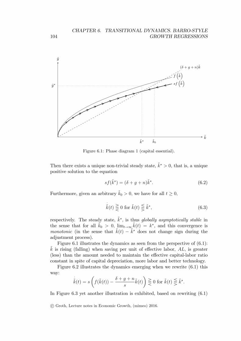
104CHAPTER 6. TRANSITIONAL DYNAMICS. BARRO-STYLE
GROWTH REGRESSIONS
k∗ k0
y∗
(δ + g + n)k
f(k)
sf(k)
k
y
Figure 6.1: Phase diagram 1 (capital essential).
Then there exists a unique non-trivial steady state, k∗ > 0, that is, a uniquepositive solution to the equation
sf(k∗) = (δ + g + n)k∗. (6.2)
Furthermore, given an arbitrary k0 > 0, we have for all t ≥ 0,
·k(t) T 0 for k(t) S k∗, (6.3)
respectively. The steady state, k∗, is thus globally asymptotically stable inthe sense that for all k0 > 0, limt→∞ k(t) = k∗, and this convergence ismonotonic (in the sense that k(t) − k∗ does not change sign during theadjustment process).Figure 6.1 illustrates the dynamics as seen from the perspective of (6.1):
k is rising (falling) when saving per unit of effective labor, AL, is greater(less) than the amount needed to maintain the effective capital-labor ratioconstant in spite of capital depreciation, more labor and better technology.Figure 6.2 illustrates the dynamics emerging when we rewrite (6.1) this
way:·k(t) = s
(f(k(t))− δ + g + n
sk(t)
)T 0 for k(t) S k∗.
In Figure 6.3 yet another illustration is exhibited, based on rewriting (6.1)
c© Groth, Lecture notes in Economic Growth, (mimeo) 2016.

6.1. Point of departure: the Solow model 105
k∗ k0
y∗
(δ + g + n)
sk
f(k)
k
y
Figure 6.2: Phase diagram 2.
k0 k∗
δ + g + n
sf(k)
k
gk
k
SK
Figure 6.3: Phase diagram 3.
c© Groth, Lecture notes in Economic Growth, (mimeo) 2016.

106CHAPTER 6. TRANSITIONAL DYNAMICS. BARRO-STYLE
GROWTH REGRESSIONS
this way:·k(t)
k(t)= s
f(k(t))
k(t)− (δ + g + n),
where sf(k(t))/k(t) is gross saving per unit of capital, S(t)/K(t) ≡ (Y (t)−C(t))/K(t).From now on the dating of the variables is suppressed unless needed for
clarity.
6.2 Do poor countries tend to approach theirsteady state from below?
From some textbooks (for instance Barro and Sala-i-Martin, 2004) one getsthe impression that poor countries tend to approach their steady state frombelow. But this is not what the Penn World Table data seems to indicate.And from a theoretical point of view the size of k0 relative to k∗ is certainlyambiguous, whether the country is rich or poor. To see this, consider a poorcountry with initial effective capital intensity
k0 ≡K0
A0L0
.
Here K0/L0 will typically be small for a poor country (the country has notyet accumulated much capital relative to its fast-growing population). Thetechnology level, A0, however, also tends to be small for a poor country.Hence, whether we should expect k0 < k∗ or k0 > k∗ is not obvious apriori.Or equivalently: whether we should expect that a poor country’s GDP at anarbitrary point in time grows at a rate higher or lower than the country’ssteady-state growth rate, g + n, is not obvious apriori.While Figure 6.3 illustrates the case where the inequality k0 < k∗ holds,
Figure 6.1 and 6.2 illustrate the opposite case. There exists some empiricalevidence indicating that poor countries tend to approach their steady statefrom above. Indeed, Cho and Graham (1996) find that “on average, countrieswith a lower income per adult are above their steady-state positions, whilecountries with a higher income are below their steady-state positions”.The prejudice that poor countries apriori should tend to approach their
steady state from below seems to come from a confusion of conditional andunconditional β convergence. The Solow model predicts - and data supports- that within a group of countries with similar structural characteristics (ap-proximately the same f, A0, g, s, n, and δ), the initially poorer countries will
c© Groth, Lecture notes in Economic Growth, (mimeo) 2016.

6.3. Within-country convergence speed and adjustment time 107
grow faster than the richer countries. This is because the poorer countries(small y(0) = f(k0)A0) will be the countries with relatively small initialcapital-labor ratio, k0. As all the countries in the group have approximatelythe same A0, the poorer countries thus have k0 ≡ k0/A0 relatively small, i.e.,k0 < k∗. From y ≡ Y/L ≡ yA = f(k)A follows that the growth rate inoutput per worker of these poor countries tends to exceed g. Indeed, we havegenerally (for instance in the Solow model as well as the Ramsey model)
y
y=
·y
y+ g =
f ′(k)·k
f(k)+ g T g for
·k T 0, i.e., for k S k∗.
So, within the group, the poor countries tend to approach the steady state,k∗, from below.The countries in the world as a whole, however, differ a lot w.r.t. their
structural characteristics, including their A0. Unconditional β convergence isdefinitely rejected by the data. Then there is no reason to expect the poorercountries to have k0 < k∗ rather than k0 > k∗. Indeed, according to thementioned study by Cho and Graham (1996), it turns out that the data forthe relatively poor countries favors the latter inequality rather than the first.
6.3 Within-country convergence speed and ad-justment time
Our next issue is: How fast (or rather how slow) are the transitional dynamicsin a growth model? To put it another way: according to a given growth modelwith convergence, how fast does the economy approach its steady state? Theanswer turns out to be: not very fast - to say the least. This is a rathergeneral conclusion and is confirmed by the empirics: adjustment processesin a growth context are quite time consuming.In Acemoglu (2009) we meet the concept of speed of convergence at p.
54 (under an alternative name, rate of adjustment) and p. 81 (in connectionwith Barro-style growth regressions). Here we shall go more into detail withthe issue of speed of convergence.Again the Solow model is our frame of reference. We search for a formula
for the speed of convergence of k(t) and y(t)/y∗(t) in a closed economy de-scribed by the Solow model. So our analysis is concerned with within-countryconvergence: how fast do variables such as k and y approach their steadystate paths in a closed economy? The key adjustment mechanism is linkedto diminishing returns to capital (falling marginal productivity of capital)
c© Groth, Lecture notes in Economic Growth, (mimeo) 2016.

108CHAPTER 6. TRANSITIONAL DYNAMICS. BARRO-STYLE
GROWTH REGRESSIONS
in the process of capital accumulation. The problem of cross-country con-vergence (which is what “β convergence” and “σ convergence” are about)is in principle more complex because also such mechanisms as technologicalcatching-up and cross-country factor movements are involved.
6.3.1 Convergence speed for k(t)
The ratio of·k(t) to (k(t)− k∗) 6= 0 can be written
·k(t)
k(t)− k∗=d(k(t)− k∗)/dt
k(t)− k∗, (6.4)
since dk∗/dt = 0. We define the instantaneous speed of convergence at time
t as the (proportionate) rate of decline of the distance∣∣∣k(t)− k∗
∣∣∣ at time tand we denote it SOCt(k).1 Thus,
SOCt(k) ≡ −d(∣∣∣k(t)− k∗
∣∣∣) /dt∣∣∣k(t)− k∗∣∣∣ = −d(k(t)− k∗)/dt
k(t)− k∗(6.5)
per time unit, where the equality sign is valid for monotonic convergence.Generally, SOCt(k) depends on both the absolute size of the difference k
− k∗ at time t and its sign. But if the difference is already “small”, SOCt(k)will be “almost”constant for increasing t and we can find an approximate
measure for it. Let the function ϕ(k) be defined by·k = sf(k)−mk ≡ ϕ(k),
where m ≡ δ+ g+n. A first-order Taylor approximation of ϕ(k) around k =k∗ gives
ϕ(k) ≈ ϕ(k∗) + ϕ′(k∗)(k − k∗) = 0 + (sf ′(k∗)−m)(k − k∗).
For k in a small neighborhood of the steady state, k∗, we thus have·k = ϕ(k) ≈ (sf ′(k∗)−m)(k − k∗)
= (sf ′(k∗)
m− 1)m(k − k∗)
= (k∗f
′(k∗)
f(k∗)− 1)m(k − k∗) (from (6.2))
≡ (ε(k∗)− 1)m(k − k∗) (from (6.6)),
1Synonyms for speed of convergence are rate of convergence, rate of adjustment oradjustment speed.
c© Groth, Lecture notes in Economic Growth, (mimeo) 2016.

6.3. Within-country convergence speed and adjustment time 109
where ε(k∗) is the output elasticity w.r.t. capital, evaluated in the steadystate. So
K
Y
∂Y
∂K=
k
f(k)f ′(k) ≡ ε(k), (6.6)
where 0 < ε(k) < 1 for all k > 0.
Applying the definition (6.5) and the identity m ≡ δ+ g+ n, we now get
SOCt(k) = −d(k(t)− k∗)/dtk(t)− k∗
=−·k(t)
k(t)− k∗≈ (1−ε(k∗))(δ+g+n) ≡ β(k∗) > 0.
(6.7)This result tells us how fast, approximately, the economy approaches itssteady state if it starts “close”to it. If, for example, β(k∗) = 0.02 per year,then 2 percent of the gap between k(t) and k∗ vanishes per year. We also seethat everything else equal, a higher output elasticity w.r.t. capital implies alower speed of convergence.
In the limit, for∣∣∣k − k∗∣∣∣ → 0, the instantaneous speed of convergence
coincides with what is called the asymptotic speed of convergence, defined as
SOC∗(k) ≡ lim|k−k∗|→0
SOCt(k) = β(k∗). (6.8)
Multiplying through by −(k(t)− k∗), the equation (6.7) takes the form ofa homogeneous linear differential equation (with constant coeffi cient), x(t) =βx(t), the solution of which is x(t) = x(0)eβt.With x(t) = k(t)− k∗ and “=”replaced by “≈”, we get in the present case
k(t)− k∗ ≈ (k(0)− k∗)e−β(k∗)t → 0 for t→∞. (6.9)
This is the approximative time path for the gap between k(t) and k∗ andshows how the gap becomes smaller and smaller at the rate β(k∗).One of the reasons that the speed of convergence is important is that it
indicates what weight should be placed on transitional dynamics of a growthmodel relative to the steady-state behavior. The speed of convergence mat-ters for instance for the evaluation of growth-promoting policies. In growthmodels with diminishing marginal productivity of production factors, suc-cessful growth-promoting policies have transitory growth effects and perma-nent level effects. Slower convergence implies that the full benefits are slowerto arrive.
c© Groth, Lecture notes in Economic Growth, (mimeo) 2016.

110CHAPTER 6. TRANSITIONAL DYNAMICS. BARRO-STYLE
GROWTH REGRESSIONS
6.3.2 Convergence speed for log k(t)*
We have found an approximate expression for the convergence speed of k.Since models in empirical analysis and applied theory are often based on log-linearization, we might ask what the speed of convergence of log k is. Theanswer is: approximately the same and asymptotically exactly the same asthat of k itself! Let us see why.A first-order Taylor approximation of log k(t) around k = k∗ gives
log k(t) ≈ log k∗ +1
k∗(k(t)− k∗). (6.10)
By definition
SOCt(log k) = −d(log k(t)− log k∗)/dt
log k(t)− log k∗= − dk(t)/dt
k(t)(log k(t)− log k∗)
≈ − dk(t)/dt
k(t) k(t)−k∗k∗
=k∗
k(t)SOCt(k)→ SOC∗(k) = β(k∗)(6.11)
for k(t) → k∗,
where in the second line we have used, first, the approximation (6.10), second,the definition in (6.7), and third, the definition in (6.8).So, at least in a neighborhood of the steady state, the instantaneous rate
of decline of the logarithmic distance of k to the steady-state value of kapproximates the instantaneous rate of decline of the distance of k itself toits steady-state value. The asymptotic speed of convergence of log k coincideswith that of k itself and is exactly β(k∗).In the Cobb-Douglas case (where ε(k∗) is a constant, say α) it is possible
to find an explicit solution to the Solow model, see Acemoglu (2009, p. 53)and Exercise II.2. It turns out that the instantaneous speed of convergence ina finite distance from the steady state is a constant and equals the asymptoticspeed of convergence, (1− α)(δ + g + n).
6.3.3 Convergence speed for y(t)/y∗(t)*
The variable which we are interested in is usually not so much k in itself,but rather labor productivity, y(t) ≡ y(t)A(t). In the interesting case whereg > 0, labor productivity does not converge towards a constant. We thereforefocus on the ratio y(t)/y∗(t), where y∗(t) denotes the hypothetical value oflabor productivity at time t, conditional on the economy being on its steady-state path, i.e.,
y∗(t) ≡ y∗A(t). (6.12)
c© Groth, Lecture notes in Economic Growth, (mimeo) 2016.

6.3. Within-country convergence speed and adjustment time 111
We havey(t)
y∗(t)≡ y(t)A(t)
y∗A(t)=y(t)
y∗. (6.13)
As y(t)→ y∗ for t→∞, the ratio y(t)/y∗(t) converges towards 1 for t→∞.Taking logs on both sides of (6.13), we get
logy(t)
y∗(t)= log
y(t)
y∗= log y(t)− log y∗
≈ log y∗ +1
y∗(y(t)− y∗)− log y∗ (first-order Taylor approx. of log y )
=1
f(k∗)(f(k(t))− f(k∗))
≈ 1
f(k∗)(f(k∗) + f ′(k∗)(k(t)− k∗)− f(k∗)) (first-order approx. of f(k))
=k∗f ′(k∗)
f(k∗)
k(t)− k∗
k∗≡ ε(k∗)
k(t)− k∗
k∗
≈ ε(k∗)(log k(t)− log k∗) (by (6.10)). (6.14)
Multiplying through by −(log k(t)− log k∗) in (6.11) and carrying out thedifferentiation w.r.t. time, we find an approximate expression for the growthrate of k,
dk(t)/dt
k(t)≡ gk(t) ≈ −
k∗
k(t)SOCt(k)(log k(t)− log k∗)
→ −β(k∗)(log k(t)− log k∗) for k(t)→ k∗, (6.15)
where the convergence follows from the last part of (6.11). We now calculatethe time derivative on both sides of (6.14) to get
d(logy(t)
y∗(t))/dt = d(log
y(t)
y∗)/dt =
dy(t)/dt
y(t)≡ gy(t)
≈ ε(k∗)gk(t) ≈ −ε(k∗)β(k∗)(log k(t)− log k∗). (6.16)
from (6.15). Dividing through by − log(y(t)/y∗(t)) in this expression, taking(6.14) into account, gives
−d(log y(t)
y∗(t))/dt
log y(t)y∗(t)
= −d(log y(t)
y∗(t) − log 1)/dt
log y(t)y∗(t) − log 1
≡ SOCt(logy
y∗) ≈ β(k∗), (6.17)
in view of log 1 = 0. So the logarithmic distance of y from its value on thesteady-state path at time t has approximately the same rate of decline as the
c© Groth, Lecture notes in Economic Growth, (mimeo) 2016.

112CHAPTER 6. TRANSITIONAL DYNAMICS. BARRO-STYLE
GROWTH REGRESSIONS
logarithmic distance of k from k’s value on the steady-state path at time t.The asymptotic speed of convergence for log y(t)/y∗(t) is exactly the sameas that for k, namely β(k∗).What about the speed of convergence of y(t)/y∗(t) itself? Here the same
principle as in (6.11) applies. The asymptotic speed of convergence forlog(y(t)/y∗(t)) is the same as that for y(t)/y∗(t) (and vice versa), namelyβ(k∗).With one year as our time unit, standard parameter values are: g = 0.02,
n = 0.01, δ = 0.05, and ε(k∗) = 1/3.We then get β(k∗) = (1−ε(k∗))(δ+g+n)= 0.053 per year. In the empirical Chapter 11 of Barro and Sala-i-Martin(2004), it is argued that a lower value of β(k∗), say 0.02 per year, fits the databetter. This requires ε(k∗) = 0.75. Such a high value of ε(k∗) (≈ the incomeshare of capital) may seem diffi cult to defend. But if we reinterpret K inthe Solow model so as to include human capital (skills embodied in humanbeings and acquired through education and learning by doing), a value ofε(k∗) at that level may not be far out.
6.3.4 Adjustment time
Let τω be the time that it takes for the fraction ω ∈ (0, 1) of the initial gapbetween k and k∗ to be eliminated, i.e., τω satisfies the equation∣∣∣k(τω)− k∗
∣∣∣∣∣∣k(0)− k∗∣∣∣ =
k(τω)− k∗
k(0)− k∗= 1− ω, (6.18)
where 1 − ω is the fraction of the initial gap still remaining at time τω. In(6.18) we have applied that sign(k(t) − k∗) = sign(k(0) − k∗) in view ofmonotonic convergence.By (6.9), we have
k(τω)− k∗ ≈ (k(0)− k∗)e−β(k∗)τω .
In view of (6.18), this implies
1− ω ≈ e−β(k∗)τω .
Taking logs on both sides and solving for τω gives
τω ≈ −log(1− ω)
β(k∗). (6.19)
c© Groth, Lecture notes in Economic Growth, (mimeo) 2016.

6.3. Within-country convergence speed and adjustment time 113
This is the approximate adjustment time required for k to eliminate thefraction ω of the initial distance of k to its steady-state value, k∗, when theadjustment speed (speed of convergence) is β(k∗).Often we consider the half-life of the adjustment, that is, the time it
takes for half of the initial gap to be eliminated. To find the half-life of theadjustment of k, we put ω = 1
2in (6.19). Again we use one year as our time
unit. With the parameter values from Section 6.3.3, we have β(k∗) = 0.053per year and thus
τ 12≈ −
log 12
0.053≈ 0.69
0.053= 13, 1 years.
As noted above, Barro and Sala-i-Martin (2004) estimate the asymptoticspeed of convergence to be β(k∗) = 0.02 per year. With this value, thehalf-life is approximately
τ 12≈ −
log 12
0.02≈ 0.69
0.02= 34.7 years.
And the time needed to eliminate three quarters of the initial distance tosteady state, τ 3/4, will then be about 70 years (= 2 ·35 years, since 1−3/4 =12· 1
2).Among empirical analysts there is not general agreement about the size of
β(k∗). Some authors, for example Islam (1995), using a panel data approach,find speeds of convergence considerably larger, between 0.05 and 0.09. Mc-Quinne and Whelan (2007) get similar results. There is a growing realizationthat the speed of convergence differs across periods and groups of countries.Perhaps an empirically reasonable range is 0.02 < β(k∗) < 0.09. Correspond-ingly, a reasonable range for the half-life of the adjustment will be 7.6 years< τ 1
2< 34.7 years.
Most of the empirical studies of convergence use a variety of cross-countryregression analysis of the kind described in the next section. Yet the theoret-ical frame of reference is often the Solow model - or its extension with humancapital (Mankiw et al., 1992). These models are closed economy models withexogenous technical progress and deal with “within-country”convergence. Itis not obvious that they constitute an appropriate framework for studyingcross-country convergence in a globalized world where capital mobility and tosome extent also labor mobility are important and where some countries arepushing the technological frontier further out, while others try to imitate andcatch up. At least one should be aware that the empirical estimates obtainedmay reflect mechanisms in addition to the falling marginal productivity ofcapital in the process of capital accumulation.
c© Groth, Lecture notes in Economic Growth, (mimeo) 2016.

114CHAPTER 6. TRANSITIONAL DYNAMICS. BARRO-STYLE
GROWTH REGRESSIONS
6.4 Barro-style growth regressions*
Barro-style growth regression analysis, which became very popular in the1990s, draws upon transitional dynamics aspects (including the speed of con-vergence) as well as steady state aspects of neoclassical growth theory (forinstance the Solow model or the Ramsey model).Chapter 3.2 in Acemoglu (2009) presents Barro’s growth regression equa-
tions in an unconventional form, see Acemoglu’s equations (3.12), (3.13), and(3.14). The left-hand side appears as if it is just the growth rate of y (outputper unit of labor) from one year to the next. But the true left-hand side of aBarro equation is the average compound annual growth rate of y over manyyears. Moreover, since Acemoglu’s text is very brief about the formal linksto the underlying neoclassical theory of transitional dynamics, we will spellthe details out here.Most of the preparatory work has already been done above. The point of
departure is a neoclassical one-sector growth model for a closed economy:
·k(t) = s(k(t))f(k(t))− (δ + g + n)k(t), k(0) = k0 > 0, given, (6.20)
where k(t) ≡ K(t)/(A(t)L(t)), A(t) = A0egt, and L(t) = L0e
nt as above.The Solow model is the special case where the saving-income ratio, s(k(t)),is a constant s ∈ (0, 1).It is assumed that the model, (6.20), generates monotonic convergence,
i.e., k(t) → k∗ > 0 for t → ∞. Applying again a first-order Taylor approxi-mation, as in Section 3.1, and taking into account that s(k) now may dependon k, as for instance it generally does in the Ramsey model, we find theasymptotic speed of convergence for k to be
SOC∗(k) = (1− ε(k∗)− η(k∗))(δ + g + n) ≡ β(k∗) > 0, (*)
where η(k∗) ≡ k∗s′(k∗)/s(k∗) is the elasticity of the saving-income ratio w.r.t.the effective capital intensity, evaluated at k = k∗. (In case of the Ramseymodel, one can alternatively use the fact that SOC∗(k) equals the absolutevalue of the negative eigenvalue of the Jacobian matrix associated with thedynamic system of the model, evaluated in the steady state. For a fullyspecified Ramsey model this eigenvalue can be numerically calculated by anappropriate computer algorithm; in the Cobb-Douglas case there exists evenan explicit algebraic formula for the eigenvalue, see Barro and Sala-i-Martin,2004). In a neighborhood of the steady state, the previous formulas remainvalid with β(k∗) defined as in (*). The asymptotic speed of convergence of forexample y(t)/y∗(t) is thus β(k∗) as given in (*). For notational convenience,
c© Groth, Lecture notes in Economic Growth, (mimeo) 2016.
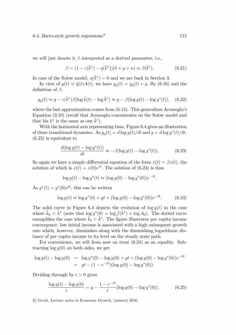
6.4. Barro-style growth regressions* 115
we will just denote it β, interpreted as a derived parameter, i.e.,
β = (1− ε(k∗)− η(k∗))(δ + g + n) ≡ β(k∗). (6.21)
In case of the Solow model, η(k∗) = 0 and we are back in Section 3.In view of y(t) ≡ y(t)A(t), we have gy(t) = gy(t) + g. By (6.16) and the
definition of β,
gy(t) ≈ g − ε(k∗)β(log k(t)− log k∗) ≈ g − β(log y(t)− log y∗(t)), (6.22)
where the last approximation comes from (6.14). This generalizes Acemoglu’sEquation (3.10) (recall that Acemoglu concentrates on the Solow model andthat his k∗ is the same as our k∗).With the horizontal axis representing time, Figure 6.4 gives an illustration
of these transitional dynamics. As gy(t) = d log y(t)/dt and g = d log y∗(t)/dt,(6.22) is equivalent to
d(log y(t)− log y∗(t))
dt≈ −β(log y(t)− log y∗(t)). (6.23)
So again we have a simple differential equation of the form x(t) = βx(t), thesolution of which is x(t) = x(0)eβt. The solution of (6.23) is thus
log y(t)− log y∗(t) ≈ (log y(0)− log y∗(0))e−βt.
As y∗(t) = y∗(0)egt, this can be written
log y(t) ≈ log y∗(0) + gt+ (log y(0)− log y∗(0))e−βt. (6.24)
The solid curve in Figure 6.4 depicts the evolution of log y(t) in the casewhere k0 < k∗ (note that log y∗(0) = log f(k∗) + logA0). The dotted curveexemplifies the case where k0 > k∗. The figure illustrates per capita incomeconvergence: low initial income is associated with a high subsequent growthrate which, however, diminishes along with the diminishing logarithmic dis-tance of per capita income to its level on the steady state path.For convenience, we will from now on treat (6.24) as an equality. Sub-
tracting log y(0) on both sides, we get
log y(t)− log y(0) = log y∗(0)− log y(0) + gt+ (log y(0)− log y∗(0))e−βt
= gt− (1− e−βt)(log y(0)− log y∗(0)).
Dividing through by t > 0 gives
log y(t)− log y(0)
t= g − 1− e−βt
t(log y(0)− log y∗(0)). (6.25)
c© Groth, Lecture notes in Economic Growth, (mimeo) 2016.

116CHAPTER 6. TRANSITIONAL DYNAMICS. BARRO-STYLE
GROWTH REGRESSIONS
0 0log log ( )A f k
0
log ( )y t
0log log ( *)A f k g
t
log *( )y t
Figure 6.4: Evolution of log y(t). Solid curve: the case k0 < k∗. Dotted curve: thecase k0 > k∗. Stippled line: the steady-state path.
On the left-hand side appears the average compound annual growth rate ofy from period 0 to period t, which we will denote gy(0, t). On the right-handside appears the initial distance of log y to its hypothetical level along thesteady state path. The coeffi cient, −(1− e−βt)/t, to this distance is negativeand approaches zero for t → ∞. Thus (6.25) is a translation into growthform of the convergence of log yt towards the steady-state path, log y∗t , in thetheoretical model without shocks. Rearranging the right-hand side, we get
gy(0, t) = g +1− e−βt
tlog y∗(0)− 1− e−βt
tlog y(0) ≡ b0 + b1 log y(0),
where both the constant b0 ≡ g +[(1− e−βt)/t
]log y∗(0) and the coeffi cient
b1 ≡ −(1 − e−βt)/t are determined by “structural characteristics”. Indeed,β is determined by δ, g, n, ε(k∗), and η(k∗) through (6.21), and y∗(0) is de-termined by A0 and f(k∗) through (6.12), where, in turn, k∗ is determinedby the steady state condition s(k∗)f(k∗) = (δ + g + n)k∗, s(k∗) being thesaving-income ratio in the steady state.With data for N countries, i = 1, 2,. . . , N, a test of the unconditional
convergence hypothesis may be based on the regression equation
gyi(0, t) = b0 + b1 log yi(0) + εi, εi ∼ N(0, σ2ε), (6.26)
where εi is the error term. This can be seen as a Barro growth regressionequation in its simplest form. For countries in the entire world, the theoret-
c© Groth, Lecture notes in Economic Growth, (mimeo) 2016.

6.4. Barro-style growth regressions* 117
ical hypothesis b1 < 0 is clearly not supported (or, to use the language ofstatistics, the null hypothesis, b1 = 0, is not rejected).2
Allowing for the considered countries having different structural charac-teristics, the Barro growth regression equation takes the form
gyi(0, t) = b0i + b1 log yi(0) + εi, b1 < 0, εi ∼ N(0, σ2
ε). (6.27)
In this “fixed effects” form, the equation has been applied for a test of theconditional convergence hypothesis, b1 < 0, often supporting this hypothesis.That is, within groups of countries with similar characteristics (like, e.g., theOECD countries), there is a tendency to convergence.From the estimate of b1 the implied estimate of the asymptotic speed of
convergence, β, is readily obtained through the formula b1 ≡ (1 − e−βt)/t.Even β, and therefore also the slope, b1, does depend, theoretically, oncountry-specific structural characteristics. But the sensitivity on these donot generally seem large enough to blur the analysis based on (6.27) whichabstracts from this dependency.With the aim of testing hypotheses about growth determinants, Barro
(1991) and Barro and Sala-i-Martin (1992, 2004) decompose b0i so as to reflect
the role of a set of potentially causal measurable variables,
b0i = α0 + α1xi1 + α2xi2 + . . . + αmxim,
where the α’s are the coeffi cients and the x’s are the potentially causal vari-ables.3 These variables could be measurable Solow-type parameters amongthose appearing in (6.20) or a broader set of determinants, including for in-stance the educational level in the labor force, and institutional variables likerule of law and democracy. Some studies include the initial within-countryinequality in income or wealth among the x’s and extend the theoreticalframework correspondingly.4
From an econometric point of view there are several problematic featuresin regressions of Barro’s form (also called the β convergence approach). Theseproblems are discussed in Acemoglu pp. 82-85.
2Cf. Acemoglu, p. 16. For the OECD countries, however, b1 is definitely found to benegative (cf. Acemoglu, p. 17).
3Note that our α vector is called β in Acemoglu, pp. 83-84. So Acemoglu’s β is to bedistinquished from our β which denotes the asymptotic speed of convergence.
4See, e.g., Alesina and Rodrik (1994) and Perotti (1996), who argue for a negativerelationship between inequality and growth. Forbes (2000), however, rejects that thereshould be a robust negative correlation between the two.
c© Groth, Lecture notes in Economic Growth, (mimeo) 2016.

118CHAPTER 6. TRANSITIONAL DYNAMICS. BARRO-STYLE
GROWTH REGRESSIONS
6.5 References
Alesina, A., and D. Rodrik, 1994, Distributive politics and economic growth,Quarterly Journal of Economics, vol. 109, 465-490.
Barro, R. J., 1991, Economic growth in a cross section of countries, Quar-terly Journal of Economics, vol. 106, 407-443.
Barro, R. J., X. Sala-i-Martin, 1992, Convergence, Journal of Political Econ-omy, vol. 100, 223-251.
Barro, R., and X. Sala-i-Martin, 2004, Economic Growth. Second edition,MIT Press: Cambridge (Mass.).
Cho, D., and S. Graham, 1996, The other side of conditional convergence,Economics Letters, vol. 50, 285-290.
Forbes, K.J., 2000, A reassessment of the relationship between inequalityand growth, American Economic Review, vol. 90, no. 4, 869-87.
Groth, C., and R. Wendner, 2014, Embodied learning by investing andspeed of convergence, Journal of Macroeconomics, vol. 40, 245-269.
Islam, N., 1995, Growth Empirics. A Panel Data Approach, QuarterlyJournal of Economics, vol. 110, 1127-1170.
McQinn, K., K. Whelan, 2007, Conditional Convergence and the Dynamicsof the Capital-Output Ratio, Journal of Economic Growth, vol. 12,159-184.
Perotti, R., 1996, Growth, income distribution, and democracy: What thedata say, Journal of Economic Growth, vol. 1, 149-188.
c© Groth, Lecture notes in Economic Growth, (mimeo) 2016.

Chapter 7
Why the Malthusian era mustcome to an end
This chapter presents the population-breeds-ideas model by Michael Kremer(Kremer, 1993). The point of the model is to show that under certain con-ditions, the cumulative and nonrival character of technical knowledge makesit almost inevitable that the Malthusian regime of stagnating income percapita, close to subsistence minimum, will sooner or later in the historicalevolution be surpassed.This topic relates to Section 8.2 of Jones and Vollrath (2013). Section 4.2
of Acemoglu (2009) briefly discuss two special cases of the Kremer model.
7.1 The general model
Suppose a pre-industrial economy can be described by:
Yt = Aσt Lαt Z
1−α, σ > 0, 0 < α < 1, (7.1)
At = λAεtLt, λ > 0, A0 > 0 given, (7.2)
Lt =Yty, y > 0, (7.3)
where Y is aggregate output, A the level of technical knowledge, L the laborforce (= population), Z the amount of land (fixed), and y subsistence mini-mum. By this is not meant some point almost at starvation, but an incomelevel suffi cient for food, clothing, shelter etc. to the worker, including familyand offspring, thereby enabling reproduction of the labor force.Both Z and y are considered as constant parameters. Time is continuous
and it is understood that a kind of Malthusian population mechanism (seebelow) is operative behind the scene.
119

120CHAPTER 7. MICHAEL KREMER’S
POPULATION-BREEDS-IDEAS MODEL
The exclusion of capital from the aggregate production function, (7.1),reflects the presumption that capital (tools etc.) is quantitatively of minorimportance in a pre-industrial economy. In accordance with the replicationargument, the production function has CRS w.r.t. the rival inputs, labor andland. The factor Aσt measures total factor productivity. As the right-handside of (7.2) is positive, the technology level, At, is rising over time (althoughfar back in time very very slowly). The increase in At per time unit is seento be an increasing function of the size of the population. This reflects thehypothesis that population breeds ideas; these are nonrival and enter thepool of technical knowledge available for society as a whole. Indeed, theuse of an idea by one agent does not preclude others’use of the same idea.Dividing through by L in (7.1) we see that y ≡ Yt/Lt = Aσt (Z/Lt)
1−α. Thenonrival character is displayed by labor productivity being dependent on thetotal stock of knowledge, not on this stock per worker. In contrast, laborproductivity depends on land per worker.The rate per capita by which population breeds ideas is λAε. In case ε > 0,
this rate is an increasing function of the already existing level of technicalknowledge. This case reflects the hypothesis that the larger is the stock ofideas the easier do new ideas arise (perhaps by combination of existing ideas).The opposite case, ε < 0, is the one where “the easiest ideas are found first”or “the low-hanging fruits are picked first”.Equation (7.3) is a shortcut description of a Malthusian population mech-
anism. Suppose the true mechanism is
Lt = β(yt − y)Lt T 0 for yt T y, (7.4)
where β > 0 is the speed of adjustment, yt is per capita income, and y >0 is subsistence minimum. A rise in yt above y will lead to increases inLt through earlier marriage, higher fertility, and lower mortality. Therebydownward pressure on Yt/Lt is generated, perhaps pushing yt below y.Whenthis happens, population will be decreasing for a while and so return towardsits sustainable level, Yt/y. Equation (7.3) treats this mechanism as if thepopulation instantaneously adjusts to its sustainable level (i.e., as if β →∞).The model hereby gives a long-run picture, ignoring the Malthusian ups anddowns in population and per capita income about the subsistence minimum.The important feature is that the technology level, and thereby Yt, as wellas the sustainable population will be rising over time. This speeds up thearrival of new ideas and so Yt is raised even faster although per-capita incomeremains at its long-run level, y.1
For simplicity, we now normalize the constant Z to be 1.1Extending the model with the institution of private ownership and competitive mar-
kets, the absence of a growing standard of living corresponds to the doctrine from classical
c© Groth, Lecture notes in Economic Growth, (mimeo) 2016.

7.2. Law of motion 121
7.2 Law of motion
The dynamics of the model can be reduced to one differential equation, thelaw of motion of technical knowledge. By (7.3) and (7.1), Lt = Yt/y =Aσt L
αt /y. Consequently L
1−αt = Aσt /y so that
Lt = y1
α−1Aσ
1−αt . (7.5)
Substituting this into (7.2) gives the law of motion of technical knowledge:
At = λy1
α−1Aε+ σ
1−αt ≡ λAµt , (7.6)
where we have defined λ ≡ λy1/(α−1) and µ ≡ ε + σ/(1− α). As will appearin the remainder, the “feedback parameter”µ is of key importance for thedynamics. We immediately see that if µ = 1, the differential equation (7.6)is linear, while otherwise it is nonlinear.The case µ = 1 :When µ = 1, there will be a constant growth rate gA = λ
in technical knowledge. By (7.5), this results in a constant population growthrate gL = [σ/(1− α)] λ, which is also the growth rate of output in view of(7.3). By the definition of λ in (7.6), we see that, as expected, the populationand output growth rate is an increasing function of the creativity parameterλ and a decreasing function of the subsistence minimum.2
In this case the economy never leaves the Malthusian regime of a more orless constant standard of living close to existence minimum. Takeoff neveroccurs.The case µ 6= 1. Then (7.6) can be written
At = λAµt , (7.7)
which is a nonlinear differential equation in A.3 Let x ≡ A1−µ. Then
xt = (1− µ)A−µt λAµt = (1− µ)λ, (7.8)
economics called the iron law of wages. This is the theory (from Malthus and Ricardo)that scarce natural resources and the pressure from population growth causes real wagesto remain at subsistende level. There may occationally occur a technological improvement,which leads to a transitory real wage increase, triggering of an increase in population whichultimately brings down wages.These classical economists did not recognize any tendency to sustained technical progress
and therefore missed the immanent tendency to sustained population growth at the pre-industrial stage of economic development. Karl Marx was the first among the classicaleconomists to really see and emphasize sustained technical progress.
2If σ = 1 − α as in Acemoglu’s analysis, µ = 1 requires ε = 0, and in this case L andY grow at the same rate as knowledge.
3The differential equation, (7.7), is a special case of what is known as the Bernoulliequation. In spite of being a non-linear differential equation, the Bernoulli equation alwayshas an explicit solution.
c© Groth, Lecture notes in Economic Growth, (mimeo) 2016.

122CHAPTER 7. MICHAEL KREMER’S
POPULATION-BREEDS-IDEAS MODEL
a constant. To find xt from this, we only need simple integration:
xt = x0 +
∫ t
0
xτdτ = x0 + (1− µ)λt.
As A = x1
1−µ and x0 = A1−µ0 , this implies
At = x1
1−µt =
[A1−µ
0 + (1− µ)λt] 11−µ
=1[
A1−µ0 − (µ− 1)λt
] 1µ−1
. (7.9)
There are now two sub-cases, µ > 1 and µ < 1. The latter sub-case leadsto permanent but decelerating growth in knowledge and population and theMalthusian regime is never transcended (see Exercise III.3). The formersub-case is the interesting one.
7.3 The inevitable ending of the Malthusianregime when µ > 1
Assume µ > 1. In this case the result (7.9) implies that the Malthusianregime must come to an end.Although to begin with, At may grow extremely slowly, the growth in At
will be accelerating because of the positive feedback (visible in (7.2)) fromboth rising population and rising At. Indeed, since µ > 1, the denominatorin (7.9) will be decreasing over time and approach zero in finite time, namelyas t approaches the finite value t∗ = A1−µ
0 /((µ − 1)λ). As an implication,according to (7.9), At goes towards infinity in finite time. The stylizedgraph in Fig. 7.1 illustrates. The evolution of technical knowledge becomesexplosive as t approaches t∗.It follows from (7.5) and (7.1) that explosive growth in A implies explosive
growth in L and Y, respectively. The acceleration in the evolution of Y willsooner or later make Y rise fast enough so that the Malthusian populationmechanism (which for biological reasons has to be slow) can not catch up.Then, what was in the Malthusian regime only a transitory excess of yt overy, will at some t = t < t∗ become a permanent excess and take the form ofsustained growth in yt.We may think of this post-Malthusian phase as describing pre-industrial
Britain. Technological innovations speeded up, helped by market-friendlyinstitutions, intellectual property rights, and deliberate and systematic ap-plication of science and engineering. This lead to the takeoff known as theindustrial revolution.
c© Groth, Lecture notes in Economic Growth, (mimeo) 2016.
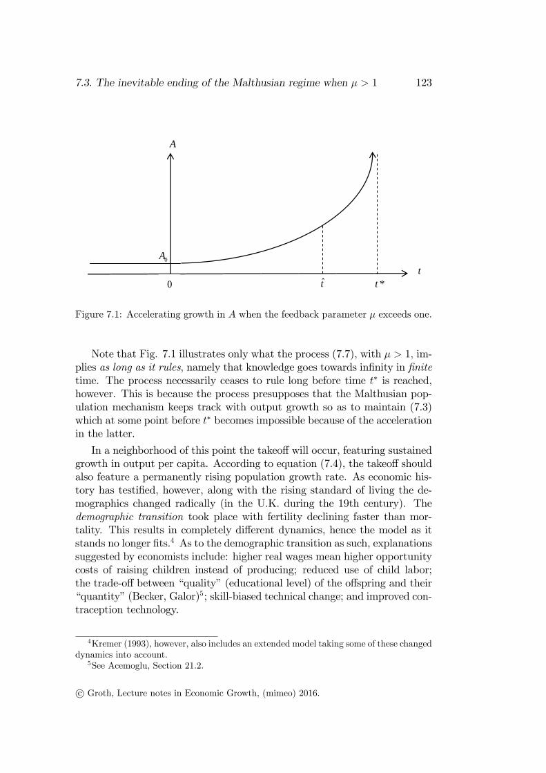
7.3. The inevitable ending of the Malthusian regime when µ > 1 123
*t
0A
t
A
0
t
Figure 7.1: Accelerating growth in A when the feedback parameter µ exceeds one.
Note that Fig. 7.1 illustrates only what the process (7.7), with µ > 1, im-plies as long as it rules, namely that knowledge goes towards infinity in finitetime. The process necessarily ceases to rule long before time t∗ is reached,however. This is because the process presupposes that the Malthusian pop-ulation mechanism keeps track with output growth so as to maintain (7.3)which at some point before t∗ becomes impossible because of the accelerationin the latter.
In a neighborhood of this point the takeoffwill occur, featuring sustainedgrowth in output per capita. According to equation (7.4), the takeoff shouldalso feature a permanently rising population growth rate. As economic his-tory has testified, however, along with the rising standard of living the de-mographics changed radically (in the U.K. during the 19th century). Thedemographic transition took place with fertility declining faster than mor-tality. This results in completely different dynamics, hence the model as itstands no longer fits.4 As to the demographic transition as such, explanationssuggested by economists include: higher real wages mean higher opportunitycosts of raising children instead of producing; reduced use of child labor;the trade-off between “quality”(educational level) of the offspring and their“quantity”(Becker, Galor)5; skill-biased technical change; and improved con-traception technology.
4Kremer (1993), however, also includes an extended model taking some of these changeddynamics into account.
5See Acemoglu, Section 21.2.
c© Groth, Lecture notes in Economic Growth, (mimeo) 2016.
124CHAPTER 7. MICHAEL KREMER’S
POPULATION-BREEDS-IDEAS MODEL
7.4 Closing remarks
The population-breeds-ideas model is about dynamics in the Malthusianregime of the pre-industrial epoch. The story told by the model is the follow-ing. When the feedback parameter, µ, is above one, the Malthusian regimehas to come to an end because the battle between scarcity of land (or nat-ural resources more generally) and technological progress (absent naturalcatastrophes) will inevitably be won by the latter. The reason is the cumu-lative and nonrival character of technical knowledge. This nonrivalry implieseconomies of scale. Moreover, the stock of knowledge is growing endoge-nously. This knowledge growth generates output growth and, through thedemographic mechanism (7.3), growth in the stock of people, which impliesa positive feedback to the growth of knowledge and so on. On top of this,if ε > 0, knowledge growth has a direct positive feedback on itself through(7.2). When the total positive feedback is strong enough (µ > 1), it generatesan explosive process.6
On the basis of demographers’estimates of the growth in global popu-lation over most of human history, Kremer (1993) finds empirical supportfor µ > 1. Indeed, in the opposite case, µ ≤ 1, there would not have beena rising world population growth rate since one million years B.C. to theindustrial revolution. The data in Kremer (1993, p. 682) indicates that theworld population growth rate has been more or less proportional to the sizeof population until recently.
Final remark. Compared with Kremer’s version of the model, we haveallowed σ 6= 1, but at the same time introduced a simplification relative toKremer’s setup. Kremer starts from a slightly more general ideas-formationequation, namely At = λAεtL
ψt with ψ > 0, while in our (7.2) we have assumed
ψ = 1. If ψ > 1, the ideas-creating brains reinforce one another. This onlyfortifies the acceleration in knowledge creation and thereby “supports” thecase µ > 1.7 If on the other hand 0 < ψ < 1, the idea-creating brains partlyoffset one another, for instance by simultaneously coming up with more orless the same ideas (the case of “overlap”). This generalization does notchange the qualitative results. By assuming that the number of new ideasper time unit is proportional to the stock of brains, we have chosen to focuson an intermediate case in order to avoid secondary factors blurring the mainmechanism.
6In the appendix the explosion result is considered in a general mathematical context.7Kremer’s calibration suggests ψ ≈ 6/5.
c© Groth, Lecture notes in Economic Growth, (mimeo) 2016.

7.5. Appendix 125
7.5 Appendix
A. The mathematical background
Mathematically, the background for the explosion result is that the solutionto a first-order differential equation of the form x(t) = α + bx(t)c, c > 1,b 6= 0, x(0) = x0 given, is always explosive. Indeed, the solution, x = x(t),will have the property that x(t) → ±∞ for t → t∗ for some t∗ > 0 where t∗
depends on the initial conditions; and thereby the solution is defined only ona bounded time interval which depends on the initial condition.Take the differential equation x(t) = 1 + x(t)2, x(0) = 0,as an example.
As is well-known, the solution is x(t) = tan t = sin t/ cos t, defined for t ∈(−π/2, π/2).
B. Comparison with the two special cases considered in Acemoglu(2009)
At pp. 113-14 Acemoglu presents two versions of this framework, both ofwhich assume σ = 1 − α. This assumption is arbitrary; it is included as aspecial case in our formulation above. As to the other parameter relating tothe role of knowledge, ε, Acemuglu assumes ε = 0 in his first version of theframework. This leads to constant population growth but a forever stagnat-ing standard of living (Acemoglu, p. 113). In his second version, Acemogluassumes ε = 1. This leads to many centuries of slow but (weakly) acceleratingpopulation growth and then ultimately a “takeoff”with sustained rise in thestandard of living, to be followed by the “demographic transition”(outsidethe model). This latter outcome arises for a much larger set of parametervalues than ε = 1 and is therefore theoretically more robust than appears inAcemoglu’s exposition.
7.6 References
Becker, G. S., ...
Galor, O., 2011, Unified Growth Theory, Princeton University Press.
Kremer, M., 1993, Population Growth and Technological Change: One Mil-lion B.C. to 1990, Quarterly Journal of Economics, vol. 108 (3).
Møller, N. Framroze, and P. Sharp, 2014, Malthus in cointegration space:Evidence of a post-Malthusian pre-industrial England, J. of EconomicGrowth, vol. 19 (1), 105-140.
c© Groth, Lecture notes in Economic Growth, (mimeo) 2016.

126CHAPTER 7. MICHAEL KREMER’S
POPULATION-BREEDS-IDEAS MODEL
c© Groth, Lecture notes in Economic Growth, (mimeo) 2016.

Chapter 9
Human capital, learningtechnology, and the Mincerequation
We start with an overview of different approaches to the modeling of humancapital formation in macroeconomics. Next we go into detail with one ofthese approaches, the life-cycle approach. In Section 9.3 a simple model ofthe choice of schooling length is considered. Finally, Section 9.4 presents thetheory behind the empirical relationship named the Mincer equation.1 Inthis connection it is emphasized that the Mincer equation should be seen asan equilibrium relationship for relative wages at a given point in time ratherthan as a production function for human capital.
9.1 Macroeconomic approaches to human cap-ital
We define human capital as the stock of productive skills embodied in anindividual. Human capital is thus a production factor, while by human wealthis meant the present value of expected future labor income (usually after tax).Increases in the stock of human capital occurs through formal education
and on-the-job-training. By contributing to the maintenance of life and well-being, also health care is of importance for the stock of human capital andthe incentive to invest in human capital.Since human capital is embodied in individuals and can only be used one
place at a time, it is a rival and excludable good. Human capital is thus
1After Mincer (1958, 1974).
155

156CHAPTER 9. HUMAN CAPITAL, LEARNING TECHNOLOGY,
AND THE MINCER EQUATION
very different from technical knowledge. We think of technical knowledge asa list of instructions about how different inputs can be combined to producea certain output. A principle of chemical engineering is an example of a pieceof technical knowledge. In contrast to human capital, technical knowledgeis a non-rival and only partially excludable good. Competence in applyingtechnical knowledge is one of the skills that to a larger or smaller extent ispart of human capital.
9.1.1 Modelling human capital
In the macroeconomic literature there are different theoretical approaches tothe modelling of human capital. Broadly speaking we may distinguish theseapproaches along two “dimensions”: 1) What characteristics of human capi-tal are emphasized? 2) What characteristics of the decision maker investingin human capital are emphasized? Combining these two “dimensions”, weget Table 1.
Table 1. Macroeconomic approaches to the modelling of human capital.The character of human capital (hc):
The character of the Is hc treated as essentially differentdecision maker from physical capital?
No YesSolow-type rule-of-thumb households Mankiw et al. (1992)
Infinitely-lived family “dynasties” Barro&Sala-i-Martin (2004) Lucas (1988)(the representative agent approach) Dalgaard&Kreiner (2001)Finitely-lived individuals going through Ben-Porath (1967)a life cycle (the life cycle approach) Heijdra&Romp (2009)
My personal opinion is that for most issues the approach in the lower-right corner of Table 1 is preferable, that is, the approach treating humancapital as a distinct capital good in a life cycle perspective. The viewpointis:First, by being embodied in a person and being lost upon death of this
person, human capital is very different from physical capital. In addition,investment in human capital is irreversible (can not be recovered). Humancapital is also distinct in view of the limited extend to which it can be usedas a collateral, at least in non-slave societies. Financing an investment inphysical capital, a house for example, by credit is comparatively easy becausethe house can serve as a collateral. A creditor can not gain title to a person,
c© Groth, Lecture notes in Economic Growth, (mimeo) 2016.
9.1. Macroeconomic approaches to human capital 157
however. At most a creditor can gain title to a part of that person’s futureearnings in excess of a certain level required for a “normal”or “minimum”standard of living.Second, educational investment is closely related to life expectancy and
the life cycle of human beings: school - work - retirement. So a life cycle per-spective seems the natural approach. Fortunately, convenient macroeconomicframeworks incorporating life cycle aspects exist in the form of overlappinggenerations models (for example Diamond’s OLG model or Blanchard’s con-tinuous time OLG model).
9.1.2 Human capital and the effi ciency of labor
Generally we tend to think of human capital as a combination of differentskills. Macroeconomics, however, often tries (justified or not) to boil downthe notion of human capital to a one-dimensional entity. So let us imaginethat the current stock of human capital in society is measured by the one-dimensional index H. With L denoting the size of the labor force, we defineh ≡ H/L. So, h is the average stock of human capital in the labor force.Further, let the “quality” (or “effi ciency”) of this stock in production bedenoted q (under certain conditions this quality might be proxied by theaverage real wage per man-hour). Then it is reasonable to link q and h bysome increasing quality function
q = q(h), where q(0) ≥ 0, q′ > 0. (9.1)
Consider an aggregate production function, F , giving output per timeunit at time t as
Y = F (K, q(h)L, t),∂F
∂t> 0, (9.2)
where K is input of physical capital. The third argument of F is time, t,indicating that the production function is time-dependent due to technicalprogress.Generally the macroeconomic analyst would prefer a measure of human
capital such that the quality of human capital is proportional to the stockof human capital, allowing us to write q(h) = h by normalizing the factor ofproportionality to be 1. The main reason is that an expedient variable rep-resenting human capital in a model requires that the analyst can decomposethe real wage per working hour multiplicatively into two factors, the realwage per unit of human capital per working hour and the stock of humancapital, h. That is, an expedient human capital concept requires that we canwrite
w = w · h, (9.3)
c© Groth, Lecture notes in Economic Growth, (mimeo) 2016.

158CHAPTER 9. HUMAN CAPITAL, LEARNING TECHNOLOGY,
AND THE MINCER EQUATION
where w is the real wage per unit of human capital per working hour. Indeed,if we have
Y = F (K,hL, t), (9.4)
then, under perfect competition, we can write
w =∂Y
∂L= F2(K,hL, t)h = w · h.
Under disembodied Harrod-neutral technical progress, (9.4) would takethe form
Y = F (K,hL, t) = F (K,AhL) ≡ F (K,EL), (9.5)
where E ≡ A · h is the “effective”labor input. The proportionality betweenE and h will under perfect competition allow us to write
w =∂Y
∂L= F2(K,EL, t)E = wE · E = wE · A · h = w · h.
So with the introduction of the technology level, A, an additional decomposi-tion, w = wE ·A comes in, while the original decomposition in (9.3) remainsvalid.Whether or not the desired proportionality q(h) = h can be obtained
depends on how we model the formation of the “stuff” h. Empirically itturns out that treating the formation of human capital as similar to that ofphysical capital does not lead to the desired proportionality.
Treating the formation of human capital as similar to formation ofphysical capital
Consider a model where human capital is formed in a way similar to physi-cal capital. The Mankiw-Romer-Weil (1992) extension of the Solow growthmodel with human capital is a case in point. Non-consumed aggregate outputis split into one part generating additional physical capital one-to-one, whilethe other part is assumed to generate additional human capital one-to-one.Then for a closed economy in continuous time we can write:
Y = C + IK + IH ,
K = IK − δKK, δK > 0,
H = IH − δHH, δH > 0, (9.6)
where IK and IH denote gross investment in physical and human capital, re-spectively. This approach essentially assumes that human capital is producedby the same technology as consumption and investment goods.
c© Groth, Lecture notes in Economic Growth, (mimeo) 2016.

9.1. Macroeconomic approaches to human capital 159
Suppose the huge practical measurement problems concerning IH havebeen somehow overcome. Then from long time series for IH an index for Ht
can be constructed by the perpetual inventory method in a way similar to theway an index for Kt is constructed from long time series for IK . Indeed, indiscrete time, with 0 < δH < 1, we get, by backward substitution,
Ht+1 = IH,t + (1− δH)Ht = IH,t + (1− δH) [IH,t−1 + (1− δH)Ht−1]
=
T∑i=0
(1− δH)iIH,t−i + (1− δH)T+1Ht−T . (9.7)
From the time series for IH , an estimate of δH , and a rough conjecture aboutthe initial value, Ht−T , we can calculate Ht+1. The result will not be verysensitive to the conjectured value of Ht−T since for large T the last term in(9.7) becomes very small.In principle there need not be anything wrong with this approach. A
snag arises, however, if, without further notice, the approach is combinedwith an explicit or implicit postulate that q(h) is proportional to the “stuff”,h, brought into being in the way described by (9.6). The snag is that theempirical evidence does not support this when the formation of human cap-ital is modelled as in (9.6). This is an unintended by-product of the cross-country regression analysis by Mankiw, Romer, and Weil (1992), based onthe approach in equation (9.6). One of their conclusions is that the followingproduction function for a country’s GDP is an acceptable approximation:
Y = BK1/3H1/3L1/3, (9.8)
where B stands for the total factor productivity of the country and is gen-erally growing over time.2 Applying that H = hL, we can write (9.8) thisway:
Y = BK1/3(hL)1/3L1/3 = K1/3(Ah1/2L)2/3,
where A = B3/2. That is, we end up with the form Y = F (K,Aq(h)L) whereq(h) = h1/2, not q(h) = h. We should thus not expect the real wage to risein proportion to h, when h is considered as some “stuff” formed in a waysimilar to the way physical capital is formed. (A further point is that writinga production function as in (9.8), i.e., with H and L as two separate inputs,may lead to confusion. The tangible input is L, and in this L, a certain
2The way Mankiw-Romer-Weil measure IH is indirect and questionable. In addition,the way they let their measure enter the regression equation has been criticized for con-founding the effects of the human capital stock and human capital investment, cf. Gemmel(1996) and Sianesi and Van Reenen (2003). It will take us too far to go into detail withthese problems here.
c© Groth, Lecture notes in Economic Growth, (mimeo) 2016.
160CHAPTER 9. HUMAN CAPITAL, LEARNING TECHNOLOGY,
AND THE MINCER EQUATION
“normal”or average h is embodied. In effect, varying L should immediatelyalso imply variation of H ≡ hL.)Before proceeding, a terminological point is in place. Why do we call q(h)
in (9.2) a “quality”function rather than simply a “productivity”function?The reason is the following. With perfect competition and CRS, in equilib-rium the real wage per man-hour would bew = ∂Y/∂L= F ′2(K,Aq(h)L)Aq(h)
=[f(k)− kf ′(k)
]Aq(h), where k ≡ K/(Aq(h)L). So, with a converging k,
the long-run growth rate of the real wage would in continuous time tend tobe
gw = gA + gq.
In this context we are inclined to identify “labor productivity”with Aq(h)rather than just q(h) and “growth in labor productivity”with gA + gq ratherthan just gq. So a distinct name for q seems appropriate and an often usedname is “quality”.The conclusion so far is that specifying human capital formation as in
(9.6) does not generally lead to a linear quality function. To obtain thedesired linearity we have to specify the formation of human capital in a waydifferent from the equation (9.6). This dissociation with the approach (9.6)applies, of course, also to its equivalent form on a per capita basis,
h = (H
H− n)h =
IHL− (δH + n)h. (9.9)
(In the derivation of (9.9) we have first calculated the growth rate of h ≡H/L, then inserted (9.6), and finally multiplied through by h.)
9.2 A life-cycle perspective on human capital
In the life-cycle approach to human capital formation we perceive h as thehuman capital embodied in a single individual and lost upon death of thisindividual. We study how h evolves over the lifetime of the individual as aresult of both educational investment (say time spent in school) and workexperience. In this way the life-cycle approach recognizes that human capi-tal is different from physical capital. By seeing human capital formation asthe result of individual learning, the life-cycle approach opens up for distin-guishing between the production technologies for human and physical capital.Thereby the life-cycle approach offers a better chance for obtaining the linearrelationship, q(h) = h.Let the human capital of an individual of “age”τ (beyond childhood) be
denoted hτ . Let the total time available per time unit for study, work, and
c© Groth, Lecture notes in Economic Growth, (mimeo) 2016.

9.2. A life-cycle perspective on human capital 161
leisure be normalized to 1. Let sτ denote the fraction of time the individualspends in school at age τ . This allows the individual to go to school only part-time and spend the remainder of non-leisure time working. If `τ denotes thefraction of time spent at work, we have
0 ≤ sτ + `τ ≤ 1.
The fraction of time used as leisure (or child rearing, say) at age τ is 1−sτ−`τ .If full retirement occurs at age τ , we have sτ = `τ = 0 for τ ≥ τ .We measure age in the same time units as calendar time. It seems natural
to assume that the increase in hτ per unit of time (age) generally dependson four variables: current time in school, current time at work (resultingin work experience), human capital already obtained, and current calendartime itself, that is,
hτ ≡dhτdτ
= G(sτ , `τ , hτ , t), h0 ≥ 0 given. (9.10)
The function G can be seen as a production function for human capital −in brief a learning technology. The first argument of G reflects the role offormal education. Empirically, the primary input in formal education is thetime spent by the students studying; this time is not used in work or leisureand it thereby gives rise to an opportunity cost of studying.3 The secondargument of G takes learning through work experience into account andthe third argument allows for the already obtained level of human capital toaffect the strength of the influence from given sτ and `τ (the sign of this effectis theoretically ambiguous). Finally, the fourth argument, current calendartime allows for changes over time in the learning technology (organization ofthe learning process).Consider an individual “born” (as a youngster) at date v ≤ t (v for
vintage). If still alive at time t, the age of this individual is τ ≡ t − v. Theobtained stock of human capital at age τ will be
hτ = h0 +
∫ τ
0
G(sx, `x, hx, v + x)dx.
A basic supposition in the life-cycle approach is that it is possible to specifythe function G such that a person’s time-t human capital embodies a time-tlabor productivity proportional to this amount of human capital and thereby,under perfect competition, a real wage proportional to this human capital.
3We may perceive the costs associated with teachers’time and educational buildingsand equipment as being either quantitatively negligible or implicit in the function symbolG.
c© Groth, Lecture notes in Economic Growth, (mimeo) 2016.

162CHAPTER 9. HUMAN CAPITAL, LEARNING TECHNOLOGY,
AND THE MINCER EQUATION
Below we consider four specifications of the learning technology that onemay encounter in the literature.
EXAMPLE 1 In a path-breaking model by the Israeli economist Ben-Porath(1967) the learning technology is specified this way:
hτ = g(sτhτ )− δhτ , g′ > 0, g′′ < 0, δ > 0, h0 > 0. (9.11)
Here time spent in school is more effi cient in building human capital the morehuman capital the individual has already. Work experience does not add tohuman capital formation. The parameter δ enters to reflect obsolescence (dueto technical change) of skills learnt in school. �
EXAMPLE 2 Growiec (2010) and Growiec and Groth (2015) consider theaggregate implications of a learning technology specified this way:
hτ = (λsτ + ξ`τ )hτ , λ > 0, ξ ≥ 0, h0 > 0. (9.12)
Here λ measures the effi ciency of schooling and ξ the effi ciency of work ex-perience. The effects of schooling and (if ξ > 0) work experience are hereassumed proportional to the level of human capital already obtained by theindividual (a strong assumption which may be questioned).4 The linear dif-ferential equation (9.12) allows an explicit solution,
hτ = h0e∫ τ0 (λsx+ξ`x)dx, (9.13)
a formula valid as long as the person is alive. This result has some affi nitywith the familiar “Mincer equation”, to be considered below.5 �
EXAMPLE 3 Here we consider an individual with exogenous and constantleisure. Hence time available for study and work is constant and convenientlynormalized to 1 (as if there were no leisure at all). Moreover, in the beginningof life beyond childhood the individual goes to school full-time in S time units(years) and thereafter works full-time until death (no retirement). Thus
sτ =
{1 for 0 ≤ τ < S,0 for τ ≥ S.
(9.14)
We further simplify by ignoring the effect of work experience (or we may saythat work experience just offsets obsolescence of skills learnt in school). Thelearning technology is specified as
hτ = ητ η−1sτ , η > 0, h0 ≥ 0, (9.15)
4Lucas (1988) builds on the case ξ = 0.5In case ξ = 0 and sx = constant = 1, while τ = S = schooling length, (9.13) reduces
to h = h0eλS . This looks like a simple version of the “Mincer equation”.
c© Groth, Lecture notes in Economic Growth, (mimeo) 2016.
9.2. A life-cycle perspective on human capital 163
If η < 1, it becomes more diffi cult to learn more the longer you have alreadybeen to school. If η > 1, it becomes easier to learn more the longer you havealready been under education.The specification (9.14) implies that throughout working life the individ-
ual has constant human capital equal to h0 + Sη. Indeed, integrating (9.15),we have for t ≥ S and until time of death,
hτ = h0 +
∫ τ
0
hxdx = h0 +
∫ S
0
ηxη−1dx = h0 + xη|S0 = h0 + Sη. (9.16)
So the parameter η measures the elasticity of human capital w.r.t. the num-ber of years in school. As briefly commented on in the concluding section,there is some empirical support for the power function specification in (9.16)and even the hypothesis η = 1 may not be rejected. �
In Example 1 there is no explicit solution for the level of human capital.Then the solution can be characterized by phase diagram analysis (as inAcemoglu, §10.3). In the examples 2 and 3 we can find an explicit solutionfor the level of human capital. In this case the term “learning technology”isused not only in connection with the original differential form as in (9.10), butalso for the integrated form, as in (9.13) and (9.16), respectively. Sometimesthe integrated form, like (9.16), is called a schooling technology.
EXAMPLE 4 Here we still assume the setup in (9.14) of Example 3, includ-ing the absence of both after-school learning and gradual depreciation. Butthe right-hand side of (9.15) is generalized to ϕ(τ)sτ , where ϕ(τ) is somepositively valued function of age. Then we end up with human capital afterleaving school equal to some increasing function of S :
h = h(S), where h(0) ≥ 0, h′ > 0. (9.17)
In cross-section or time series analysis it may be relevant to extend thisby writing h = ah(S), a > 0. The parameter a could then reflect qualityof schooling. In the next section we shall focus on the form (9.17) wherethe quality-of-schooling parameter a can be seen as implicit in the functionh. �
Before proceeding, let us briefly comment on the problem of aggregationover the different members of the labor force at a given point in time. Inthe aggregate framework of Section 9.1 multiplicity of skill types and jobtypes is ignored. Human capital is treated as a one-dimensional and additiveproduction factor. In production functions like (9.4) only aggregate human
c© Groth, Lecture notes in Economic Growth, (mimeo) 2016.

164CHAPTER 9. HUMAN CAPITAL, LEARNING TECHNOLOGY,
AND THE MINCER EQUATION
capital, H, matters. So output is thought to be the same whether the in-put is 2 million workers, each with one unit of human capital, or 1 millionworkers, each with 2 units of human capital. In human capital theory thisquestionable assumption is called the perfect substitutability assumption orthe effi ciency unit assumption (Sattinger, 1980). If we are willing to imposethis assumption, going from micro to macro is conceptually simple. With hdenoting individual human capital and f(h) being the density function at agiven point in time (so that
∫∞0f(h)dh = 1), we find average human capital
in the labor force at that point in time to be h =∫∞
0hf(h)dh and aggregate
human capital as H = hL, where L is the size of the labor force. To build atheory of the evolution over time of the density function, f(h), is, however,a complicated matter. Within as well as across the different cohorts thereis heterogeneity regarding both schooling and retirement. And the fertilityand mortality patterns are changing over time.If we want to open up for a distinction between different types of jobs
and different types of labor, say, skilled and unskilled labor, we may replacethe production function (9.4) with
Y = F (K,h1L1, h2L2, t), (9.18)
where L1 and L2 indicate man-hours delivered by the two types of workers,respectively, and h1 and h2 are the given embodied human capital levels(measured in effi ciency units for each of the two kinds of jobs), respectively.This could be the basis for studying skill-biased technical change.Whether or not the aggregate human capital, H, is a useful concept or
not in connection with production can be seen as a question about whetheror not we can rewrite a production function like (9.18) as Y = F (K,H, t),where H = h1L1 + h2L2. We can if the two types of labor are perfectlysubstitutable, otherwise not. Perfect substitutability in this context meansthat the marginal rate of substitution between the two kinds of labor in(9.18) is a constant, i.e.,
MRS ≡ −dL1
dL2 |Y=Y ,K=K
=∂Y/∂L2
∂Y/∂L1
= a constant. (9.19)
This is satisfied if we can rewrite the production function such that Y =F (K,H, t), where H = h1L1 + h2L2. Indeed, in this case we get MRS =FHh2/(FHh1) = h2/h1, a constant.
9.3 Choosing length of education
First some simplifying demographic assumptions. We assume, realistically,that expected lifetime of an individual is finite while the age at death is
c© Groth, Lecture notes in Economic Growth, (mimeo) 2016.

9.3. Choosing length of education 165
stochastic (uncertain) ex ante. We further assume, unrealistically, that in-dependently of the already obtained age, the probability of surviving x moretime units (years) is
P (X > x) = e−mx,
where X is remaining lifetime, a stochastic variable, while m > 0 is the mor-tality rate which is thus taken to be independent of age (and also independentof calendar time). Under this assumption, the “crude death rate”, that is,the number of deaths per year divided by the size of population at the begin-ning of the year, will be approximately equal to m. Moreover, the mortalityrate, m, will for an arbitrary person indicate the approximate probability ofdying within one year “from now”.6
Consider an individual’s educational planning as seen from time of “birth”(entering life beyond childhood). Let the time of birth be denoted v. Supposeschooling is a full-time activity and that the individual plans to attend schoolin the first S years of life and after that work “full time”until death (“noretirement”). Let `t−v(S) denote the planned supply of labor (hours per year)to the labor market at age t − v in the future. As `t−v(S) depends on thestochastic age, T, at death, `t−v(S) is itself a stochastic variable with twopossible outcomes:
`t−v(S) =
{0 when t ≤ v + S or t > v + T,` when v + S < t ≤ v + T,
where ` > 0 is an exogenous constant (“full-time”working).The combination of age-independent mortality rate and no retirement is
sometimes called the “perpetual youth”assumption.
9.3.1 Human wealth
Let wt(S) denote the real wage received per working hour delivered at timet by a person who after S years in school works ` hours per year until death.This allows us to write the present value as seen from time v of expectedlifetime earnings, i.e., the human wealth, for a person “born”at time v as
6If T denotes the uncertain age at death (a stochastic variable), the mortalityrate (or “hazard rate” of death) at the age τ , denoted m(τ), is defined as m(τ)= lim∆τ→0
1∆τ P (T ≤ τ + ∆τ | T > τ) .
In the present model this is assumed equal to a constant,m. The unconditional probabil-ity of not reaching age τ is P (T ≤ τ) = 1−e−mτ ≡ F (τ). Hence the density function is f(τ)= F ′(τ) = me−mτ and P (τ < T ≤ τ + ∆τ) ≈ me−mτ∆τ . So, for τ = 0, P (0 < T ≤ ∆τ)≈ m∆τ = m if ∆τ = 1. Life expectancy is E(T ) =
∫∞0τme−mτdτ = 1/m. All this is like
in the “perpetual-youth”overlapping generations model by Blanchard (1985).
c© Groth, Lecture notes in Economic Growth, (mimeo) 2016.

166CHAPTER 9. HUMAN CAPITAL, LEARNING TECHNOLOGY,
AND THE MINCER EQUATION
HW (v, S) =
0 + Ev
(∫ v+T
v+S
wt(S)`e−r(t−v)dt
)= Ev
(∫ ∞v+S
wt(S)`t−v(S)e−r(t−v)dt
)=
∫ ∞v+S
Ev(wt(S)`t−v(S)e−r(t−v))dt =
∫ ∞v+S
wt(S)e−r(t−v)Ev(`t−v(S))dt,(9.20)
as in this context the integration operator∫∞v+S
(·)dt acts like a discrete-timesummation operator,
∑∞t=v . The rate of discount for potential future labor
income conditional on being alive at the moment concerned is denoted r.7
We get
HW (v, S) =
∫ ∞v+S
wt(S)e−r(t−v) (` · P (T > t− v) + 0 · P (T ≤ t− v))dt
=
∫ ∞v+S
wt(S)e−r(t−v)`e−m(t−v)dt
=
∫ ∞v+S
wt(S)`e−(r+m)(t−v)dt. (9.21)
In writing the present value of the expected stream of labor income thisway, we have assumed that:
A1 The discount rate, r, is constant over time.
A2 There is no educational fee.
We now introduce two additional assumptions:
A3 Labor effi ciency (human capital) of a person with S years of schoolingis h(S), so that
wt(S) = wth(S), h′ > 0,
where wt is the real wage per unit of human capital per working hourat time t.8
7This rate is related to the opportunity cost of going to school instead of working anddepends on conditions in the credit market. Under the idealized assumption A5 below,r = the risk-free interest rate.
8Cf. Example 4 of Section 9.2.
c© Groth, Lecture notes in Economic Growth, (mimeo) 2016.
9.3. Choosing length of education 167
A4 Owing to Harrod-neutral technical progress at a constant rate g ∈[0, r +m) ≥ 0, the evolution of wt is given by wt = w0e
gt. So technicalprogress makes a given h more and more productive (there is comple-mentarity between the technology level and human capital as in (9.5)above).
Given A3 and A4, we get from (9.21) the expected “lifetime earnings”conditional on a schooling level S :
HW (v, S) = h(S)`
∫ ∞v+S
w0egte−(r+m)(t−v)dt (9.22)
= w0egvh(S)`
∫ ∞v+S
e[g−(r+m)](t−v)dt (since egt = egveg(t−v))
= w0egvh(S)`
(e[g−(r+m)](t−ν)
g − (r +m)
∣∣∣∣∞ν+S
)= w0e
gνh(S)`e[g−(r+m)]S
r +m− g .
Below we chose measurement units such that the “normal”working timeper year is 1 rather than `.The result in (9.22) provides a convenient formula for human wealth as
seen from time of “birth”, v. To say something reasonable about the choiceof S, we need to specify the set of possibilities for the individual. Thesepossibilities depend on the market environment. In particular, we need tospecify how students make a living while studying.
9.3.2 Financing education
Assuming the students are born with no financial wealth and themselves haveto finance their costs of living, they have to borrow while studying. Later inlife, when they receive an income, they repay the loans with interest.In this context we shall introduce the simplifying assumption:
A5 There is a perfect credit and life annuity market.
Financial intermediaries will be unwilling to offer the students loans at thegoing risk-free interest rate. Indeed, a creditor faces the risk that the studentfails in the studies, never achieves the hoped job, or dies before having paid offthe debt including the compound interest. The financial intermediaries may,however, be willing to offer student loans in the form of contracts stipulatinglater repayment with an interest rate above the risk-free rate and with theagreement that if the debtor dies before the principal has been paid backwith interest, the debtor’s estate is held free of any obligations.
c© Groth, Lecture notes in Economic Growth, (mimeo) 2016.

168CHAPTER 9. HUMAN CAPITAL, LEARNING TECHNOLOGY,
AND THE MINCER EQUATION
Given the described constant mortality rate and given existence of a per-fect credit and life insurance market, it can be shown that the equilibriuminterest rate on this kind of student loans is what is known as the “actuarialrate”. This rate equals the risk-free interest rate plus the mortality rate,m.9 The relevant discount rate, r, in (9.20) will under these circumstancescoincide with the risk-free interest rate. So we let this rate be denoted r andwrite the actuarial rate as r +m.If the individual later in life, after having paid off the debt and obtained
a positive net financial position, places the savings on life annuity accountsin life insurance companies, the actuarial rate, r + m, will also be the equi-librium rate of return received (until death) on these deposits. At death theliability of the insurance company is cancelled which means that the depositis transferred to the insurance company in return for the high annuity pay-outs while the depositor was alive. The advantage of saving in life annuities(at least for people without a bequest motive) is that life annuities imply atransfer of income from after time of death to before time of death by offeringa higher rate of return than risk-free bonds, but only until the depositor dies.
9.3.3 Maximizing human wealth
Suppose that neither the educational process itself nor the resulting stock ofhuman capital enter the utility function. That is, assume
A6 There is no “joy of going to school” and no “joy of being a learnedperson”.
In the perspective of this assumption, human capital is only an investmentgood, not also a durable consumption good.10 If moreover there is no utilityfrom leisure, the educational decision can be separated from whatever planfor the time path of consumption and saving through life the individual maydecide; this is known as the Separation Theorem.11 Under the describedcircumstances, the only incentive for acquiring human capital is to increasethe human wealth HW (ν, S) given in (9.22).
9See Yaari (1965). This result presupposes that the insurance companies have negligibleadministration costs.Owing to asymmetric information and related credit market imperfections, in real world
situations such loan contracts are rare; this is one of the reasons for public sector interven-tion in the provision of loans to students. These credit market imperfections are ignoredby the present model, but are briefly dealt with in for instance Acemoglu (2009), pp.761-764.10For a broader conception of human capital, see for instance Sen (1997).11See, e.g., Acemoglu (2009), Ch. 10.1.
c© Groth, Lecture notes in Economic Growth, (mimeo) 2016.

9.3. Choosing length of education 169
By the assumptions A1, A2, . . . , A6, we have hereby reduced the problemof choosing schooling length to the unconstrained static problem of maximiz-ing HW (ν, S) with respect to S. An interior solution to this problem satisfiesthe first-order condition:
∂HW
∂S(v, S) =
w0
r +m− g[h′(S)e[g−(r+m)]S − h(S)e[g−(r+m)]S(r +m− g)
]= HW (v, S)
[h′(S)
h(S)− (r +m− g)
]= 0, (9.23)
from which followsh′(S)
h(S)= r +m− g ≡ r. (9.24)
This may be called the schooling first-order condition, and r can be seenas the “required rate of return”in units of human capital. In the optimal planthe actual rate of return in units of human capital equals r, which in turnequals the risk-free interest rate adjusted for (a) the approximate probabilityof dying within a year from “now”, 1− e−m ≈ m; and (b) wage growth dueto technical progress. The trade-off faced by the individual is the following:increasing S by one year results in a higher level of human capital (higherfuture earning power) but postpones by one year the time when earning anincome begins. The effective interest cost (opportunity cost) is diminished byg, reflecting the fact that next year the real wage per unit of human capitalis 100·g percent higher than in the current year.The intuition behind the first-order condition (9.24) may be easier to
grasp if we put g on the left-hand-side and multiply by wt in the numeratoras well as the denominator. Then the condition looks like a standard no-arbitrage condition:
wth′(S) + wtgh(S)
wth(S)= r +m. (9.25)
On the left-hand side we have the rate of return (in units of consumption)obtained by “investing”one more year in education. In the numerator wehave the direct increase in wage income by increasing S by one unit plusthe gain arising from the fact that human capital, h(S), has higher earningscapacity one year later due to technical progress. In the denominator wehave the educational investment made by letting the obtained human capital,h(S), “stay”one more year in school instead of at the labor market. Indeed,wth(S) is the size of that investment in the sense of the opportunity cost ofstaying in school one more year.On the right-hand side of (9.25) appears the rate of return, r + m, that
could be obtained by the alternative strategy, which is to leave school already
c© Groth, Lecture notes in Economic Growth, (mimeo) 2016.

170CHAPTER 9. HUMAN CAPITAL, LEARNING TECHNOLOGY,
AND THE MINCER EQUATION
after S years and then use next years’s labor income to pay off study loans.This alternative would give the rate of return r +m.The first-order condition (9.24) has thus similarity with a no-arbitrage
equation in financial markets. (As is usual, our interpretation treats marginalchanges as if they were discrete.)Now, suppose S = S∗ > 0 is a unique value of S satisfying (9.24). Then a
suffi cient (but not necessary) condition for S∗ to be the unique optimal lengthof education for the individual is that h′′ ≤ 0 at S = S∗ (see Appendix A).If individuals are alike in the sense of having the same innate abilities andfacing the same schooling technology h(·), they will all choose S∗.
EXAMPLE 5 Suppose h(S) = Sη, η > 0, as in Example 3, but with h0 = 0.Then the first-order condition (9.24) gives a unique solution S∗ = η/(r+m−g); and the second-order condition (9.32) holds for all η > 0. More sharplydecreasing returns to schooling (smaller η) shortens the optimal time spentin school as does of course a higher effective discount rate, r +m− g.Consider two countries, one rich (industrialized) and one poor (agricul-
tural). With one year as the time unit, let the parameter values be as in thefirst four columns in the table below. The resulting optimal S for each of thecountries is given in the last column.
η r m g S∗
rich country 0.6 0.06 0.01 0.02 12.0poor country 0.6 0.12 0.02 0.00 4.3
The difference in S∗ is due to r and m being higher and g lower in the poorcountry. �
9.4 What the Mincer equation is and is not
In this section we consider the issue whether the exponential form,
h(S) = h(0)eλS, λ > 0, (9.26)
is a plausible specification of the production function for human capital. Thisspecification is quite popular in the literature, and in Acemoglu (2009) it isused in connection with “levels accounting”in his Chapter 3, pp. 96-99 andis treated also theoretically in his Chapter 10.2. The form (9.26) can be seenas a special case of equation (9.13) from Example 2 above, namely the caseξ = 0 in combination with equation (9.14) from Example 3.
c© Groth, Lecture notes in Economic Growth, (mimeo) 2016.

9.4. What the Mincer equation is and is not 171
There exists a presumption in the macroeconomic literature that the fa-mous Mincer equation provides an empirical foundation for the exponen-tial form (9.26). The Mincer equation is the following semi-loglinear cross-sectional relationship at a given point in time, t:
logwt(S) = logwt(0) + λS, λ > 0, (9.27)
where, as in Section 9.3, wt(S) is the real wage per working hour deliveredat time t by a person with S years’schooling level, cf. Figure 9.1. Such asemi-loglinear relationship is well documented in the empirical literature andwas first discovered by the American economist Jacob Mincer (Mincer 1958,1974).But does it provide evidence for any particular form for the production
function for human capital? No! First, as briefly commented in the con-cluding section, there seems to be little empirical support for an exponentialproduction function. Second, as we shall now see, the microeconomic theory,proposed by Mincer (1958) as an explanation of the observed semi-loglinearrelationship (9.27), has nothing to do with a specific production function forhuman capital.12
Explaining the Mincer equation
In Mincer’s theory behind the observed exponential relationship called theMincer equation, there is no role at all for any specific schooling technology,h(·), leading to a unique solution, S∗. The point of departure is that thereis heterogeneity in the jobs offered to people (different educational levels notbeing perfectly substitutable). Assuming people are ex ante alike, they endup ex post choosing different educational levels. This outcome arises throughthe competitive equilibrium forces of supply and demand in the job markets.Imagine, first, a case where all individuals have in fact chosen the same
educational level, S∗, because they are ex ante alike and all face the samearbitrary human capital production function, h(S), satisfying (9.32). Thenjobs that require other educational levels will go unfilled and so the job mar-kets will not clear. The forces of excess demand and excess supply will thentend to generate an educational wage profile different from the one presumedin (9.22), that is, different from wth(S). Sooner or later an equilibrium edu-cational wage profile tends to arise such that people are indifferent as to howmuch schooling they choose, thereby allowing market clearing. This requires
12The above Example 5 follows a short note by Jones (2007) entitled “A simple Mincerianapproach to endogenizing schooling”. The term “Mincerian approach” should here beinterpreted in a very broad sense as more or less synonymous with “life-cycle approach”rather than be associated with a particular choice regarding the form of h(S).
c© Groth, Lecture notes in Economic Growth, (mimeo) 2016.
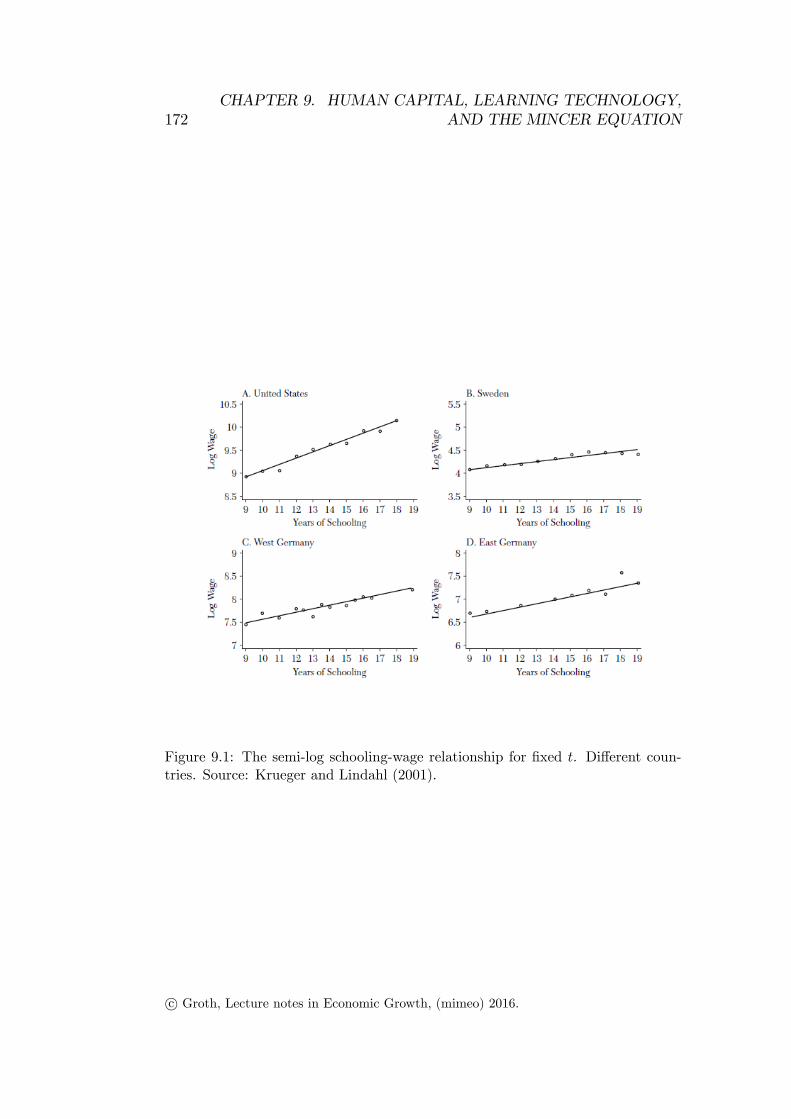
172CHAPTER 9. HUMAN CAPITAL, LEARNING TECHNOLOGY,
AND THE MINCER EQUATION
Figure 9.1: The semi-log schooling-wage relationship for fixed t. Different coun-tries. Source: Krueger and Lindahl (2001).
c© Groth, Lecture notes in Economic Growth, (mimeo) 2016.

9.4. What the Mincer equation is and is not 173
a wage profile, wt(S), such that a marginal condition analogue to (9.24) holdsfor all S for which there is a positive amount of labor traded in equilibrium,say all S ∈
[0, S
]:
dwt(S)/dS
wt(S)= r +m− g ≡ r for all S ∈
[0, S
]. (9.28)
It is here assumed, in the spirit of assumption A4 above, that technicalprogress implies that wt(S) for fixed S grows at the rate g, i.e., wt(S) =w0(S)egt, for all S ∈
[0, S
]. The equation (9.28) is a linear differential equa-
tion for wt w.r.t. S, defined in the interval 0 ≤ S ≤ S, while t is fixed. Andthe function wt(S) is the so far unknown solution to this differential equa-tion. That is, we have a differential equation of the form dx(S)/dS = rx(S),where the unknown function, x(S), is a function of schooling length ratherthan calendar time. The solution is x(S) = x(0)erS. Replacing the functionx(·) with the function wt(·), we thus have the solution
wt(S) = wt(0)erS. (9.29)
Note that in the previous section, in the context of (9.24), we requiredthe proportionate marginal return to schooling to equal r only for a specificS, i.e.,
d(wth(S))/dS
wth(S)=h′(S)
h(S)= r +m− g ≡ r for S = S∗. (9.30)
This is no more than a first-order condition assumed to hold at some point,S∗. It will generally not be a differential equation the solution of which gives aMincerian exponential relationship. A differential equation requires a deriv-ative relationship to hold not only at one point, but in an interval for theindependent variable (S in (9.28)). Indeed, in (9.28) we require the propor-tionate marginal return to schooling to equal r in a whole interval of schoolinglevels. Otherwise, with heterogeneity in the jobs offered, there could not beequilibrium.13
Returning to (9.29), by taking logs on both sides and substituting r byλ, we get (9.27), which is the Mincer equation in semi-loglinear form.As mentioned, empirically, the Mincer equation does surprisingly well in
cross-section regression analysis, cf. Figure 9.1.14 Note that (9.29) also yieldsa theory of how the “Mincerian slope”, λ, in (9.26) is determined, namely as
13It seems that Acemoglu (2009, p. 362) makes the logical error of identifying a first-order condition, (9.30), with a differential equation, (9.28).14The slopes are in the interval (0.05, 0.15).
c© Groth, Lecture notes in Economic Growth, (mimeo) 2016.

174CHAPTER 9. HUMAN CAPITAL, LEARNING TECHNOLOGY,
AND THE MINCER EQUATION
the mortality- and growth-corrected real interest rate, r. The evidence forthis part of the theory is more scarce.
Given the equilibrium educational wage profile, wt(S), the human wealthof an individual “born”at time 0 can be written
HW0 =
∫ ∞S
wt(0)erSe−(r+m)tdt = erS∫ ∞S
w0(0)egte−(r+m)tdt
= w0(0)erS∫ ∞S
e[g−(r+m)]tdt = w0(0)erS[e[g−(r+m)]t
g − (r +m)
]∞S
=w0(0)
r +m− g , (9.31)
since r ≡ r+m−g. In equilibrium the human wealth of the individual is thusindependent of S (within an interval) according to the Mincerian theory. Thisis due to “compensating wage differentials”, that is, the adjustment of theS-dependent wage levels so as to compensate for the S-dependent differencesin length of work life after schooling. Indeed, the essence of Mincer’s theoryis that if one level of schooling implies a higher human wealth than the otherlevels of schooling, the number of individuals choosing that level of schoolingwill rise until the associated wage has been brought down so as to be inline with the human wealth associated with the other levels of schooling. Ofcourse, such adjustment processes must in practice be quite time consumingand can only be approximative. Moreover, who among the ex ante similarindividuals ends up with what schooling level is indeterminate in this setup.
In this context, the original schooling technology, h(·), for human capitalformation has lost any importance. It does not enter human wealth in a long-run equilibrium in this disaggregate model where human wealth is simplygiven by (9.31). In this equilibrium people have different S’s and the receivedwage of an individual per unit of work has no relationship with the humancapital production function, h(·), by which we started in this section.Although there thus exists a microeconomic theory behind a Mincerian
relationship, this theory gives us a relationship for relative wages in a cross-section at a given point in time. It leaves open what an intertemporal pro-duction function for human capital, relating educational investment, S, to aresulting level, h, of labor effi ciency, looks like. Besides, the Mincerian slope,r, is a market price, not an aspect of schooling technology.
We have up to now been silent about the fact that our simple frameworkin Section 9.3 does not fully embrace the case of strong convexity implied byan exponential specification of h(S). Appendix B briefly comments.
c© Groth, Lecture notes in Economic Growth, (mimeo) 2016.
9.5. Empirics relating to h(S) 175
9.5 Empirics relating to h(S)
The empirical macroeconomic literature typically measures S as the averagenumber of years of schooling in the working-age population, taken for instancefrom the Barro and Lee (2001) data set.15
In their cross-country regression analysis de la Fuente and Domenech(2006) find a relationship essentially like that in Example 3 with η = 1. Theauthors find that the elasticity of GDP w.r.t. average years in school in thelabor force is at least 0.60.Similarly, the cross-country study, based on calibration, by Bills and
Klenow (2000) as well as the time series study by Cervelatti and Sunde(2010) favor the hypothesis of diminishing returns to schooling. Accordingto this, the linear term, rS, in the exponent in (9.26) should be replaced bya strictly concave function of S. These findings are in accordance with theresults by Psacharopoulus (1994). They give empirical reasons for scepticismtowards the linearity in h assumed in Example 2 of Section 9.2.For S > 0, the power function in Example 5 can be written h = Sη = eη lnS
and is thus in better harmony with the data than the exponential function(9.26). A parameter indicating the quality of schooling may be added: h =aeη lnS, where a > 0 may be a function of the teacher-pupil ratio, teachingmaterials per student etc. See Caselli (2005).
9.6 Concluding remarks
Our formulation of the schooling length decision problem in Section 9.3 con-tained several simplifications such that we ended up with a static maximiza-tion problem in Section 9.3.3. More general setups lead to truly dynamichuman capital accumulation problems.This chapter considered human capital as a productivity-enhancing fac-
tor. There is a partly complementary perspective on human capital, oftennamed the Nelson-Phelps hypothesis about the key role of human capitalfor technology adoption and technological catching up. An increase in hu-man capital leads to an increase in the technology absorption capability of anation.A simple way of formalizing this idea is obtained by recognizing that it
is not obvious that technical knowledge and human capital should enter theproduction function in the simple multiplicative way, Y = F (K,AhL), as
15This means that complicated aggregation issues, arising from cohort heterogeneityand from the fact that individual human capital is lost upon death, are bypassed. Fordiscussion, see Growiec and Groth (2015).
c© Groth, Lecture notes in Economic Growth, (mimeo) 2016.

176CHAPTER 9. HUMAN CAPITAL, LEARNING TECHNOLOGY,
AND THE MINCER EQUATION
assumed in (9.5) above. The complementarity between A and h may takeanother form, perhaps better reflecting that workers with high skill level canuse more advanced technology than workers with low skill level:
Y = F (K,hL, t) = F (K,min(h/η(A), 1)AL), η′(A) > 0,
where η(A) is the level of human capital required to fully exploit the currenttechnology level, A. If actual h < η(A), only the fraction h/η(A) of A isutilized. Similar ideas are sketched in Jones and Vollrath (2013, Ch. 6.1)and Acemoglu (2009, Ch. 10.8). See also Exercise V.3.Models based on the life-cycle approach to human capital typically con-
clude that education is productivity enhancing, i.e., more education has apositive level effect on income per capita but can only temporarily raise theper capita growth rate. Education is not a factor which in itself can explainsustained per capita growth. A more plausible main driving factor behindgrowth rather seems to be technological innovations. A higher level of percapita human capital may raise the speed of innovations, however. Thesethemes are taken up in the next chapter (and in Exercise V.7 and V.8).
9.7 Appendix
Appendix A
Suppose S = S∗ > 0 satisfies the first-order condition (9.24). To check thesecond-order condition, we consider
∂2HW
∂S2(v, S∗)
=∂HW
∂S(v, S∗)
[h′(S∗)
h(S∗)− (r +m− g)
]+HW (v, S∗)
h(S∗)h′′(S∗)− h′(S∗)2
h(S∗)2
= HW (v, S∗)
S∗
h′(S∗)h′′(S∗)− S∗
h(S∗)h′(S∗)
S∗h(S∗)h′(S∗), (9.32)
since the first term on the right-hand side in the second row vanishes due to(9.24) being satisfied at S = S∗. The second-order condition, ∂2HW/∂S2 < 0at S = S∗ holds if and only if the elasticity of h w.r.t. S exceeds that of h′
w.r.t. S at S = S∗. A suffi cient but not necessary condition for this is thath′′ ≤ 0. Anyway, since HW (v, S) is a continuous function of S, if there isa unique S∗ > 0 satisfying (9.24), and if ∂2HW/∂S2 < 0 holds for this S∗,then this S∗ is the unique optimal length of education for the individual.
c© Groth, Lecture notes in Economic Growth, (mimeo) 2016.
9.8. Literature 177
Appendix B
As alluded to at the end of Section 9.4, the strong convexity implied bythe exponential specification h(S) = h(0)eλS does not fit entirely well withthe model in Section 9.3 based on the “perpetual youth”assumption of age-independent mortality and no retirement. The problem is that when h(S)= h(0)eλS, the “perpetual youth”setup implies that the first-order condition(9.24) holds for all S; moreover, we get ∂2HW/∂S2 = 0 for all S.This problem reflects a limitation of the “perpetual youth”setup, where
there is no conclusive upper bound for anyone’s lifetime. It is not an argumentfor apriori rejection of the exponential specification.
9.8 Literature
Barro, R.J., and J. Lee, 2001, International data on educational attainment,Oxford Economic Papers, vol. 53 (3), 541-563.
Barro, R.J., and X. Sala-i-Martin, 2004, Economic Growth, 2nd edition,MIT Press.
Ben-Porath, Y., 1967, The production of human capital and the life cycleof earnings, Journal of Political Economy 75 (4), 352-365.
Bils, M., and P. J. Klenow, 2000. Does schooling cause growth? AmericanEconomic Review, 90 (5), 1160-1183.
Blanchard, O., 1985, J. Political Economy,
Browning, M., L.P. Hansen, and J.J. Heckman, 199, Micro data and generalequilibrium models. In: Handbook of macroecomics, vol. , ed. by...., 543-633.
Caselli, F., 2005, Accounting for cross-country income differences. In: Hand-book of Economic Growth, vol. IA.
Cervellati, M., and U. Sunde, 2010, Longevity and lifetime labor supply:Evidence and implications revisited, WP.
Cohen, D., and M. Soto, 2007, Growth and human capital: good data, goodresults, Journal of Economic Growth 12, 51-76.
Cunha, F., J.J. Heckman, L. Lochner, and D.V. Masterov, 2006, Interpret-ing the evidence on life cycle skill formation, Handbook of the Eco-nomics of Education, vol. 1, Amsterdam: Elsevier.
c© Groth, Lecture notes in Economic Growth, (mimeo) 2016.

178CHAPTER 9. HUMAN CAPITAL, LEARNING TECHNOLOGY,
AND THE MINCER EQUATION
Dalgaard, C.-J., and C.-T. Kreiner, 2001, Is declining productivity in-evitable? J. Econ. Growth, vol. 6 (3), 187-203.
de la Fuente, A., and R. Domenech, 2006, Human capital in growth re-gressions: How much difference does quality data make, Journal of theEuropean Economic Association 4 (1), 1-36.
Gemmell, N., 1996, , Oxford Bulletin of Economics and Statistics 58,9-28.
Growiec, J., 2010, Human capital, aggregation, and growth,MacroeconomicDynamics 14, 189-211.
Growiec, J., and C. Groth, 2015, On aggregating human capital acrossheterogeneous cohorts, Mathematical Social Sciences, vol. 78, 21-38.
Hall, R., and C.I. Jones, 1999, , Quarterly Journal of Economics.
Hanushek, E.A., and L. Woessmann, 2012, Do better schools lead to moregorwth? Cognitive skills, economic outcomes, and causation, J. Econ.Growth, vol. 17, 267-321.
Hazan, M., 2009, Longevity and lifetime labor supply: Evidence and impli-cations, Econometrica 77 (6), 1829-1863.
Heckman, J.J., L.J. Lochner, and P.E. Todd, 2003, Fifty years of Mincerearnings regressions, NBER WP 9732.
Heijdra, B.J., and W.E. Romp, 2009, Journal of EconomicDynamics and Control 33, 725-744.
Hendry, D., and H. Krolzig, 2004, We ran one regression, Oxford Bulletinof Economics and Statistics 66 (5), 799-810.
Jones, B., 2015, The human capital stock: A generalized approach, Ameri-can Economic Review.
Jones, C. I., 2005, Handbook of Economic Growth,
Jones, C. I., 2007, A simple Mincerian approach to endogenizing schooling,WP.
Krueger, A. B., and M. Lindahl, 2001. Education for growth: Why and forwhom? Journal of Economic Literature, 39, 1101-1136.
c© Groth, Lecture notes in Economic Growth, (mimeo) 2016.

9.8. Literature 179
Lucas, R.E., 1988, On the mechanics of economic development, Journal ofMonetary Economics 22, 3-42.
Lucas, R.E., 1993, Making a miracle, Econometrica 61, 251-272.
Mankiw, G., 1995,
Mankiw, G., D. Romer, and D. Weil, 1992, QJE.
Miles, D., 1999, Modelling the impact of demographic change upon theeconomy, Economic Journal 109, 1-36.
Mincer, J., 1958,
Mincer, J., 1974, Schooling, Experience, and Earnings, New York: NBERPress,
Ortigueira, S., 2003, Equipment prices, human capital and economic growth,Journal of Economic Dynamics and Control 28, 307-329.
Pritchett, L., 2006,
Psacharopoulus, 1994,
Rosen, S., 1976. A Theory of Life Earnings, JPE 84 (4), S45-S67.
Rosen, S., 2008. Human capital. In: The New Palgrave Dictionary ofEconomics, 2nd ed., ed. by S. N. Durlauf and L. E. Blume, availableat
http://www.econ.ku.dk/english/libraries/links/
Rosenzweig, M.R., 2010, Microeconomic approaches to development: School-ing, learning, and growth, Economic Growth Center Discussion PaperNo. 985, Yale University.
Sattinger, M., 1980, Capital and the Distribution of Labor Earnings, North-Holland: Amsterdam.
Sen, A., 1997,
Sheshinski, E., 2007, The Economic Theory of Annuities, Princeton: Prince-ton University Press.
Sheshinski, E., 2009, Uncertain longevity and investment in education, WP,The Hebrew University of Jerusalem, August.
c© Groth, Lecture notes in Economic Growth, (mimeo) 2016.

180CHAPTER 9. HUMAN CAPITAL, LEARNING TECHNOLOGY,
AND THE MINCER EQUATION
Sianesi, B., and J. Van Reenen, 2003, The returns to education: Macroeco-nomics, Journal of Economic Surveys 17 (2), 157-200.
–
c© Groth, Lecture notes in Economic Growth, (mimeo) 2016.

Chapter 11
AK and reduced-form AKmodels. Consumption taxation
The simplest model featuring “fully-endogenous”exponential per capita growthis what is known as the AK model. Jones and Vollrath (2013, Chapter 9, in-troduce a “Solow-style”AK model. Acemoglu (2009, Chapter 11) discussesAK and reduced-form AK models within a framework with Ramsey-stylehouseholds (i.e., a representative agent approach). The name “AK”refers toa special feature of the aggregate production function, namely the absenceof diminishing returns to capital. A characteristic result from AK models isthat they have no transitional dynamics.With the aim of synthesizing the formal characteristics of Ramsey-style
AK models, this lecture note gives a brief account of the common featuresof AK models and reduced-form AK models (Section 11.1 and 11.2, respec-tively). Finally, for later application we discuss in Section 11.3 conditionsunder which consumption taxation is not distortionary. Notation is standard.
11.1 General equilibrium dynamics in the sim-ple AK model
In the simple AK model we imagine a fully automatized economy where theaggregate production function is
Y (t) = AK(t), A > 0 and constant, (11.1)
so that marginal productivity of capital is
∂Y (t)
∂K(t)= A.
195

196CHAPTER 11. AK AND REDUCED-FORM AK
MODELS. CONSUMPTION TAXATION
There are thus constant returns to capital, not diminishing returns. Andlabor is no longer a production factor. The model should be considered athought experiment, not a model of reality.This section provides a detailed proof that when we embed the AK tech-
nology (11.1) in a Ramsey framework with perfect competition, the modelgenerates balanced growth from the beginning. So there will be no transi-tional dynamics.We consider a closed economy with perfect competition and no govern-
ment sector. The dynamic resource constraint for the economy is
K(t) = Y (t)−c(t)L(t)−δK(t) = AK(t)−c(t)L(t)−δK(t), K(0) > 0 given,(11.2)
where L(t) is population size. With the aim of maximizing profit, the repre-sentative firm demands capital services according to
Kd(t) =
∞ if r(t) + δ < A,
undetermined if r + δ = A,0 if r(t) + δ > A.
(11.3)
So, in equilibrium (Kd(t) = K(t)), the interest rate is r(t) = A − δ ≡r. With Ramsey households with rate of time preference, ρ, and constantelasticity of marginal utility of consumption, θ, we thus find the equilibriumgrowth rate of per capita consumption to be
c(t)
c(t)=
1
θ(r(t)− ρ) ≡ 1
θ(A− δ − ρ) ≡ gc, (11.4)
a constant. To ensure positive growth we impose the parameter restriction
A− δ > ρ. (A1)
And to ensure boundedness of discounted utility (and thereby a possibilityof satisfying the transversality condition of the representative household), weimpose the additional parameter restriction:
ρ− n > (1− θ)gc. (A2)
Reordering givesr = θgc + ρ > gc + n, (11.5)
where the equality is due to (16.27).Solving the linear differential equation (16.27) gives
c(t) = c(0)egct, (11.6)
c© Groth, Lecture notes in Economic Growth, (mimeo) 2016.

11.1. General equilibrium dynamics in the simple AK model 197
where c(0) is unknown so far (because c is not a predetermined variable).We shall find c(0) by appealing to the household’s transversality condition,
limt→∞
a(t)e−(r−n)t = 0, (TVC)
where a(t) is per capita financial wealth at time t. Recalling the No-Ponzi-Game condition,
limt→∞
a(t)e−(r−n)t ≥ 0, (NPG)
we see that the transversality condition is equivalent to the No-Ponzi-Gamecondition being not over-satisfied.Defining k(t) ≡ K(t)/L(t), the dynamic resource constraint, (11.2), is in
per-capita terms
k(t) = (A− δ − n)k(t)− c(0)egct, k(0) > 0 given, (11.7)
where we have inserted (12.24). The solution to this linear differential equa-tion is (cf. Appendix to Chapter 3)
k(t) =
(k(0)− c(0)
r − n− gc
)e(r−n)t +
c(0)
r − n− gcegct, r ≡ A− δ. (11.8)
In our closed-economy framework with no public debt, a(t) = k(t). So thequestion is: When will the time path (11.8) satisfy (TVC) with a(t) = k(t)?To find out, we multiply by the discount factor e−(r−n)t on both sides of (11.8)to get
k(t)e−(r−n)t = k(0)− c(0)
r − n− gc+
c(0)
r − n− gce−(r−gc−n)t.
Thus, in view of the assumption (A2), (11.5) holds and thereby the last termon the right-hand side vanishes for t→∞. Hence
limt→∞
k(t)e−(r−n)t = k(0)− c(0)
r − n− gc.
From this we see that the representative household satisfies (TVC) if andonly if it chooses
c(0) = (r − n− gc)k(0). (11.9)
This is the equilibrium solution for the household’s chosen per capita con-sumption at time t = 0. If the household instead had chosen c(0) < (r−n−gc)k(0), then limt→∞ k(t)e−(r−n)t > 0 and so the household would not satisfy(TVC) but instead be over-saving. And if it had chosen c(0)> (r−n−gc)k(0),
c© Groth, Lecture notes in Economic Growth, (mimeo) 2016.

198CHAPTER 11. AK AND REDUCED-FORM AK
MODELS. CONSUMPTION TAXATION
then limt→∞ k(t)e−(r−n)t < 0 and so the household would be over-consumingand violate (NPG) (hence also (TVC)).Substituting the solution for c(0) into (11.8) gives the evolution of k(t)
in equilibrium,
k(t) =c(0)
r − n− gcegct = k(0)egct.
So from the beginning k grows at the same constant rate as c. Since percapita output is y ≡ Y/L = Ak, the same is true for per capita output.Hence, from start the system is in balanced growth (there is no transitionaldynamics).The AK model features one of the simplest kinds of endogenous growth
one can think of. Exponential growth is endogenous in the model in thesense that there is positive per capita growth in the long run, generated byan internal mechanism in the model (not by exogenous technology growth).The endogenously determined capital accumulation constitutes the mecha-nism through which sustained per capita growth is generated and sustained.It is because the net marginal productivity of capital is assumed constantand, according to (A1), higher than the rate of impatience, ρ, that capitalaccumulation itself is so powerful.
11.2 Reduced-form AK models
The models known as reduced-form AK models are a generalization of thesimple AK model considered above. In contrast to the simple AK model,where only physical capital is an input, a reduced-form AK model assumesa technology involving at least two different inputs. Yet it is possible thatin general equilibrium the aggregate production function ends up implyingproportionality between output and some measure of “broad capital”, i.e.,
Y (t) = BK(t),
where B is some endogenously determined positive constant, and K(t) is“broad capital”. If in addition the real interest rate in general equilibriumends up being a constant, the model is called a reduced-form AK model. In thesimple AK model constancy of average productivity of capital is postulatedfrom the beginning. In the reduced-form AKmodels the average productivityof capital becomes and remains endogenously constant over time.An example is the “AK model with physical and human capital”in Ace-
moglu, Chapter 11.2. With Ramsey-style households and the formation ofhuman capital treated as similar to that of physical capital, Acemoglu finds
c© Groth, Lecture notes in Economic Growth, (mimeo) 2016.
11.2. Reduced-form AK models 199
that along the balanced growth path (obtained after an initial phase with fullspecialization in either physical or human capital accumulation), we have1
Y (t) = F (K(t), h(t)L(t)) = f(k∗)h(t)L(t) = f(k∗)H(t), (11.10)
where we have defined
k ≡ K
H≡ K
hL≡ k
h.
We further define
K(t) ≡ K(t) +H(t) = “broad capital”.
Then
K(t) ≡ (K(t)
H(t)+ 1)H(t) = (k∗ + 1)H(t),
along the BGP. Isolating H(t) and inserting into (11.10) gives
Y (t) = f(k∗)1
k∗ + 1K(t) ≡ BK(t).
At an abstract level it is thus conceivable that “broad capital”, defined asthe sum of physical and human capital, can be meaningful. Empirically,however, there exists no basis for believing this concept of “broad capital”to be useful, cf. Exercises V.4 and V.5.Anyway, a reduced-form AK model ends up with quite similar aggregate
relations as those in the simple AK model. Hence the solution procedure tofind the equilibrium path is quite similar to that in the simple AK modelabove. Again there will be no transitional dynamics.2
The nice feature of AKmodels is that they provide very simple theoreticalexamples of endogenous growth. The problematic feature is that they tendto simplify the technology description too much. They constitute extremeknife-edge cases, not something intermediate. This weakness also character-izes so-called asymptotic AK models or asymptotic reduced-form AK models(Exercise I.7 provides simple examples).
1The mentioned initial phase is left unnoticed in Acemoglu. In our notation k ≡ K/L
and k ≡ K/H, while Acemoglu’s text has k ≡ K/H.2See Chapter 12.3. See also Exercise VI.4.
c© Groth, Lecture notes in Economic Growth, (mimeo) 2016.

200CHAPTER 11. AK AND REDUCED-FORM AK
MODELS. CONSUMPTION TAXATION
11.3 On consumption taxation
As a preparation for the discussion shortly in this course of fiscal policy inrelation to economic growth, we shall here try to clarify an aspect of con-sumption taxation. This is the question: is a consumption tax distortionary- always? never? sometimes?The answer is the following.1. Suppose labor supply is elastic (due to leisure entering the utility
function). Then a consumption tax (whether constant or time-dependent)is generally distortionary, creating a wedge between the MRS between con-sumption and leisure and labor’s marginal productivity. The tax reduces theeffective opportunity cost of leisure by reducing the amount of consumptionforgone by working one hour less. Indeed, the tax makes consumption goodsmore expensive and so the amount of consumption that the agent can buyfor the hourly wage becomes smaller. The substitution effect on leisure of aconsumption tax is thus positive, while the income and wealth effects will benegative. Generally, the net effect will not be zero, but it can be of any sign;it may be small in absolute terms.2. Suppose labor supply is inelastic (no trade-off between consumption
and leisure). Then, at least in the type of growth models we consider in thiscourse, a constant (time-independent) consumption tax acts as a lump-sumtax and is thus non-distortionary. If the consumption tax is time-dependent,however, a distortion of the intertemporal aspect of household decisions tendsto arise.To understand answer 2, consider a Ramsey household with inelastic labor
supply. Suppose the household faces a time-varying consumption tax rateτ t > 0. To obtain a consumption level per time unit equal to ct per capita,the household has to spend
ct = (1 + τ t)ct
units of account (in real terms) per capita. Thus, spending ct per capita pertime unit results in the per capita consumption level
ct = (1 + τ t)−1ct. (11.11)
In order to concentrate on the consumption tax as such, we assume thetax revenue is simply given back as lump-sum transfers and that there areno other government activities. Then, with a balanced government budget,we have
xtLt = τ tctLt,
c© Groth, Lecture notes in Economic Growth, (mimeo) 2016.

11.3. On consumption taxation 201
where xt is the per capita lump-sum transfer, exogenous to the household,and Lt is the size of the representative household.Assuming CRRA utility with parameter θ > 0, the instantaneous per
capita utility can be written
u(ct) =c1−θt − 1
1− θ =(1 + τ t)
θ−1c1−θt − 1
1− θ .
In our standard notation the household’s intertemporal optimization prob-lem, in continuous time, is then to choose (ct)
∞t=0 so as to maximize
U0 =
∫ ∞0
(1 + τ t)θ−1c1−θ
t − 1
1− θ e−(ρ−n)tdt s.t.
ct ≥ 0,
at = (rt − n)at + wt + xt − ct, a0 given,
limt→∞
ate−∫∞0 (rs−n)ds ≥ 0.
From now, we let the timing of the variables be implicit unless needed forclarity. The current-value Hamiltonian is
H =(1 + τ)θ−1c1−θ − 1
1− θ + λ [(r − n)a+ w + x− c] ,
where λ is the co-state variable associated with financial per capita wealth,a. An interior optimal solution will satisfy the first-order conditions
∂H
∂c= (1 + τ)θ−1c−θ − λ = 0, so that (1 + τ)θ−1c−θ = λ, (11.12)
∂H
∂a= λ(r − n) = −λ+ (ρ− n)λ, (11.13)
and a transversality condition which amounts to
limt→∞
ate−∫∞0 (rs−n)ds = 0. (11.14)
We take logs in (11.12) to get
(θ − 1) log(1 + τ)− θ log c = log λ.
Differentiating w.r.t. time, taking into account that τ = τ t, gives
(θ − 1)τ
1 + τ− θ
·c
c=λ
λ= ρ− r.
c© Groth, Lecture notes in Economic Growth, (mimeo) 2016.

202CHAPTER 11. AK AND REDUCED-FORM AK
MODELS. CONSUMPTION TAXATION
By ordering, we find the growth rate of consumption spending,·c
c=
1
θ
[r + (θ − 1)
τ
1 + τ− ρ].
Using (11.11), this gives the growth rate of consumption,
c
c=
·c
c− τ
1 + τ=
1
θ
[r + (θ − 1)
τ
1 + τ− ρ]− τ
1 + τ=
1
θ(r − τ
1 + τ− ρ).
Assuming firms maximize profit under perfect competition, in equilibriumthe real interest rate will satisfy
r =∂Y
∂K− δ. (11.15)
But the effective real interest rate, r, faced by the consuming household, is
r = r − τ
1 + τQ r for τ R 0,
respectively. If for example the consumption tax is increasing, then the effec-tive real interest rate faced by the consumer is smaller than the market realinterest rate, given in (11.15), because saving implies postponing consump-tion and future consumption is more expensive due to the higher consumptiontax rate.The conclusion is that a time-varying consumption tax rate is distor-
tionary. It implies a wedge between the intertemporal rate of transformationfaced by the consumer, reflected by r, and the intertemporal rate of transfor-mation available in the technology of society, indicated by r in (11.15). Onthe other hand, if the consumption tax rate is constant, the consumptiontax is non-distortionary when there is no utility from leisure.
A remark on tax smoothingIn models with transitional dynamics it is often so that maintaining constanttax rates is inconsistent with maintaining a balanced government budget. Isthe implication of this that we should recommend the government to let taxrates be continually adjusted so as to maintain a forever balanced budget?No! As the above example as well as business cycle theory suggest, maintain-ing tax rates constant (“tax smoothing”), and thereby allowing governmentdeficits and surpluses to arise, will generally make more sense. In itself, abudget deficit is not worrisome. It only becomes worrisome if it is not accom-panied later by suffi cient budget surpluses to avoid an exploding governmentdebt/GDP ratio to arise. This requires that the tax rates taken togetherhave a level which in the long run matches the level of government expenses.
c© Groth, Lecture notes in Economic Growth, (mimeo) 2016.

Chapter 12
Learning by investing: two
versions
The learning-by-investing model, sometimes called the learning-by-doing model,
is one of the basic endogenous growth models. By basic is meant that the
model specifies not only the technological aspects of the economy but also
the market structure and the household sector, including household prefer-
ences. As in much other endogenous growth theory, the modeling of the
household sector follows Ramsey and assumes the existence of a representa-
tive infinitely-lived household. Since this results in a simple determination
of the long-run interest rate (the modified golden rule), the analyst can in a
first approach concentrate on the main issue, technological change, without
being detracted by aspects secondary to this issue.
In the present model learning from investment experience and diffusion
across firms of the resulting new technical knowledge (positive externalities)
play a key role.
There are two popular alternative versions of the model. The distinguish-
ing feature is whether the learning parameter (see below) is less than one or
equal to one. The first case corresponds to (a simplified version of) a model
by Nobel laureate Kenneth Arrow (1962). The second case has been drawn
attention to by Paul Romer (1986) who assumes that the learning parameter
equals one. These two contributions start out from a common framework
which we now present.1
1This lecture note also contains, in the appendix, a refresher on the concepts of a saddle
point and saddle point stability.
203
204
CHAPTER 12. LEARNING BY INVESTING:
TWO VERSIONS
12.1 The common framework
We consider a closed economy with firms and households interacting under
conditions of perfect competition. Later, a government attempting to inter-
nalize the positive investment externality is introduced.
Let there be firms in the economy ( “large”). Suppose they all have
the same neoclassical production function, with CRS. Firm no. faces the
technology
= ( ) = 1 2 (12.1)
where the economy-wide technology level is an increasing function of so-
ciety’s previous experience, proxied by cumulative aggregate net investment:
=
µZ
−∞
¶
= 0 ≤ 1 (12.2)
where is aggregate net investment and =P
2
The idea is that investment − the production of capital goods − as anunintended by-product results in experience or what we may call on-the-job
learning. Experience allows producers to recognize opportunities for process
and quality improvements. In this way knowledge is achieved about how to
use the new capital goods efficiently and how to produce them in a cost-
efficient way. This includes learning how to improve their design so that in
combination with labor they are more productive and better satisfy the needs
of the users. As formulated by Arrow:
“each newmachine produced and put into use is capable of chang-
ing the environment in which production takes place, so that
learning is taking place with continually new stimuli” (Arrow,
1962).3
The learning is assumed to benefit producers in many lines of produc-
tion in the economy: learning by doing, learning by watching, learning by
using. There are knowledge spillovers across firms and these spillovers are
2With arbitrary units of measurement for labor and output, the hypothesis is =
0 In (12.2) measurement units are chosen such that = 1.3Concerning empirical evidence of learning-by-doing and learning-by-investing, see
Chapter 13. The citation of Arrow indicates that it was rather experience from cumu-
lative gross investment he had in mind as the basis for learning. Yet the hypothesis in
(12.2) is the more popular one - seemingly for no better reason than that it leads to
simpler dynamics. Another way in which (12.2) deviates from Arrow’s original ideas is
by assuming that technical progress is disembodied rather than embodied, an important
distinction we defined in Chapter 2.2.
c° Groth, Lecture notes in Economic Growth, (mimeo) 2016.

12.1. The common framework 205
reasonably fast relative to the time horizon relevant for growth theory. In
our macroeconomic approach both and are in fact assumed to be exactly
the same for all firms in the economy. That is, in this specification the firms
producing consumption-goods benefit from the learning just as much as the
firms producing capital-goods.
The parameter indicates the elasticity of the general technology level,
with respect to cumulative aggregate net investment and is named the
“learning parameter”. Whereas Arrow assumes 1 Romer focuses on the
case = 1 The case of 1 is ruled out since it would lead to explosive
growth (infinite output in finite time) and is therefore not plausible.
12.1.1 The individual firm
In the simple Ramsey model we assumed that households directly own the
capital goods in the economy and rent them out to the firms. When dis-
cussing learning-by-investment, it somehow fits the intuition better if we
(realistically) assume that the firms generally own the capital goods they
use. They then finance their capital investment by issuing shares and bonds.
Households’ financial wealth then consists of these shares and bonds.
Consider firm There is perfect competition in all markets. So the firm
is a price taker. Its problem is to choose a production and investment plan
which maximizes the present value, of expected future cash-flows. Thus
the firm chooses ( )∞=0 to maximize
0 =
Z ∞
0
[ ( )− − ] −
0
subject to = − Here and are the real wage and gross
investment, respectively, at time , is the real interest rate at time and
≥ 0 is the capital depreciation rate. Rising marginal capital installationcosts and other kinds of adjustment costs are assumed minor and can be
ignored. It can be shown that in this case the firm’s problem is equivalent
to maximization of current pure profits in every short time interval. So, as
hitherto, we can describe the firm as just solving a series of static profit
maximization problems.
We suppress the time index when not needed for clarity. At any date firm
maximizes current pure profits, Π = ( )− ( + ) − This
leads to the first-order conditions for an interior solution:
Π = 1( )− ( + ) = 0 (12.3)
Π = 2( )− = 0
c° Groth, Lecture notes in Economic Growth, (mimeo) 2016.

206
CHAPTER 12. LEARNING BY INVESTING:
TWO VERSIONS
Behind (12.3) is the presumption that each firm is small relative to the econ-
omy as a whole, so that each firm’s investment has a negligible effect on
the economy-wide technology level . Since is homogeneous of degree
one, by Euler’s theorem,4 the first-order partial derivatives, 1 and 2 are
homogeneous of degree 0. Thus, we can write (12.3) as
1( ) = + (12.4)
where ≡ . Since is neoclassical, 11 0 Therefore (12.4) deter-
mines uniquely. From (12.4) follows that the chosen capital-labor ratio,
will be the same for all firms, say
12.1.2 The household
The representative household (or family dynasty) has = 0 members
each of which supplies one unit of labor inelastically per time unit, ≥ 0.The household has CRRA instantaneous utility with parameter 0 The
pure rate of time preference is a constant, . The flow budget identity in per
head terms is
= ( − ) + − 0 given,
where is per head financial wealth. The NPG condition is
lim→∞
−
0(−) ≥ 0
The resulting consumption-saving plan implies that per head consumption
follows the Keynes-Ramsey rule,
=1
( − )
and the transversality condition that the NPG condition is satisfied with
strict equality. In general equilibrium of our closed economy without natural
resources and government debt, will equal
4Recall that a function ( ) defined in a domain is homogeneous of degree if for
all ( ) in ( ) = ( ) for all 0 If a differentiable function ( ) is
homogeneous of degree then (i) 01( ) + 02( ) = ( ) and (ii) the first-order
partial derivatives, 01( ) and 02( ) are homogeneous of degree − 1.
c° Groth, Lecture notes in Economic Growth, (mimeo) 2016.
12.2. The arrow case: 1 207
12.1.3 Equilibrium in factor markets
In equilibriumP
= andP
= where and are the avail-
able amounts of capital and labor, respectively (both pre-determined). SinceP =
P =
P = the chosen capital-labor ratio, satisfies
= =
≡ = 1 2 (12.5)
As a consequence we can use (12.4) to determine the equilibrium interest
rate:
= 1( )− (12.6)
That is, whereas in the firm’s first-order condition (12.4) causality goes from
to in (12.6) causality goes from to Note also that in our closed
economy with no natural resources and no government debt, will equal
The implied aggregate production function is
=X
≡X
=X
( ) =X
() (by (12.1) and (12.5))
= ()X
= () = () = () (by (12.2)), (12.7)
where we have several times used that is homogeneous of degree one.
12.2 The arrow case: 1
The Arrow case is the robust case where the learning parameter satisfies
0 1 The method for analyzing the Arrow case is analogue to that
used in the study of the Ramsey model with exogenous technical progress.
In particular, aggregate capital per unit of effective labor, ≡ () is a
key variable. Let ≡ () Then
= ()
= ( 1) ≡ () 0 0 00 0 (12.8)
We can now write (12.6) as
= 0()− (12.9)
where is pre-determined.
c° Groth, Lecture notes in Economic Growth, (mimeo) 2016.

208
CHAPTER 12. LEARNING BY INVESTING:
TWO VERSIONS
12.2.1 Dynamics
From the definition ≡ () follows
·
=
−
−
=
−
− (by (12.2))
= (1− ) − −
− = (1− )
− −
− where ≡
≡
Multiplying through by we have
· = (1− )(()− )− [(1− ) + ] (12.10)
In view of (12.9), the Keynes-Ramsey rule implies
≡
=1
( − ) =
1
³ 0()− −
´ (12.11)
Defining ≡ now follows
=
−
=
−
=
−
− −
=
−
( − − )
=1
( 0()− − )−
( − − )
Multiplying through by we have
· =
∙1
( 0()− − )−
(()− − )
¸ (12.12)
The two coupled differential equations, (12.10) and (12.12), determine
the evolution over time of the economy.
Phase diagram
Figure 12.1 depicts the phase diagram. The· = 0 locus comes from (12.10),
which gives· = 0 for = ()− ( +
1− ) (12.13)
where we realistically may assume that + (1 − ) 0 As to the· = 0
locus, we have
· = 0 for = ()− −
( 0()− − )
= ()− −
≡ () (from (12.11)). (12.14)
c° Groth, Lecture notes in Economic Growth, (mimeo) 2016.

12.2. The arrow case: 1 209
*k GRk kk
c 0c
0k
B
E *c
0 k
Figure 12.1: Phase diagram for the Arrow model.
Before determining the slope of the· = 0 locus, it is convenient to consider
the steady state, (∗ ∗).
Steady state
In a steady state and are constant so that the growth rate of as well
as equals + i.e.,
=
=
+ =
+
Solving gives
=
=
1−
Thence, in a steady state
=
− =
1− − =
1− ≡ ∗ and (12.15)
=
=
1− = ∗ (12.16)
The steady-state values of and respectively, will therefore satisfy, by
(12.11),
∗ = 0(∗)− = + ∗ = +
1− (12.17)
c° Groth, Lecture notes in Economic Growth, (mimeo) 2016.

210
CHAPTER 12. LEARNING BY INVESTING:
TWO VERSIONS
To ensure existence of a steady state we assume that the private marginal
product of capital is sufficiently sensitive to capital per unit of effective labor,
from now called the “capital intensity”:
lim→0
0() + +
1− lim
→∞ 0() (A1)
The transversality condition of the representative household is that lim→∞
− 0(−) = 0 where is per capita financial wealth. In general equi-
librium = ≡ where in steady state grows according to (12.16).
Thus, in steady state the transversality condition can be written
lim→∞
∗(∗−∗+) = 0 (TVC)
For this to hold, we need
∗ ∗ + =
1− (12.18)
by (12.15). In view of (12.17), this is equivalent to
− (1− )
1− (A2)
which we assume satisfied.
As to the slope of the· = 0 locus we have, from (12.14),
0() = 0()− − 1( 00()
+ ) 0()− − 1 (12.19)
since 00 0 At least in a small neighborhood of the steady state we can
sign the right-hand side of this expression. Indeed,
0(∗)−−1∗ = +∗−
1
∗ = +
1− −
1− = −−(1−)
1− 0
(12.20)
by (12.15) and (A2). So, combining with (12.19), we conclude that 0(∗) 0By continuity, in a small neighborhood of the steady state, 0() ≈ 0(∗) 0
Therefore, close to the steady state, the· = 0 locus is positively sloped, as
indicated in Figure 12.1.
Still, we have to check the following question: In a neighborhood of the
steady state, which is steeper, the· = 0 locus or the
· = 0 locus? The slope
of the latter is 0()− − (1− ) from (12.13) At the steady state this
slope is
0(∗)− − 1∗ ∈ (0 0(∗))
c° Groth, Lecture notes in Economic Growth, (mimeo) 2016.

12.2. The arrow case: 1 211
in view of (12.20) and (12.19). The· = 0 locus is thus steeper. So, the
· = 0
locus crosses the· = 0 locus from below and can only cross once.
The assumption (A1) ensures existence of a ∗ 0 satisfying (12.17). AsFigure 12.1 is drawn, a little more is implicitly assumed namely that there
exists a 0 such that the private net marginal product of capital equals
the steady-state growth rate of output, i.e.,
0()− = (
)∗ = (
)∗ +
=
1− + =
1− (12.21)
where we have used (12.16). Thus, the tangent to the· = 0 locus at =
is horizontal and ∗ as indicated in the figure.Note, however, that is not the golden-rule capital intensity. The latter
is the capital intensity, at which the social net marginal product of
capital equals the steady-state growth rate of output (see Appendix). If exists, it will be larger than as indicated in Figure 12.1. To see this, we
now derive a convenient expression for the social marginal product of capital.
From (12.7) we have
= 1(·) + 2(·)−1 = 0() + 2(·)(−1) (by (12.8))
= 0() + ( (·)− 1(·))−1 (by Euler’s theorem)
= 0() + (()− 0())−1 (by (12.8) and (12.2))
= 0() + (()−1− 0()) = 0() + ()− 0()
0()
in view of = () = 1−−1 and ()− 0() 0As expected, thepositive externality makes the social marginal product of capital larger than
the private one. Since we can also write = (1− ) 0() + ()
we see that is (still) a decreasing function of since both 0() and() are decreasing in So the golden rule capital intensity, will be
that capital intensity which satisfies
0() + ()−
0()
− =
Ã
!∗=
1−
To ensure there exists such a we strengthen the right-hand side inequal-
ity in (A1) by the assumption
lim→∞
à 0() +
()− 0()
! +
1− (A3)
c° Groth, Lecture notes in Economic Growth, (mimeo) 2016.

212
CHAPTER 12. LEARNING BY INVESTING:
TWO VERSIONS
This, together with (A1) and 00 0, implies existence of a unique , and
in view of our additional assumption (A2), we have 0 ∗ as
displayed in Figure 12.1.
Stability
The arrows in Figure 12.1 indicate the direction of movement, as determined
by (12.10) and (12.12)). We see that the steady state is a saddle point.
Moreover, the dynamic system is saddle-point stable.5 The dynamic system
has one pre-determined variable, and one jump variable, The saddle
path is not parallel to the jump variable axis. We claim that for a given
0 0 (i) the initial value of 0 will be the ordinate to the point where
the vertical line = 0 crosses the saddle path; (ii) over time the economy
will move along the saddle path towards the steady state. Indeed, this time
path is consistent with all conditions of general equilibrium, including the
transversality condition (TVC). And the path is the only technically feasible
path with this property. Indeed, all the divergent paths in Figure 12.1 can
be ruled out as equilibrium paths because they can be shown to violate the
transversality condition of the household.
In the long run and ≡ ≡ = (∗) grow at the rate (1−)which is positive if and only if 0 This is an example of endogenous growth
in the sense that the positive long-run per capita growth rate is generated
through an internal mechanism (learning) in the model (in contrast to exoge-
nous technology growth as in the Ramsey model with exogenous technical
progress).
12.2.2 Two types of endogenous growth
As also touched upon elsewhere in these lecture notes, it is useful to distin-
guish between two types of endogenous exponential growth. Fully endoge-
nous exponential growth occurs when the long-run growth rate of is positive
without support from growth in any exogenous factor; the Romer case, to
be considered in the next section, provides an example. Semi-endogenous
exponential growth occurs if growth is endogenous but a positive per capita
growth rate can not be maintained in the long run without the support
from growth in some exogenous factor (for example exogenous growth in the
labor force). Clearly, in the Arrow version of learning by investing, exponen-
tial growth is “only” semi-endogenous. The technical reason for this is the
assumption that the learning parameter, is below 1 which implies dimin-
ishing marginal returns to capital at the aggregate level. As a consequence,
5A formal definition is given in Appendix B.
c° Groth, Lecture notes in Economic Growth, (mimeo) 2016.
12.3. Romer’s limiting case: = 1 = 0 213
if and only if 0 do we have 0 in the long run. In line with this,
∗ 06
The key role of population growth derives from the fact that although
there are diminishing marginal returns to capital at the aggregate level, there
are increasing returns to scale w.r.t. capital and labor. For the increasing
returns to be exploited, growth in the labor force is needed. To put it dif-
ferently: when there are increasing returns to and together, growth in
the labor force not only counterbalances the falling marginal productivity of
aggregate capital (this counter-balancing role reflects the direct complemen-
tarity between and ), but also upholds sustained productivity growth via
the learning mechanism.
Note that in the semi-endogenous growth case, ∗ = (1− )2 0
for 0 That is, a higher value of the learning parameter implies higher
per capita growth in the long run, when 0. Note also that ∗ = 0= ∗ that is, in the semi-endogenous growth case, preference parametersdo not matter for the long-run per capita growth rate. As indicated by
(12.15), the long-run growth rate is tied down by the learning parameter,
and the rate of population growth, Like in the simple Ramsey model,
however, it can be shown that preference parameters matter for the level of
the growth path. For instance (12.17) shows that ∗ 0 so that more
patience (lower ) imply a higher ∗ and thereby a higher = (∗)
This suggests that although taxes and subsidies do not have long-run
growth effects, they can have level effects.
In this model there is clearly a motivation for government intervention
due to the positive externality of private investment. But details about the
design of government policy vis-a-vis this externality will in this lecture note
only be discussed in relation to the Romer case of = 1, which is simpler
and to which we now return.
12.3 Romer’s limiting case: = 1 = 0
We now consider the limiting case = 1We should think of it as a thought
experiment because, by most observers, the value 1 is considered an unrealis-
tically high value for the learning parameter. Moreover, in combination with
0 the value 1 will lead to a forever rising per capita growth rate which
does not accord the economic history of the industrialized world over more
6Note, however, that the model, and therefore (12.15), presupposes ≥ 0 If 0 the
steady-state formulas in Section 12.2 are no longer valid. The formula in (12.16) would
for instance imply a decreasing level of technical knowledge, which, at least in a modern
economy, is implausible.
c° Groth, Lecture notes in Economic Growth, (mimeo) 2016.

214
CHAPTER 12. LEARNING BY INVESTING:
TWO VERSIONS
than a century. To avoid a forever rising growth rate, we therefore introduce
the parameter restriction = 0
The resulting model turns out to be extremely simple and at the same
time it gives striking results (both circumstances have probably contributed
to its popularity).
First, with = 1 we get = and so the equilibrium interest rate is,
by (12.6),
= 1()− = 1(1 )− ≡
where we have divided the two arguments of 1() by ≡ and
again used Euler’s theorem. Note that the interest rate is constant “from the
beginning” and independent of the historically given initial value of 0.
The aggregate production function is now
= () = (1 ) constant, (12.22)
and is thus linear in the aggregate capital stock.7 In this way the general neo-
classical presumption of diminishing returns to capital has been suspended
and replaced by exactly constant returns to capital. Thereby the Romer
model belongs to the class of reduced-form AK models, that is, models where
in general equilibrium the interest rate and the aggregate output-capital ratio
are necessarily constant over time whatever the initial conditions.
The method for analyzing an AK model is different from the one used for
a diminishing returns model as above.
12.3.1 Dynamics
The Keynes-Ramsey rule now takes the form
=1
( − ) =
1
(1(1 )− − ) ≡ (12.23)
which is also constant “from the beginning”. To ensure positive growth, we
assume
1(1 )− (A1’)
And to ensure bounded intertemporal utility (and thereby a possibility of
satisfying the transversality condition of the representative household), it is
assumed that
(1− ) and therefore + = (A2’)
7Acemoglu, p. 400, writes this as = ()
c° Groth, Lecture notes in Economic Growth, (mimeo) 2016.

12.3. Romer’s limiting case: = 1 = 0 215
(1, )F L
K
Y
1
( , )F K L1(1, )F L
(1, )F L
Figure 12.2: Illustration of the fact that for given, (1 ) 1(1 )
Solving the linear differential equation (12.23) gives
= 0 (12.24)
where 0 is unknown so far (because is not a predetermined variable). We
shall find 0 by applying the households’ transversality condition
lim→∞
− = lim
→∞
− = 0 (TVC)
First, note that the dynamic resource constraint for the economy is
= − − = (1 ) − −
or, in per-capita terms,
= [ (1 )− ] − 0 (12.25)
In this equation it is important that (1 ) − − 0 To understand
this inequality, note that, by (A2’), (1 ) − − (1 ) − − =
(1 ) − 1(1 ) = 2(1 ) 0 where the first equality is due to
= 1(1 )− and the second is due to the fact that since is homogeneous
of degree 1, we have, by Euler’s theorem, (1 ) = 1(1 ) · 1 + 2(1 )
1(1 ) in view of (A1’). The key property (1 )− 1(1 ) 0 is
illustrated in Figure 12.2.
c° Groth, Lecture notes in Economic Growth, (mimeo) 2016.
216
CHAPTER 12. LEARNING BY INVESTING:
TWO VERSIONS
The solution of a general linear differential equation of the form () +
() = with 6= − is
() = ((0)−
+ )− +
+ (12.26)
Thus the solution to (12.25) is
= (0 − 0
(1 )− − )( (1)−) +
0
(1 )− − (12.27)
To check whether (TVC) is satisfied we consider
− = (0 − 0
(1 )− − )( (1)−−) +
0
(1 )− − (−)
→ (0 − 0
(1 )− − )( (1)−−) for →∞
since by (A2’). But = 1(1 )− (1 )− and so (TVC) is
only satisfied if
0 = ( (1 )− − )0 (12.28)
If 0 is less than this, there will be over-saving and (TVC) is violated (− →
∞ for → ∞ since = ). If 0 is higher than this, both the NPG and
(TVC) are violated (− → −∞ for →∞).
Inserting the solution for 0 into (12.27), we get
=0
(1 )− − = 0
that is, grows at the same constant rate as “from the beginning” Since
≡ = (1 ) the same is true for Hence, from start the system is
in balanced growth (there is no transitional dynamics).
This is a case of fully endogenous growth in the sense that the long-run
growth rate of is positive without the support by growth in any exogenous
factor. This outcome is due to the absence of diminishing returns to aggregate
capital, which is implied by the assumed high value of the learning parameter.
But the empirical foundation for this high value is weak, to say the least, cf.
Chapter 13. A further drawback of this special version of the learning model
is that the results are non-robust. With slightly less than 1, we are back
in the Arrow case and growth peters out, since = 0With slightly above
1, it can be shown that growth becomes explosive: infinite output in finite
time!8
8See Appendix B in Chapter 13.
c° Groth, Lecture notes in Economic Growth, (mimeo) 2016.

12.3. Romer’s limiting case: = 1 = 0 217
The Romer case, = 1 is thus a knife-edge case in a double sense. First,
it imposes a particular value for a parameter which apriori can take any value
within an interval. Second, the imposed value leads to non-robust results;
values in a hair’s breadth distance result in qualitatively different behavior
of the dynamic system.
Note that the causal structure in the long run in the diminishing returns
case is different than in the AK-case of Romer. In the diminishing returns
case the steady-state growth rate is determined first, as ∗ in (12.15), then∗ is determined through the Keynes-Ramsey rule and, finally, is de-
termined by the technology, given ∗ In contrast, the Romer case has and directly given as (1 ) and respectively. In turn, determines the
(constant) equilibrium growth rate through the Keynes-Ramsey rule
12.3.2 Economic policy in the Romer case
In the AK case, that is, the fully endogenous growth case, we have
0 and 0 Thus, preference parameters matter for the long-run
growth rate and not “only” for the level of the upward-sloping time path
of per capita output. This suggests that taxes and subsidies can have long-
run growth effects. In any case, in this model there is a motivation for
government intervention due to the positive externality of private investment.
This motivation is present whether 1 or = 1 Here we concentrate on
the latter case, for no better reason than that it is simpler. We first find the
social planner’s solution.
The social planner
Recall that by a social planner we mean a fictional ”all-knowing and all-
powerful” decision maker who maximizes an objective function under no
other constraints than what follows from technology and initial resources.
The social planner faces the aggregate production function (12.22) or, in per
capita terms, = (1 ) The social planner’s problem is to choose ()∞=0
to maximize
0 =
Z ∞
0
1−
1− − s.t.
≥ 0
= (1 ) − − 0 0 given, (12.29)
≥ 0 for all 0 (12.30)
c° Groth, Lecture notes in Economic Growth, (mimeo) 2016.

218
CHAPTER 12. LEARNING BY INVESTING:
TWO VERSIONS
The current-value Hamiltonian is
( ) =1−
1− + ( (1 ) − − )
where = is the adjoint variable associated with the state variable, which
is capital per unit of labor. Necessary first-order conditions for an interior
optimal solution are
= − − = 0, i.e., − = (12.31)
= ( (1 )− ) = − + (12.32)
We guess that also the transversality condition,
lim→∞
− = 0 (12.33)
must be satisfied by an optimal solution.9 This guess will be of help in finding
a candidate solution. Having found a candidate solution, we shall invoke a
theorem on sufficient conditions to ensure that our candidate solution is
really an optimal solution.
Log-differentiating w.r.t. in (12.31) and combining with (12.32) gives
the social planner’s Keynes-Ramsey rule,
=1
( (1 )− − ) ≡ (12.34)
We see that This is because the social planner internalizes the
economy-wide learning effect associated with capital investment, that is, the
social planner takes into account that the “social” marginal product of capital
is = (1 ) 1(1 ) To ensure bounded intertemporal utility we
sharpen (A2’) to
(1− ) (A2”)
To find the time path of , note that the dynamic resource constraint (12.29)
can be written
= ( (1 )− ) − 0
in view of (12.34). By the general solution formula (12.26) this has the
solution
= (0− 0
(1 )− − )( (1)−) +
0
(1 )− − (12.35)
9The proviso implied by saying “guess” is due to the fact that optimal control theory
does not guarantee that this “standard” transversality condition is necessary for optimality
in all infinite horizon optimization problems.
c° Groth, Lecture notes in Economic Growth, (mimeo) 2016.
12.3. Romer’s limiting case: = 1 = 0 219
In view of (12.32), in an interior optimal solution the time path of the adjoint
variable is
= 0−[( (1)−−]
where 0 = −0 0 by (12.31) Thus, the conjectured transversality condi-
tion (12.33) implies
lim→∞
−( (1)−) = 0 (12.36)
where we have eliminated 0 To ensure that this is satisfied, we multiply from (12.35) by −( (1)−) to get
−( (1)−) = 0 − 0
(1 )− − +
0
(1 )− − [−( (1)−)]
→ 0 − 0
(1 )− − for →∞
since, by (A2”), + = (1 ) − in view of (12.34). Thus,
(12.36) is only satisfied if
0 = ( (1 )− − )0 (12.37)
Inserting this solution for 0 into (12.35), we get
=0
(1 )− − = 0
that is, grows at the same constant rate as “from the beginning” Since
≡ = (1 ) the same is true for Hence, our candidate for the social
planner’s solution is from start in balanced growth (there is no transitional
dynamics).
The next step is to check whether our candidate solution satisfies a set of
sufficient conditions for an optimal solution. Here we can use Mangasarian’s
theorem which, applied to a problem like this, with one control variable and
one state variable, says that the following conditions are sufficient:
(a) Concavity: The Hamiltonian is jointly concave in the control and state
variables, here and .
(b) Non-negativity: There is for all ≥ 0 a non-negativity constraint onthe state variable; and the co-state variable, is non-negative for all
≥ 0.(c) TVC: The candidate solution satisfies the transversality condition lim→∞
− = 0 where
− is the discounted co-state variable.
c° Groth, Lecture notes in Economic Growth, (mimeo) 2016.

220
CHAPTER 12. LEARNING BY INVESTING:
TWO VERSIONS
In the present case we see that the Hamiltonian is a sum of concave
functions and therefore is itself concave in ( ) Further, from (12.30) we see
that condition (b) is satisfied. Finally, our candidate solution is constructed
so as to satisfy condition (c). The conclusion is that our candidate solution
is an optimal solution. We call it the SP allocation.
Implementing the SP allocation in the market economy
Returning to the market economy, we assume there is a policy maker, say
the government, with only two activities. These are (i) paying an investment
subsidy, to the firms so that their capital costs are reduced to
(1− )( + )
per unit of capital per time unit; (ii) financing this subsidy by a constant
consumption tax rate
Let us first find the size of needed to establish the SP allocation. Firm
now chooses such that
| fixed = 1() = (1− )( + )
By Euler’s theorem this implies
1() = (1− )( + ) for all
so that in equilibrium we must have
1() = (1− )( + )
where ≡ which is pre-determined from the supply side. Thus, the
equilibrium interest rate must satisfy
=1()
1− − =
1(1 )
1− − (12.38)
again using Euler’s theorem.
It follows that should be chosen such that the “right” arises. What is
the “right” ? It is that net rate of return which is implied by the production
technology at the aggregate level, namely − = (1 )− If we canobtain = (1 )− then there is no wedge between the intertemporal rateof transformation faced by the consumer and that implied by the technology.
The required thus satisfies
=1(1 )
1− − = (1 )−
c° Groth, Lecture notes in Economic Growth, (mimeo) 2016.

12.4. Appendix 221
so that
= 1− 1(1 )
(1 )=
(1 )− 1(1 )
(1 )=
2(1 )
(1 )
In case = ()
1− 0 1 = 1. . . this gives = 1−
It remains to find the required consumption tax rate The tax rev-
enue will be and if the government budget should be balanced at every
instant,10 the required tax revenue is
T = ( + ) = ( (1 )− 1(1 )) =
Thus, with a balanced budget the required tax rate is
=T=
(1 )− 1(1 )
=
(1 )− 1(1 )
(1 )− − 0 (12.39)
where we have used that the proportionality in (12.37) between and
holds for all ≥ 0 Substituting (12.34) into (12.39), the solution for canbe written
= [ (1 )− 1(1 )]
( − 1)( (1 )− ) + =
2(1 )
( − 1)( (1 )− ) +
The required tax rate on consumption is thus a constant. It therefore does
not distort the consumption/saving decision on the margin, cf. Chapter 11.
It follows that the allocation obtained by this subsidy-tax policy is the SP
allocation. A policy, here the policy ( ) which in a decentralized system
induces the SP allocation, is called a first-best policy.
12.4 Appendix
A. The golden-rule capital intensity in the Arrow case
In our discussion of the Arrow model in Section 12.2 (where 0 1)
we claimed that the golden-rule capital intensity, will be that effective
capital-labor ratio at which the social net marginal productivity of capital
equals the steady-state growth rate of output. In this respect the Arrow
model with endogenous technical progress is similar to the standard neoclas-
sical growth model with exogenous technical progress.
The claim corresponds to a very general theorem, valid also for models
with many capital goods and non-existence of an aggregate production func-
tion. This theorem says that the highest sustainable path for consumption
10We say “if” because in a growing economy there is scope for some persistent deficit
financing without threatening fiscal sustainability.
c° Groth, Lecture notes in Economic Growth, (mimeo) 2016.

222
CHAPTER 12. LEARNING BY INVESTING:
TWO VERSIONS
per unit of labor in an economy will be that path which results from those
techniques which profit maximizing firms choose under perfect competition
when the real interest rate equals the steady-state growth rate of GNP (see
Gale and Rockwell, 1975).
To prove our claim, note that in steady state, (12.14) holds whereby
consumption per unit of labor (here the same as per capita consumption in
view of = labor force = population) can be written
≡ =
∙()− ( +
1− )
¸
=
∙()− ( +
1− )
¸³0
1−
´(by ∗ =
1− )
=
∙()− ( +
1− )
¸³(0)
11−
1−
´(from =
=1−
also for = 0)
=
∙()− ( +
1− )
¸
1−0
1−
1− ≡ ()0
1−
1−
defining () in the obvious way.
We look for that value of at which this steady-state path for is at the
highest technically feasible level. The positive coefficient, 0
1− 1− , is the
only time-dependent factor and can be ignored since it is exogenous. The
problem is thereby reduced to the static problem of maximizing () with
respect to 0 We find
0() =
∙ 0()− ( +
1− )
¸
1− +
∙()− ( +
1− )
¸
1−
1−−1
=
" 0()− ( +
1− ) +
Ã()
− ( +
1− )
!
1−
#
1−
=
"(1− ) 0()− (1− ) − +
()
− ( +
1− )
#
1−
1−
=
"(1− ) 0()− +
()
−
1−
#
1−
1− ≡ ()
1−
1− (12.40)
defining () in the obvious way. The first-order condition for the problem,
0() = 0 is equivalent to () = 0 After ordering this gives
0() + ()− 0()
− =
1− (12.41)
c° Groth, Lecture notes in Economic Growth, (mimeo) 2016.

12.4. Appendix 223
We see that
0() R 0 for () R 0respectively. Moreover,
0() = (1− ) 00()− ()− 0()
2 0
in view of 00 0 and () 0() So a 0 satisfying () = 0 is the
unique maximizer of () By (A1) and (A3) in Section 12.2 such a exists
and is thereby the same as the we were looking for.
The left-hand side of (12.41) equals the social marginal productivity of
capital and the right-hand side equals the steady-state growth rate of output.
At = it therefore holds that
− =
Ã
!∗
This confirms our claim in Section 12.2 about .
Remark about the absence of a golden rule in the Romer model. In the
Romer model, which has constant the golden rule is not a well-defined
concept for the following reason. Along any balanced growth path we have
from (12.29),
≡
= (1 )− −
= (1 )− − 0
0
because (= ) is by definition constant along a balanced growth path,
whereby also must be constant. We see that is decreasing linearly
from (1 ) − to − when 00 rises from nil to (1 ) So choosing
among alternative technically feasible balanced growth paths is inevitably a
choice between starting with low consumption to get high growth forever or
starting with high consumption to get low growth forever. Given any 0 0
the alternative possible balanced growth paths will therefore sooner or later
cross each other in the ( ln ) plane. Hence, there exists no balanced growth
path which for all ≥ 0 has higher than along any other technically
feasible balanced growth path. So no golden rule path exists. This is a
general property of AK and reduced-form AK models.
B. Saddle-point stability
This appendix is a refresher on the concept of saddle-point stability, a concept
which perplexes many people.
c° Groth, Lecture notes in Economic Growth, (mimeo) 2016.

224
CHAPTER 12. LEARNING BY INVESTING:
TWO VERSIONS
Consider a two-dimensional dynamic system (two coupled first-order dif-
ferential equations). Suppose the system has a steady state which is a saddle
point (which is the case if and only if the two eigenvalues of the associated
Jacobian matrix, evaluated at the steady state, are of opposite sign). Then,
so far, either presence or absence of saddle-point stability is possible. And
which of the two cases occur can not be diagnosed from the two differential
equations in isolation. One has to consider the boundary conditions. Here is
a complete definition of (local) saddle-point stability.
DEFINITION. A steady state of a two-dimensional dynamic system is
(locally) saddle-point stable if:
1. the steady state is a saddle point;
2. one of the two endogenous variables is predetermined while the other
is a jump variable;
3. the saddle path is not parallel to the jump variable axis; and
4. there is a boundary condition on the system such that the diverging
paths are ruled out as solutions.
Thus, to establish saddle-point stability, all four properties must be veri-
fied. If for instance point 1 and 2 hold, but, contrary to point 3, the saddle
path is parallel to the jump variable axis, then saddle-point stability does
not obtain. Indeed, given that the predetermined variable initially deviated
from its steady-state value, it would not be possible to find any initial value
of the jump variable such that the solution of the system would converge to
the steady state for →∞.To say that the steady state is saddle-point stable is synonymous with
saying that the dynamic system is saddle-point stable.
For an -dimensional dynamic system ( coupled first-order differential
equations, ≥ 2) the concepts of a saddle point and saddle-point stabilityare defined via a generalization of point 1 to 4. As to point 1: A steady state
of an -dimensional dynamic system is called a saddle point if all eigenvalues
of the associated Jacobian matrix have non-zero real parts and at least two of
the eigenvalues, have real parts of opposite sign. As to point 2: The number
of predetermined variables in the system equals the number of eigenvalues
with negative real part (and the number of jump variables in the system
consequently equals the number of eigenvalues with positive real part). The
generalization of points 3 and 4 is more nerdy, so we refer to, for instance,
Hirsch and Smale, Differential equations, dynamic systems, and linear alge-
bra, Academic Press, 1974.
c° Groth, Lecture notes in Economic Growth, (mimeo) 2016.

Chapter 13
Perspectives on learning by
doing and learning by investing
By adding some theoretical and empirical perspectives to learning-by-doing
and learning-by-investing models of endogenous growth, this chapter is a
follow-up on Chapter 12. The contents are:
1. Learning by doing, learning by using, learning by watching
2. Empirics on learning by investing
3. Disembodied vs. embodied technical change*
4. Static comparative advantage vs. dynamics of learning by doing*
The growth rate of any time-dependent variable 0 is written ≡
In this chapter the economy-wide technology level at time is denoted rather than
13.1 Learning by doing, learning by using,
learning by watching
The term learning by doing refers to the hypothesis that accumulated work
experience, including repetition of the same type of action, improves workers’
productivity and adds to technical knowledge. In connection with training
in applying new production equipment, sometimes the related term learning
by using is appropriate. In a broader context, the literature sometimes refers
to spillover effects as learning by watching.
225

226
CHAPTER 13. PERSPECTIVES ON LEARNING BY DOING
AND LEARNING BY INVESTING
A specific form of learning by doing is called learning by investing and is
treated separately in Section 13. 2 and 13.3.
A learning-by-doing model typically combines an aggregate CRS produc-
tion function,
= ( ) (13.1)
with a learning function, for example,
= 0 0 ≤ 1 (13.2)
where is a learning parameter and is a constant that, depending on the
value of and the complete model in which (13.2) is embedded, is either an
unimportant constant that depends only on measuring units or a parameter
of importance for the productivity level or even the productivity growth
rate. In Section 13.4 below, on the resource curse problem, we consider a
two-sector model where each sector’s productivity growth is governed by such
a relationship.1
Another learning hypothesis is of the form
=
0 0 given, 0 ≤ 1 0 (13.3)
Here both and are learning parameters, reflecting the elasticities of learn-
ing w.r.t. the technology level and labor hours, respectively. The higher the
number of human beings involved in production and the more time they
spend in production, the more experience is accumulated. Sub-optimal in-
gredients in the production processes are identified and eliminated. The
experience and knowledge arising in one firm or one sector is speedily dif-
fused to other firms and other sectors in the economy (knowledge spillovers
or learning by watching), and as a result the aggregate productivity level is
increased.2
Since hours spent, is perhaps a better indicator for “new experience”
than output, specification (13.3) may seem more appealing than specifi-
cation (13.2). So this section concentrates on (13.3).
If the labor force is growing should be assumed strictly less than one,
because with = 1 there would be a built-in tendency to forever faster
growth, which does not seem plausible. In fact, 0 can not be ruled
out; that would reflect that learning becomes more and more difficult (“the
easiest ideas are found first”). On the other hand, the case of “standing on
1In his Chapter 20, Section 20.4, on industrialization and structural change Acemoglu
considers a model with two sectors, an agrarian and a manufacturing sector, where in the
latter learning by doing in the form (13.2) with = 1 plays an important role.2Diffusion of proficiency also occurs via apprentice-master relationships.
c° Groth, Lecture notes in Economic Growth, (mimeo) 2016.

13.1. Learning by doing, learning by using, learning by watching 227
the shoulders” is also possible, that is, the case 0 ≤ 1, which is the casewhere new learning becomes easier, the more is learnt already.
In “very-long-run” growth theory concerned with human development in
an economic history perspective, the in (13.3) has been replaced simply
by the size of population in the relevant region (which may be considerably
larger than a single country). This is the “population breeds ideas” view,
cf. Kremer (1993). Anyway, many simple models consider the labor force
to be proportional to population size, and then it does not matter whether
we use the learning-by-doing interpretation or the population-breeds-ideas
interpretation.
The so-called Horndal effect (reported by Lundberg, 1961) was one of
the empirical observations motivating the learning-by-doing idea in growth
theory:
“The Horndal-iron works in Sweden had no new investment (and therefore
presumably no significant change in its methods of production) for a
period of 15 years, yet productivity (output per man-hour) rose on the
average close to 2 % per annum. We find again steadily increasing
performance which can only be imputed to learning from experience”
(here cited after Arrow, 1962).
Similar patterns of on-the-job productivity improvements have been ob-
served in ship-building, airframe construction, and chemical industries. On
the other hand, within a single production line there seems to be a tendency
for this kind of productivity increases to gradually peter out, which suggests
0 in (13.3). We may call this phenomenon “diminishing returns in the
learning process”: the potential for new learning gradually evens out as more
and more learning has already taken place. But new products are continu-
ously invented and the accumulated knowledge is transmitted, more or less,
to the production of these new products that start on a “new learning curve”,
along which there is initially “a large amount to be learned”.3 This combi-
nation of qualitative innovation and continuous productivity improvement
through learning may at the aggregate level end up in a ≥ 0 in (13.3).In any case, whatever the sign of at the aggregate level, with 1
this model is capable of generating sustained endogenous per capita growth
(without “growth explosion”) if the labor force is growing at a rate
0. Indeed, as in Chapter 12, there are two cases that are consistent with
a balanced growth path (BGP for short) with positive per capita growth,
3A learning curve is a graph of estimated productivity (or its inverse, cf. Fig. 13.1 or
Fig. 13.2 below) as a function of cumulative output or of time passed since production of
the new product began at some plant.
c° Groth, Lecture notes in Economic Growth, (mimeo) 2016.

228
CHAPTER 13. PERSPECTIVES ON LEARNING BY DOING
AND LEARNING BY INVESTING
namely the case 1 combined with 0 and the case = 1 combined
with = 0
We will show this for a closed economy with = 0 ≥ 0 and with
capital accumulation according to
= − = − − 0 0 given (13.4)
13.1.1 The case: 1 in (13.3)
Let us first consider the growth rate of ≡ along a BGP. There are two
steps in the calculation of this growth rate.
Step 1. Given (13.4), from basic balanced growth theory (Chapter 4) we
know that along a BGP with positive gross saving, not only are, by definition,
and constant, but they are also the same, so that is constant
over time. Owing to the CRS assumption, (13.1) implies that
1 = (
) (13.5)
When is constant, ≡ must be constant, whereby
= = − (13.6)
a constant.
Step 2. Dividing through by in (13.3), we get
≡
= −1
Taking logs gives log = log+(−1) log + log And taking the time
derivative on both sides of this equation leads to
= (− 1) + (13.7)
In view of being constant along a BGP, we have = 0 and so (13.7)
gives
=
1−
presupposing 1 Hence, by (13.6),
=
1−
c° Groth, Lecture notes in Economic Growth, (mimeo) 2016.

13.1. Learning by doing, learning by using, learning by watching 229
Under the assumption that 0 this per capita growth rate is positive,
whatever the sign of . Given the growth rate is an increasing function
of both learning parameters. Since a positive per capita growth rate can in
the long run be maintained only if supported by 0 this is an example of
semi-endogenous exponential growth (as long as is exogenous).
This model thus gives growth results somewhat similar to the results
in Arrow’s learning-by-investing model, cf. Chapter 12. In both models the
learning is an unintended by-product of the work process and construction of
investment goods, respectively. And both models assume that knowledge is
non-appropriable (non-exclusive) and that knowledge spillovers across firms
are fast (in the time perspective of growth theory). So there are positive
externalities which may motivate government intervention.
Methodological remark: Different approaches to the calculation
of long-run growth rates Within this semi-endogenous growth case, de-
pending on the situation, different approaches to the calculation of long-run
growth rates may be available. In Chapter 12, in the analysis of the Arrow
case 1 the point of departure in the calculation was the steady state
property of Arrow’s model that ≡ () is a constant. But this point of
departure presupposes that we have established a well-defined steady state
in the sense of a stationary point of a complete dynamic system (which in
the Arrow model consists of two first-order differential equations in and
respectively), usually involving also a description of the household sector.
In the present case we are not in this situation because we have not
specified how the saving in (13.4) is determined. This explains why above
(as well as in Chapter 10) we have taken another approach to the calculation
of the long-run growth rate. We simply assume balanced growth and ask
what the growth rate must then be. If the technologies in the economy
are such that per capita growth in the long run can only be due to either
exogenous productivity growth or semi-endogenous productivity growth, this
approach is usually sufficient to determine a unique growth rate.
Note also, however, that this latter feature is in itself an interesting and
useful result (as exemplified in Chapter 10). It tells us what the growth
rate must be in the long run provided that the system converges to balanced
growth. The growth rate will be the same, independently of the market
structure and the specification of the household sector, that is, it will be the
same whether, for example, there is a Ramsey-style household sector or an
overlapping generations set-up.4 And at least in the first case the growth
4Specification of these things is needed if we want to study the transitional dynamics:
the adjustment processes outside balanced growth/steady state, including the question of
c° Groth, Lecture notes in Economic Growth, (mimeo) 2016.

230
CHAPTER 13. PERSPECTIVES ON LEARNING BY DOING
AND LEARNING BY INVESTING
rate will be the same whatever the size of the preference parameters (the
rate of time preference and the elasticity of marginal utility of consumption).
Moreover, only if economic policy affects the learning parameters or the pop-
ulation growth rate (two things that are often ruled out inherently by the
setup), will the long-run growth rate be affected. Still, economic policy can
temporarily affect economic growth and in this way affect the level of the
long-run growth path.
13.1.2 The case = 1 in (13.3)
With = 1 in (13.3), the above growth rate formulas are no longer valid.
But returning to (13.3), we have = . Then, unless = 0 the growth
rate of will tend to rise forever, since we have = 0
→ ∞ for
0.
So we will assume = 0 Then = 0 for all implying = 0 for
all . Since both and 0 are exogenous, it is as if the rate of technical
progress, were exogenous. Yet, technical progress is generated by an
internal mechanism. If the government by economic policy could affect or
0 also would be affected. In any case, under balanced growth, (13.5)
holds again and so = must be constant. This implies =
= 0 0 Consequently, positive per capita growth can be maintained
forever without support of growth in any exogenous factor. So we consider
fully endogenous exponential growth.
As in the semi-endogenous growth case we can here determine the growth
rate along a BGP independently of how the household sector is described.
And preference parameters do not affect the growth rate. The fact that this
is so even in the fully-endogenous growth case is due to the “law of motion”
of technology making up a subsystem that is independent of the remainder of
the economic system. This is a special feature of the “growth engine” (13.3).
Although it is not a typical ingredient of endogenous growth models, this
growth engine can not be ruled out apriori. The simple alternative, (13.2), is
very different in that the endogenous aggregate output, , is involved. We
return to (13.2) in Section 13.4 below.
Before proceeding, a brief remark on the explosive case 1 in (13.2)
or (13.3) is in place. If we imagine 1 growth becomes explosive in
the extreme sense that output as well as productivity, hence also per capita
consumption, will tend to infinity in finite time. This is so even if = 0
The argument is based on the mathematical fact that, given a differential
equation = where 1 and 0 0 the solution has the property
convergence to balanced growth/steady state.
c° Groth, Lecture notes in Economic Growth, (mimeo) 2016.

13.2. Disembodied learning by investing 231
that there exists a 1 0 such that → ∞ for → 1. For details, see
Appendix B.
13.2 Disembodied learning by investing
In the above framework the work process is a source of learning whether it
takes place in the consumption or capital goods sector. This is learning by
doing in a broad sense. If the source of learning is specifically associated
with the construction of capital goods, the learning by doing is often said to
be of the form of learning by investing. Why in the headline of this section
we have added the qualification “disembodied”, will be made clear in Section
13.3. Another name for learning by investing is investment-specific learning
by doing.
The prevalent view in the empirical literature seems to be that learning
by investing is the most important form of learning by doing; ship-building
and airframe construction are prominent examples. To the extent that the
construction of capital equipment is based on more complex and involved
technologies than is the production of consumer goods, we are also, intu-
itively, inclined to expect that the greatest potential for productivity in-
creases through learning is in the investment goods sector.5
In the simplest version of the learning-by-investment hypothesis, (13.3)
above is replaced by
=
µZ
−∞
¶
= 0 ≤ 1 (13.8)
where is aggregate net investment. This is the hypothesis that the economy-
wide technology level is an increasing function of society’s previous ex-
perience, proxied by cumulative aggregate net investment.6 The Arrow and
Romer models, as described in Chapter 12, correspond to the cases 0 1
and = 1 respectively.
In this framework, where the “growth engine” depends on capital accu-
mulation, it is only in the Arrow case that we can calculate the per-capita
growth rate along a BGP without specifying anything about the household
sector.
5After the information-and-communication technology (ICT) revolution, where a lot of
technically advanced consumer goods have entered the scene, this traditional presumption
may be less compelling.6Contrary to the dynamic learning-by-doing specification (13.3), there is here no good
reason for allowing 0
c° Groth, Lecture notes in Economic Growth, (mimeo) 2016.

232
CHAPTER 13. PERSPECTIVES ON LEARNING BY DOING
AND LEARNING BY INVESTING
13.2.1 The Arrow case: 1 and ≥ 0We may apply the same two steps as in Section 13.1.1. Step 1 is then an
exact replication of step 1 above. Step 2 turns out to be even simpler than
above, because (13.8) immediately gives log = log so that = ,
which substituted into (13.6) yields
= = = − = −
From this follows, first,
=
1− (13.9)
and, second,
=
1−
Alternatively, we may in this case condense the two steps into one by
rewriting (13.5) in the form
= (1
) = (1−1 )
by (13.8). Along the BGP, since is constant, so must the second argu-
ment, −1 , be. It follows that
(− 1) + = 0
thus confirming (13.9).
Whatever the approach to the calculation, the per capita growth rate is
here tied down by the size of the learning parameter and the growth rate of
the labor force.
13.2.2 The Romer case: = 1 and = 0
In the Romer case, however, the growth rate along a BGP cannot be de-
termined until the saving behavior in the economy is modeled. Indeed, the
knife-edge case = 1 opens up for many different per capita growth rates
under balanced growth. Which one is “selected” by the economy depends on
how the household sector is described.
For a Ramsey setup with = 0 the last part of Chapter 12 showed how the
growth rate generated by the economy depends on the rate of time preference
and the elasticity of marginal utility of consumption of the representative
household. Growth is here fully-endogenous in the sense that a positive per
capita growth rate can be maintained forever without the support by growth
in any exogenous factor. Moreover, according to this model, economic policy
that internalizes the positive externality in the system can raise not only the
productivity level, but also the long-run productivity growth rate.
c° Groth, Lecture notes in Economic Growth, (mimeo) 2016.

13.2. Disembodied learning by investing 233
Figure 13.1: Man-hours per vessel against cumulative number of vessels completed
to date in shipyard 1 and shipyard 2, respectively. Log-log paper. Source: Searle
(1945).
13.2.3 The size of the learning parameter
What is from an empirical point of view a plausible value for the learning
parameter, ? This question is important because quite different results
emerge depending on whether is close to 1 or considerably lower (fully-
endogenous growth versus semi-endogenous growth). At the same time the
question is not easy to answer because in the models is a parameter that is
meant to reflect the aggregate effect of the learning going on in single firms
and spreading across firms and industries.
Like Lucas (1993), we will consider the empirical studies of on-the-job
productivity increases in ship-building by Searle (1945) and Rapping (1965).
Both studies used data on the production of different types of cargo vessels
during the second world war. Figures 1 and 2 are taken from Lucas’ review
article, Lucas (1993), but the original source is Searle (1945). For the vessel
type called “Liberty Ships” Lucas cites the observation by Searle (1945):
“the reduction in man-hours per ship with each doubling of cumulative
output ranged from 12 to 24 percent.”
c° Groth, Lecture notes in Economic Growth, (mimeo) 2016.

234
CHAPTER 13. PERSPECTIVES ON LEARNING BY DOING
AND LEARNING BY INVESTING
Figure 13.2: Average man-hours (over ten shipyards) per vessel against calendar
time. Four different vessel types. Source: Searle (1945).
Let us try to connect this observation to the learning parameter in
Arrow’s and Romer’s framework. We begin by considering firm which
operates in the investment goods sector. We imagine that firm ’s equipment
is unchanged during the observation period (as is understood in the above
citation as well as the citation from Arrow (1962) in Section 13.1). Let firm
’s current output and employment be and respectively. The current
labor productivity is then = Let the firm’s cumulative output
be denoted This cumulative output is a part of cumulative investment
in society. At the micro-level the learning-by-investing hypothesis is the
hypothesis that labor productivity is an increasing function of the firm’s
cumulative output,
In figures 1 and 2 the dependent variable is not directly labor productivity,
but its inverse, namely the required man-hours per unit of output, =
= 1 Figure 13.1 suggests a log-linear relationship between this
variable and the cumulative output:
log = − log (13.10)
That is, as cumulative output rises, the required man-hours per unit of output
c° Groth, Lecture notes in Economic Growth, (mimeo) 2016.

13.2. Disembodied learning by investing 235
declines over time in this way:
=
Equivalently, labor productivity rises over time in this way:
=1
= −
So, specifying the relationship by a power function, as in (13.8), makes sense.
Now, let = 1 be a fixed point in time. Then, (13.10) becomes
log1 = − log1
Let 2 be the later point in time where cumulative output has been doubled.
Then at time 2 the required man-hours per unit of output has declined to
log2 = − log2 = − log(21)
Hence,
log1 − log2 = − log1 + log(21) = log 2 (13.11)
Lucas’ citation above from Searle amounts to a claim that
012 1 −2
1
024 (13.12)
By a first-order Taylor approximation we have log2 ≈ log1 + (2 −1)1 . Hence, (1 −2)1 ≈ log1 − log2 Substituting this
into (13.12) gives, approximately,
012 log1 − log2 024
Combining this with (13.11) gives 012 log 2 024 so that
017 =012
log 2
024
log 2= 035
Rapping (1965) finds by a more rigorous econometric approach to be
in the vicinity of 0.26 (still ship building). Arrow (1962) and Solow (1997)
refer to data on airframe building. This data roughly suggests = 13
How can this be translated into a guess about the size of the “aggregate”
learning parameter in (13.8)? This is a complicated question and the subse-
quent remarks are very tentative. First of all, the potential for both internal
c° Groth, Lecture notes in Economic Growth, (mimeo) 2016.

236
CHAPTER 13. PERSPECTIVES ON LEARNING BY DOING
AND LEARNING BY INVESTING
and external learning seems to vary a lot across different industries. Second,
the amount of spillovers can not simply be added to the above, since they
are already partly included in the estimate of Even theoretically, the role
of experience in different industries cannot simply be added up because to
some extent there is redundancy due to overlapping experience and some-
times the learning in other industries is of limited relevance. Given that we
are interested in an upper bound for a “guestimate” is that the spillovers
matter for the final at most the same as from ship building so that
≤ 27On the basis of these casual considerations we claim that a higher than
about 23 may be considered fairly implausible. This speaks for the Arrow
case of semi-endogenous exponential growth rather than the Romer case of
fully-endogenous exponential growth, at least as long as we think of learning
by investing as the sole source of productivity growth. Another point is
that to the extent learning is internal and at least temporarily appropriable,
we should expect at least some firms to internalize the phenomenon in its
optimizing behavior (Thornton and Thompson, 2001). Although the learning
is far from fully excludable, it takes time for others to discover and imitate
technical and organizational improvements. Many simple growth models
ignore this and treat all learning by doing and learning by investing as a 100
percent externality, which seems an exaggeration.
A further issue is to what extent learning by investing takes the form of
disembodied versus embodied technical change. This is the topic of the next
section.
13.3 Disembodied vs. embodied technical change
Arrow’s and Romer’s models build on the idea that the source of learning
is primarily experience in the investment goods sector. Both models assume
that the learning, via knowledge spillovers across firms, provides an engine
of productivity growth in essentially all sectors of the economy. And both
models (Arrow’s, however, only in its simplified version, which we considered
7For more elaborate studies of empirical aspects of learning by doing and learning by
investing, see Irwin and Klenow (1994), Jovanovic and Nyarko (1995), and Greenwood and
Jovanovic (2001). Caballero and Lyons (1992) find clear evidence of positive externalities
across US manufacturing industries. Studies finding that the quantitative importance of
spillovers is significantly smaller than required by the Romer case include Englander and
Mittelstadt (1988) and Benhabib and Jovanovic (1991). See also the surveys by Syverson
(2011) and Thompson (2012).
Although in this lecture note we focus on learning as an externality, there exists studies
focusing on internal learning by doing, see, e.g., Gunn and Johri, 2011.
c° Groth, Lecture notes in Economic Growth, (mimeo) 2016.
13.3. Disembodied vs. embodied technical change 237
in Chapter 12, not in its original version) assume that a firm can benefit from
recent technical advances irrespective of whether it buys new equipment or
just uses old equipment. That is, the models assume that technical change
is disembodied.
13.3.1 Disembodied technical change
Disembodied technical change occurs when new technical knowledge advances
the combined productivity of capital and labor independently of whether the
workers operate old or new machines. Consider again (13.1) and (13.3).
When the appearing in (13.1) refers to the total, historically accumu-
lated capital stock, then the interpretation is that the higher technology
level generated in (13.3) or (13.8) results in higher productivity of all labor,
independently of the vintage of the capital equipment with which this labor
is combined. Thus also firms with old capital equipment benefit from re-
cent advances in technical knowledge. No new investment is needed to take
advantage of the recent technological and organizational developments.
Examples of this kind of productivity increases include improvement in
management and work practices/organization and improvement in account-
ing.
13.3.2 Embodied technical change
In contrast, we say that technical change is embodied, if taking advantage of
new technical knowledge requires construction of new investment goods. The
newest technology is incorporated in the design of newly produced equipment;
and this equipment will not participate in subsequent technical progress. An
example: only the most recent vintage of a computer series incorporates the
most recent advance in information technology. Then investment goods pro-
duced later (investment goods of a later “vintage”) have higher productivity
than investment goods produced earlier at the same resource cost. Whatever
the source of new technical knowledge, investment becomes an important
bearer of the productivity increases which this new knowledge makes pos-
sible. Without new investment, the potential productivity increases remain
potential instead of being realized.8
One way to formally represent embodied technical progress is to write
8The concept of embodied technical change was introduced by Johansen (1959) and
Solow (1960). The notion of Solow-neutral technical change is related to embodied tech-
nical change and capital of different vintages.
c° Groth, Lecture notes in Economic Growth, (mimeo) 2016.

238
CHAPTER 13. PERSPECTIVES ON LEARNING BY DOING
AND LEARNING BY INVESTING
capital accumulation in the following way,
= − (13.13)
where is gross investment at time and measures the “quality” (produc-
tivity) of newly produced investment goods. The rising level of technology
implies rising so that a given level of investment gives rise to a greater and
greater addition to the capital stock, measured in efficiency units. Even
if technical change does not directly appear in the production function, that
is, even if for instance (13.1) is replaced by = ( ) the economy may
in this manner still experience a rising standard of living.
Figure 13.3: Relative price of equipment and quality-adjusted equipment
investment-to-GNP ratio. Source: Greenwood, Hercowitz, and Krusell (1997).
Embodied technical progress is likely to result in a steady decline in the
price of capital equipment relative to the price of consumption goods. This
prediction is confirmed by the data. Greenwood et al. (1997) find for the
U.S. that the relative price, of capital equipment has been declining at
an average rate of 003 per year in the period 1950-1990, cf. the “Price”
curve in Figure 13.3.9 As the “Quantity” curve in Figure 13.3 shows, over
9The relative price index in Fig. 13.3 is based on the book by R. Gordon (1990), which
is an attempt to correct previous price indices for equipment by better taking into account
quality improvements in new equipment.
c° Groth, Lecture notes in Economic Growth, (mimeo) 2016.

13.3. Disembodied vs. embodied technical change 239
the same period there has been a secular rise in the ratio of new equipment
investment (in efficiency units) to GNP; note that what in the figure is called
the “investment-to-GNP Ratio” is really “quality-adjusted investment-to-
GNP Ratio”, not the usual investment-income ratio, .
Moreover, the correlation between de-trended and de-trended
is −046 Greenwood et al. interpret this as evidence that technical advanceshave made equipment less expensive, triggering increases in the accumulation
of equipment both in the short and the long run. The authors also estimate
that embodied technical change explains 60% of the growth in output per
man hour.
13.3.3 Embodied technical change and learning by in-
vesting
Whether technological progress is disembodied or embodied says nothing
about whether its source is exogenous or endogenous. Indeed, the increases
of in (13.13) may be modeled as exogenous or endogenous. In the latter
case, a popular hypothesis is that the source is learning by investing. This
learning may take the form (13.8) above. In that case the experience that
matter for learning is cumulative net investment.
An alternative hypothesis is:
=
µZ
−∞
¶
0 ≤ (13.14)
where is gross investment at time Here the experience that matter has
its basis in cumulative gross investment. An upper bound, for the learning
parameter is introduced to avoid explosive growth. The hypothesis (13.14)
seems closer to both intuition and the original ideas of Arrow:
“Each new machine produced and put into use is capable of
changing the environment in which production takes place, so
that learning is taking place with continually new stimuli” (Ar-
row, 1962).
Contrary to the integral based on net investment in (13.8), the integral
in the learning hypothesis (13.14) does not allow an immediate translation
into an expression in terms of the accumulated capital stock. Instead a new
state variable, cumulative gross investment, enter the system and opens up
for richer dynamics.
c° Groth, Lecture notes in Economic Growth, (mimeo) 2016.

240
CHAPTER 13. PERSPECTIVES ON LEARNING BY DOING
AND LEARNING BY INVESTING
We may combine (13.14) with an aggregate Cobb-Douglas production
function,
=
1− (13.15)
Then the upper bound for the learning parameter in (13.14) is = (1 −).10
The case (1− )
Suppose (1 − ) Using (13.14) together with (13.13), (13.15), and
= − one finds under balanced growth with = constant and
0 1
=(1− )(1 + )
1− (1 + ) (13.16)
=
1 + (13.17)
=1
1 + (13.18)
= = − =
1− (1 + ) (13.19)
cf. Appendix A. We see that 0 if and only if 0 So exponential
growth is here semi-endogenous.
Let us assume there is perfect competition in all markets. Since capital
goods can be produced at the same minimum cost as one consumption good,
the equilibrium price, of capital goods in terms of the consumption good
must equal the inverse of that is, = 1 With the consumption good
being the numeraire, let the rental rate in the market for capital services be
denoted and the real interest rate in the market for loans be denoted
Ignoring uncertainty, we have the no-arbitrage condition
− ( − )
= (13.20)
10An alternative to the specification of embodied learning by gross investment in (13.14)
is
=
µZ
−∞
¶ 0 ≤
−
implying that it is cumulative quality-adjusted gross investment that matters, cf. Green-
wood and Jovanovic (2001). If combined with the production function (13.15) the appro-
priate upper bound on the learning parameter, is− = 1−
c° Groth, Lecture notes in Economic Growth, (mimeo) 2016.

13.3. Disembodied vs. embodied technical change 241
where − is the true economic depreciation of the capital good per time
unit. Since = 1 (13.17) and (13.16) indicate that along a BGP the
relative price of capital goods will be declining according to
= − (1− )
1− (1 + ) 0
Note that along the BGP. Is this a violation of Proposition 1 of
Chapter 4? No, that proposition presupposes that capital accumulation oc-
curs according to the standard equation (13.4), not (13.13). And although differs from the output-capital ratio in value terms, () is constant
along the BGP. In fact, the BGP complies entirely with Kaldor’s stylized
facts if we interpret “capital” as the value of capital, .
The formulas (13.16) and (13.19) display that (1 + ) 1 is needed
to avoid a forever rising growth rate if 0. This inequality is equivalent
to (1 − ) and confirms that the upper bound, in (13.14) equals
(1−)With = 13 this upper bound is 2 The bound is thus no longer1 as in the simple learning-by-investing model of Section 13.2. The reason is
twofold, namely partly that now is formed via cumulative gross investment
instead of net investment, partly that the role of is to strengthen capital
formation rather than the efficiency of production factors in aggregate final
goods produce.
When = 0 the system can no longer generate a constant positive per
capita growth rate (exponential growth). Groth et al. (2010) show, however,
that the system is capable of generating quasi-arithmetic growth. This class of
growth processes, which fill the whole range between exponential growth and
complete stagnation, was briefly commented on in Section 10.5 of Chapter
10.
The case = (1− ) and = 0∗
When = (1 − ) we have (1 + ) = 1 and so the growth formulas
(13.16) and (13.19) no longer hold. But the way that (13.17) and (13.18)
are derived (see Appendix A) ensures that these two equations remain valid
along a BGP. Given = (1− ) (13.17) can be written = (1− )
which is equivalent to
= 1−
along a BGP ( is some positive constant to be determined).
To see whether a BGP exists, note that (13.14) implies
=
=
−1 =
−(1−) = −(1−)−
= −(1−)−
c° Groth, Lecture notes in Economic Growth, (mimeo) 2016.

242
CHAPTER 13. PERSPECTIVES ON LEARNING BY DOING
AND LEARNING BY INVESTING
considering a BGP with = constant. Substituting (13.15) into this,
we get
= −(1−)−
1− = −(1−)1− (13.21)
If = 0, the right-hand side of (13.21) is constant and so is = (1−)
by (13.17), and = = (1− ) by (13.19)
If 0 at the same time as = (1−) however, there is a tendency
to a forever rising growth rate in , hence also in and . No BGP exists
in this case.
Returning to the case where a BGP exists, a striking feature revealed by
(13.21) is that the saving rate, matters for the growth rate of hence also
for the growth rate of and respectively, along a BGP. As in the Romer
case of the disembodied learning-by-investing model, the growth rates along
a BGP cannot be determined until the saving behavior in the economy is
modeled.
So the considered knife-edge case, = (1 − ) combined with = 0
opens up for many different per capita growth rates under balanced growth.
Which one is “selected” by the economy depends on how the household sec-
tor is described. In a Ramsey setup with = 0 one can show that the
growth rate under balanced growth depends negatively on the rate of time
preference and the elasticity of marginal utility of consumption of the repre-
sentative household. And not only is growth in this case fully endogenous in
the sense that a positive per capita growth rate can be maintained forever
without the support by growth in any exogenous factor. An economic pol-
icy that subsidizes investment can generate not only a transitory rise in the
productivity growth rate, but also a permanently higher productivity growth
rate.
In contrast to the Romer (1986) model, cf. Section 13.2.2 above, we do
not here end up with a reduced-form AK model. Indeed, we end up with a
model with transitional dynamics, as a consequence of the presence of two
state variables, and
If instead 1(1+) we get a tendency to explosive growth − infiniteoutput in finite time − a not plausible scenario, cf. Appendix B.
13.4 Static comparative advantage vs. dy-
namics of learning by doing*
In this section we will briefly discuss a development economics perspective
of the above learning-based growth models.
c° Groth, Lecture notes in Economic Growth, (mimeo) 2016.

13.4. Static comparative advantage vs. dynamics of learning by doing* 243
More specifically we will take a look at the possible “conflict” between
static comparative advantage and economic growth. The background to this
possible “conflict” is the dynamic externalities inherent in learning by doing
and learning by investing.11
13.4.1 A simple two-sector learning-by-doing model
We consider an isolated economy with two production sectors, sector 1 and
sector 2, each producing its specific consumption good. Labor is the only
input and aggregate labor supply is constant. There are many small firms
in the two sectors. Aggregate output in the sectors are:
1 = 11 (13.22)
2 = 22 (13.23)
where
1 + 2 =
There are sector-specific learning-by-doing externalities in the following form:
1 = 11 1 ≥ 0 (13.24)
2 = 22 2 ≥ 0 (13.25)
Although not visible in our aggregate formulation, there are substantial
knowledge spillovers across firms within the sectors. Across sectors, spillovers
are assumed negligible.
Assume firms maximize profits and that there is perfect competition in the
goods and labor markets. Then, prices are equal to the (constant) marginal
costs. Let the relative price of sector 2-goods in terms of sector-1 goods be
called (i.e., we use sector-1 goods as numeraire). Let the hourly wage in
terms of sector-1 goods be In general equilibrium with production in both
sectors we then have
1 = 2 =
saying that the value of the (constant) marginal productivity of labor in each
sector equals the wage. Hence,
2
1= 1 or =
1
2 (13.26)
saying that the relative price of the two goods is inversely proportional to
the relative labor productivities in the two sectors. The demand side, which
11Krugman (1987), Lucas (1988, Section 5).
c° Groth, Lecture notes in Economic Growth, (mimeo) 2016.

244
CHAPTER 13. PERSPECTIVES ON LEARNING BY DOING
AND LEARNING BY INVESTING
is not modelled here, will of course play a role for the final allocation of labor
to the two sectors.
Taking logs in (13.26) and differentiating w.r.t. gives
=
1
1− 2
2=
11
1− 22
2= 11 −22
using (13.24) and (13.25). Thus,
= (11 −22)
Assume sector 2 (say some industrial activity) is more disposed to learning-
by-doing than sector 1 (say mining) so that 2 1 Consider for simplicity
the case where at time 0 there is symmetry in the sense that 10 = 20
Then, the relative price of sector-2 goods in terms of sector-1 goods will,
at least initially, tend to diminish over time. The resulting substitution ef-
fect is likely to stimulate demand for sector-2 goods. Suppose this effect is
large enough to ensure that 2 = 22 never becomes lower than 112
that is, 22 ≥ 11 for all Then the scenario with ≤ 0 is sustainedover time and the sector with highest growth potential remains a substantial
constituent of the economy. This implies sustained economic growth in the
aggregate economy.
Now, suppose the country considered is a rather backward, developing
country which until time 0 has been a closed economy (very high tariffs etc.).
Then the country decides to open up for free foreign trade. Let the relative
world market price of sector 2-goods be which we for simplicity assume is
constant At time 0 there are two alternative possibilities to consider:
Case 1: 1020
(world-market price of good 2 higher than the opportu-
nity cost of producing good 2). Then the country specializes fully in sector-2
goods. Since this is the sector with a high growth potential, economic growth
is stimulated. The relative productivity level 12 decreases so that the
scenario with 12 remains. A virtuous circle of dynamics of learning
by doing is unfolded and high economic growth is sustained.
Case 2: 1020
(world-market price of good 2 lower than the opportunity
cost of producing good 2). Then the country specializes fully in sector-1
goods. Since this is the sector with a low growth potential, economic growth
is impeded or completely halted. The relative productivity level 12 does
not decrease. Hence, the scenario with 12 sustains itself and persists.
Low or zero economic growth is sustained. The static comparative advantage
in sector-1 goods remains and the country is locked in low growth.
If instead is time-dependent, suppose· 0 (by similar arguments as
for the closed economy). Then the case 2 scenario is again self-sustaining.
c° Groth, Lecture notes in Economic Growth, (mimeo) 2016.

13.4. Static comparative advantage vs. dynamics of learning by doing* 245
The point is that there may be circumstances (like in case 2), where
temporary protection for a backward country is growth promoting (this is a
specific kind of “infant industry” argument).
13.4.2 A more robust specification
The way (13.24) and (13.25) are formulated, we have
1
1= 11 (13.27)
2
2= 22 (13.28)
by (13.22) and (13.23). Thus, the model implies scale effects on growth, that
is, strong scale effects.
An alternative specification introduces limits to learning-by-doing in the
following way:
1 = 111 1 1
2 = 222 2 1
Then (13.27) and (13.28) are replaced by
1
1= 1
1−11 1
1 (13.29)
2
2= 2
2−12 2
2 (13.30)
Now the problematic strong scale effect has disappeared. At the same time,
since 1−1 0 and 2−1 0 (13.29) and (13.30) show that growth petersout as long as the “diminishing returns” to learning-by-doing are not offset
by an increasing labor force or an additional source (outside the model) of
technical progress. If 0 we get sustained growth of the semi-endogenous
type as in the Arrow model of learning-by-investing.
Yet the analysis may still be a basis for an “infant industry” argument. If
the circumstances are like in case 2, temporary protection may help a back-
ward country to enter a higher long-run path of evolution. Stiglitz underlines
South Korea as an example:
What matters is dynamic comparative advantage, or comparative
advantage in the long run, which can be shaped. Forty years ago,
South Korea had a comparative advantage in growing rice. Had
c° Groth, Lecture notes in Economic Growth, (mimeo) 2016.

246
CHAPTER 13. PERSPECTIVES ON LEARNING BY DOING
AND LEARNING BY INVESTING
it stuck to that strength, it would not be the industrial giant that
it is today. It might be the world’s most efficient rice grower, but
it would still be poor (Stiglitz, 2012, p. 2).
This point is related to two different aspects of technical knowledge. On
the one hand, technical knowledge is a nonrival good and this non-rivalness
speaks for openness, thereby improving conditions for knowledge spillovers
and learning from other countries. On the other hand, the potential for
knowledge accumulation and internal learning by doing is different in dif-
ferent production sectors. And some sectors with a lot of internal learning
potential and economies of scale never gets started unless to begin with they
are protected from foreign competition.
13.4.3 Resource curse?
The analysis also suggests a mechanism that, along with others, may help
explaining what is known as the resource curse problem. This problem refers
to the paradox that being abundant in natural resources may sometimes seem
a curse for a country rather than a blessing. At least quite many empirical
studies have shown a negative correlation between resource abundance and
economic growth (see, e.g., Sachs and Warner 1995, Gylfason et al., 1999).
The mechanism behind this phenomenon could be the following. Consider
a mining country with an abundance of natural resources in the ground.
Empirically, growth in total factor productivity in mining activity is relatively
low. Interpreting this as reflecting a relatively low learning potential, the
mining sector may be represented by sector 1 above. Given the abundance
of natural resources, 10 is likely to be high relative to the productivity in
the manufacturing sector, 20 So the country is likely to be in the situation
described as case 2. As a result, economic growth may never get started.
The basic problem here is, however, not of an economic nature in a narrow
sense, but rather of an institutional character. Taxation on the natural re-
source and use of the tax revenue for public investment in growth promoting
factors (infrastructure, health care, education, R&D) or directly in the sector
with high learning potential can from an economic point of view circumvent
the curse to a blessing. It is not the natural resources as such, but rather
barriers of a political character, conflicts of interest among groups and social
classes, even civil war over the right to exploit the resources, or dominance
by foreign superpowers, that may be the obstacles to a sound economic de-
velopment (Mehlum et al., 2006). An additional potential obstacle is related
to the possible response of a country’s real exchange rate, and therefore its
c° Groth, Lecture notes in Economic Growth, (mimeo) 2016.

13.5. Appendix 247
competitiveness, to a new discovery of natural resources in a country.12
Summing up: Discovery of a valuable mineral in the ground in a country
with weak institutions may, through corruption etc. have adverse effects on
resource allocation and economic growth in the country. But: “Resources
should be a blessing, not a curse. They can be, but it will not happen on its
own. And it will not happen easily” (Stiglitz, 2012, p. 2).
13.5 Appendix
A. Balanced growth in the embodied technical change model with
investment-specific learning
In this appendix the results (13.16), (13.17), (13.18), and (13.19) are derived.
The model is:
= 1− 0 1 (13.31)
= − (13.32)
= − (13.33)
=
µZ
−∞
¶
0 ≤ (13.34)
= 0 ≥ 0 (13.35)
Consider a BGP. By definition, and then grow at constant rates, not
necessarily positive. With = constant and 0 1 (13.31) gives
= = + (1− ) (13.36)
a constant. By (13.33), = − showing that is constant along
a BGP. Hence,
+ = (13.37)
and so also must be constant. From (13.34) follows that = −1Taking logs in this equation and differentiating w.r.t. gives
= −1
+ = 0
in view of constancy of Substituting into (13.37) yields (1 + ) =
which combined with (13.36) gives
=(1− )(1 + )
1− (1 + )
12Ploeg (2011) provides a survey over different theories related to the resource curse
problem. See also Ploeg and Venables (2012) and Stiglitz (2012).
c° Groth, Lecture notes in Economic Growth, (mimeo) 2016.

248
CHAPTER 13. PERSPECTIVES ON LEARNING BY DOING
AND LEARNING BY INVESTING
which is (13.16). In view of = = = ( + ) = (1 + ) the
results (13.17), (13.18), and (13.19) immediately follow.
B. Big bang a hair’s breadth from the AK
Here we shall prove the statement in Section 13.5.2: a hair’s breadth from
the AK assumption the technology is so productive as to generate infinite
output in finite time.
The simple AK model as well as reduced-form AK models end up in an
aggregate production function
=
We ask the question: what happens if the exponent on is not exactly 1,
but slightly above. For simplicity, let = 1 and consider
= = 1 + ' 0
Our claim is that if 1 a constant saving rate, will generate infinite
and in finite time.
We embed the technology in a Solow-style model with = = 0 and
get:
≡
= 0 1 (0) = 0 0 given (13.38)
We see that not only is 0 for all ≥ 0 but is increasing over time
since is increasing. So, for sure, →∞ but how fast?
One way of answering this question exploits the fact that = is
a Bernouilli equation and can be solved by considering the transformation
= 1− as we do in Chapter 7 and Exercise III.3. Closely related to
that method is the approach below, which may have the advantage of being
somewhat more transparent and intuitive.
To find out, note that (13.38) is a separable differential equation which
implies
− =
By integration, Z− =
Z+ C ⇒
−+1
1− = + C (13.39)
c° Groth, Lecture notes in Economic Growth, (mimeo) 2016.

13.6. References 249
where C is some constant, determined by the initial condition(0) = 0 For
= 0 (13.39) gives C = −+10 (1−) Consequently, the solution = ()
satisfies0
1−
− 1 −()1−
− 1 = (13.40)
As increases, the left-hand side of this equation follows suit since ()
increases and 1 There is a ∞ such that when → from below,
() →∞ Indeed, by (13.40) we see that such a must be the solution to
the equation
lim()→∞
µ0
1−
− 1 −()1−
− 1¶=
Since
lim()→∞
µ0
1−
− 1 −()1−
− 1¶=
01−
− 1
we find
=1
01−
− 1 To get an idea about the implied order of magnitude, let the time unit be
one year and = 01 00 = 1−0 = 2 and = 105 Then = 400 years.
So the Big Bang ( =∞) would occur in 400 years from now if = 105
As Solow remarks (Solow 1994), this arrival to the Land of Cockaigne
would imply the “end of scarcity”, a very optimistic perspective.
In a discrete time setup we get an analogue conclusion. With airframe
construction in mind let us imagine that the learning parameter is slightly
above 1. Then we must accept the implication that it takes only a finite
number of labor hours to produce an infinite number of airframes. This is
because, given the (direct) labor input required to produce the ’th in a
sequence of identical airframes is proportional to − the total labor inputrequired to produce the first airframes is proportional to 11 +12 +13
+ + 1 Now, the infinite seriesP∞
=1 1 converges if 1 As a
consequence only a finite amount of labor is needed to produce an infinite
number of airframes. “This seems to contradict the whole idea of scarcity”,
Solow observes (Solow 1997, p. 8).
13.6 References
Alcalá and Ciccone, 2004, , QJE.
Arrow, K. J., 1962. The Economic Implications of Learning by Doing.
Review of Economic Studies 29, 153-73.
c° Groth, Lecture notes in Economic Growth, (mimeo) 2016.

250
CHAPTER 13. PERSPECTIVES ON LEARNING BY DOING
AND LEARNING BY INVESTING
Benhabib. J., and B. Jovanovic, 1991. Externalities and growth accounting.
American Economic Review 81 (1), 82-113.
Boucekkine, R., F. del Rio, and O. Licandro, 2003. Embodied Technological
Change, Learning-by-doing and the Productivity Slowdown. Scandina-
vian Journal of Economics 105 (1), 87-97.
DeLong, B. J., and L. H. Summers, 1991. Equipment Investment and Eco-
nomic Growth. Quarterly Journal of Economics 106, 445-502.
Englander, A., and A. Mittelstadt, 1988. Total factor productivity: Macro-
economic and structural aspects of the slowdown. OECD Economic
Studies, No. 10, 8-56.
Gordon, R. J., 1990. The Measurement of Durable goods Prices. Chicago
University Press: Chicago.
Greenwood, J., Z. Hercowitz, and P. Krusell, 1997. Long-Run Implications
of Investment-Specific Technological Change. American Economic Re-
view 87 (3), 342-362.
Greenwood, J., and B. Jovanovic, 2001. Accounting for growth. In: New
Developments in Productivity Analysis, ed. by C. R. Hulten, E. R.
Dean, andM. J. Harper, NBER Studies in Income andWealth, Chicago:
University of Chicago Press.
Groth, C., and R. Wendner, 2015. Embodied learning by investing and
speed of convergence, Journal of Macroeconomics, vol. .
Gunn and Johri, 2011, , Review of Economic Dynamics, 992-101.
Hercowitz, Z., 1998. The ’embodiment’ controversy: A review essay. Jour-
nal of Monetary Economics 41, 217-224.
Hulten, C. R., 1992. Growth accounting when technical change is embodied
in capital. American Economic Review 82 (4), 964-980.
Irwin, D.A., and P. J. Klenow, 1994, Learning-by-doing spillovers in the
semi-conductor industry, Journal of Political Economy 102 (6), 1200-
1227.
Johansen, L., 1959,
Jones, C. I., 1994. Economic Growth and the Relative Price of Capital.
Journal of Monetary Economics 34, 359-382.
c° Groth, Lecture notes in Economic Growth, (mimeo) 2016.

13.6. References 251
Jones, C. I., 2003, Population and ideas: A theory of endogenous growth,.
In: ...
Jones, C. I., 2005. Growth and ideas. In: Handbook of Economic Growth,
vol. 1B, ed. by P. Aghion and S. N. Durlauf, Elsevier: Amsterdam,
1063-1111.
Jovanovic, B., and Nyarko (1995), Empirical learning curves, Brookings
Papers on Economic Activity (Micro), no. 1.
Klenow, P. J., and Rodriguez-Clare, A., 2005. Externalities and growth.
In: Handbook of Economic Growth, vol. 1A, ed. by P. Aghion and S.
N. Durlauf, Elsevier: Amsterdam.
Krugman, P., 1987.
Levine and Renelt, 1992, , AER.
Lucas, R. Jr., 1988.
Lucas, R. Jr., 1993. Making a miracle, Econometrica.
Mehlum, H., K. Moene, and R. Torvik, 2006, Institutions and the resource
curse, Economic Journal, 116, 1-20.
Pack, 1994, , J. Econ. Perspectives.
Ploeg, R. van der, 2011, Natural resources: Curse or blessing? Journal of
Economic Literature, vol. 49 (2), 366-420.
Rapping, 1965,
Romer, P., 1986.
Sachs, J. D., and A. M. Warner, 1995. Natural resource abundance and
economic growth, NBER WP # 5398.
Searle, 1945.
Solow, R. M., 1960. Investment and technical progress. In: K. J. Arrow,
S. Karlin, and P. Suppes, eds., Mathematical Methods in the Social
Sciences, Stanford: Stanford University Press, pp. 89-104.
Solow, R.M., 1994, ....., J. Econ. Perspectives.
Solow. R. M., 1997, Learning from ‘Learning by Doing’, Stanford.
c° Groth, Lecture notes in Economic Growth, (mimeo) 2016.

252
CHAPTER 13. PERSPECTIVES ON LEARNING BY DOING
AND LEARNING BY INVESTING
Stiglitz, J., 2012,
Thornton and Thompson, 2001, Learning from experience and learning from
others: An exploration of learning and spillovers in wartime shipbuild-
ing, AER, Dec.
c° Groth, Lecture notes in Economic Growth, (mimeo) 2016.

Chapter 16
Natural resources and
economic growth
In these lecture notes, up to now, the relationship between economic growth
and the earth’s finite natural resources has been briefly touched upon in con-
nection with: the discussion of returns to scale (Chapter 2), the transition
from a pre-industrial to an industrial economy (in Chapter 7), the environ-
mental problem of global warming (Chapter 8), and the resource curse (in
Chapter 13.4.3). In a more systematic way the present chapter reviews how
natural resources, including the environment, relate to economic growth.
The contents are:
• Classification of means of production.• The notion of sustainable development.• Renewable natural resources.• Non-renewable natural resources and exogenous technology growth.• Non-renewable natural resources and endogenous technology growth.• Natural resources and the issue of limits to economic growth.The first two sections aim at establishing a common terminology for the
discussion.
16.1 Classification of means of production
We distinguish between different categories of production factors. First two
broad categories:
291
292
CHAPTER 16. NATURAL RESOURCES AND ECONOMIC
GROWTH
1. Producible means of production, also called man-made inputs.
2. Non-producible means of production.
The first category includes:
1.1 Physical inputs like processed raw materials, other intermediate goods,
machines, and buildings.
1.2 Human inputs of a produced character in the form of technical knowl-
edge (available in books, USB sticks etc.) and human capital.
The second category includes:
2.1 Human inputs of a non-produced character, sometimes called “raw la-
bor”.1
2.2 Natural resources. By definition in limited supply on this earth.
Natural resources can be sub-divided into:
2.2.1 Renewable resources, that is, natural resources the stock of which can
be replenished by a natural self-regeneration process. Hence, if the
resource is not over-exploited, it can in production as well as consump-
tion be sustained in a more or less constant amount per time unit.
Examples: ground water, fertile soil, fish in the sea, clean air, national
parks.
2.2.2 Non-renewable resources, that is, natural resources which have no nat-
ural regeneration process (at least not within a relevant time scale).
The stock of a non-renewable resource is thus depletable. Examples:
fossil fuels, many non-energy minerals, virgin wilderness and endan-
gered species.
The climate change problem due to “greenhouse gasses” can be seen as
belonging to somewhere between category 2.2.1 or 2.2.2 in that the quality
of the atmosphere has a natural self-regeneration ability, but the speed of
regeneration is very low. A very important facet of natural resources is that
they function as direct or indirect sources of energy. Think of animal power,
waterfalls, coal, oil, natural gas, biomass, wind, and geothermic energy in
modern times
Given the scarcity of natural resources and the pollution problems caused
by economic activity, key issues are:
1Outside a slave society, biological reproduction is usually not considered as part of the
economic sphere of society even though formation and maintainance of raw labor requires
child rearing, health, food etc. and is thus conditioned on economic circumstances.
c° Groth, Lecture notes in Economic Growth, (mimeo) 2016.

16.2. The notion of sustainable development 293
a. Is sustainable development possible?
b. Is sustainable economic growth (in a per capita welfare sense) possible?
c. How should a better “thermometer” for the evolution of the economy
than measurement of GNP be designed?
But first: what does “sustainable” and “sustainability” really mean”?
16.2 The notion of sustainable development
The basic idea in the notion of sustainable development is to emphasize
intergenerational responsibility. The Brundtland Commission (1987) defined
sustainable development as “development that meets the needs of present
generations without compromising the ability of future generations to meet
theirs”.
In more standard economic terms we may define sustainable economic
development as a time path along which per capita “welfare” (somehow mea-
sured) remains non-decreasing across generations forever. An aspect of this is
that current economic activities should not impose significant economic risks
on future generations. The “forever” in the definition can not, of course, be
taken literally, but as equivalent to “for a very long time horizon”. We know
that the sun will eventually (in some billion years) burn out and consequently
life on earth will become extinct.
Our definition emphasizes welfare, which should be understood in a broad
sense, that is, as more or less synonymous with “quality of life”, “living con-
ditions”, or “well-being” (the term used in Smulders, 1995). What may
matter is thus not only the per capita amount of marketable consumption
goods, but also fundamental aspects like health, life expectancy, and enjoy-
ment of services from the ecological system. In summary: capability to lead
a worthwhile life.
To make this more specific, consider preferences as represented by the
period utility function of a “typical individual”. Suppose two variables enter
as arguments, namely consumption, of a marketable produced good and
some measure, of the quality of services from the eco-system. Suppose
further that the period utility function is of constant-elasticity-of-substitution
(CES) form:
( ) =£ + (1− )
¤1 0 1 1 (16.1)
The parameter is called the substitution parameter. The elasticity of substi-
tution between the two goods is = 1(1−) 0 a constant. When → 1
c° Groth, Lecture notes in Economic Growth, (mimeo) 2016.

294
CHAPTER 16. NATURAL RESOURCES AND ECONOMIC
GROWTH
(from below), the two goods become perfect substitutes (in that → ∞).The smaller is the less substitutable are the two goods. When 0 we
have 1 and as → −∞ the indifference curves become near to right
angled.2 According to many environmental economists, there are good rea-
sons to believe that 1, since water, basic foodstuff, clean air, absence of
catastrophic climate change, etc. are difficult to replace by produced goods
and services. In this case there is a limit to the extent to which a rising ,
obtainable through a rising per capita income, can compensate for falling
At the same time the techniques by which the consumption good is cur-
rently produced may be “dirty” and thereby cause a falling . An obvious
policy response is the introduction of pollution taxes that give an incentive
for firms (or households) to replace these techniques (or goods) with cleaner
ones. For certain forms of pollution (e.g., sulfur dioxide, SO2 in the air) there
is evidence of an inverted U-curve relationship between the degree of pollu-
tion and the level of economic development measured by GDP per capita −the environmental Kuznets curve.3
So an important element in sustainable economic development is that the
economic activity of current generations does not spoil the environmental
conditions for future generations. Living up to this requirement necessitates
economic and environmental strategies consistent with the planet’s endow-
ments. This means recognizing the role of environmental constraints for eco-
nomic development. A complicating factor is that specific abatement policies
vis-a-vis particular environmental problems may face resistance from interest
groups, thus raising political-economics issues.
As defined, a criterion for sustainable economic development to be present
is that per capita welfare remains non-decreasing across generations. A sub-
category of this is sustainable economic growth which is present if per capita
welfare is growing across generations. Here we speak of growth in a welfare
sense, not in a physical sense. Permanent exponential per capita output
2By L’Hôpital’s rule for “0/0” it follows that, for fixed and
lim→0 6=0
£ + (1− )
¤1= 1−
So the Cobb-Douglas function, which has elasticity of substitution between the goods equal
to 1, is an intermediate case, corresponding to = 0. More technical details in Chapter
2, albeit from the perspective of production rather than preferences.3See, e.g., Grossman and Krueger (1995). Others (e.g., Perman and Stern, 2003) claim
that when paying more serious attention to the statistical properties of the data, the
environmental Kuznets curve is generally rejected. Important examples of pollutants ac-
companied by absence of an environmental Kuznets curve include waste storage, reduction
of biodiversity, and emission of CO2 to the atmosphere. A very serious problem with the
latter is that emissions from a single country is spread all over the globe.
c° Groth, Lecture notes in Economic Growth, (mimeo) 2016.

16.2. The notion of sustainable development 295
growth in a physical sense is of course not possible with limited natural re-
sources (matter or energy). The issue about sustainable growth is whether,
by combining the natural resources with man-made inputs (knowledge, hu-
man capital, and physical capital), an output stream of increasing quality,
and therefore increasing economic value, can be maintained. In modern times
capabilities of many digital electronic devices provide conspicuous examples
of exponential growth in quality (or efficiency). Think of processing speed,
memory capacity, and efficiency of electronic sensors. What is known as
“Moore’s Law” is the rule of thumb that there is a doubling of the efficiency
of microprocessors within every two years. The evolution of the internet has
provided much faster and widened dissemination of information and fine arts.
Of course there are intrinsic difficulties associated with measuring sustain-
ability in terms of well-being. There now exists a large theoretical and applied
literature dealing with these issues. A variety of extensions and modifications
of the standard national income accounting GNP has been developed under
the heading Green NNP (green net national product). An essential feature
in the measurement of Green NNP is that from the conventional GDP (which
essentially just measures the level of economic activity) is subtracted the de-
preciation of not only the physical capital but also the environmental assets.
The latter depreciate due to pollution, overburdening of renewable natural
resources, and depletion of reserves of non-renewable natural resources.4 In
some approaches the focus is on whether a comprehensive measure of wealth
is maintained over time. Along with reproducible assets and natural assets
(including the damage to the atmosphere from “greenhouse gasses”), Arrow
et al. (2012) include health, human capital, and “knowledge capital” in their
measure of “wealth”. They apply this measure in a study of the United
States, China, Brazil, India, and Venezuela over the period 1995-2000. They
find that all five countries over this period satisfy the sustainability criterion
of non-decreasing wealth in this broad sense. Indeed the wealth measure
referred to is found to be growing in all five countries − in the terminol-
ogy of the field positive “genuine saving” has taken place.5 Note that it is
sustainability that is claimed, not optimality.
In the next two sections we will go more into detail with the challenge
4The depreciation of these environmental and natural assets is evaluated in terms of
the social planner’s shadow prices. See, e.g., Heal (1998), Weitzman (2001, 2003), and
Stiglitz et al. (2010).5Of course, many measurement uncertainties and disputable issues of weighting are
involved; brief discussions, and questioning, of the study are contained in Solow (2012),
Hamilton (2012), and Smulders (2012). Regarding Denmark 1990-2009, a study by Lind
and Schou (2013), along lines somewhat similar to those of Arrow et al. (2012), also
suggests sustainability to hold.
c° Groth, Lecture notes in Economic Growth, (mimeo) 2016.
296
CHAPTER 16. NATURAL RESOURCES AND ECONOMIC
GROWTH
to sustainability and growth coming from renewable and non-renewable re-
sources, respectively. We shall primarily deal with the issues from the point
of view of technical feasibility of non-decreasing, and possibly rising, per-
capita consumption. Concerning questions about appropriate institutional
regulation the reader is referred to the specialized literature.
We begin with renewable resources.
16.3 Renewable resources
A useful analytical tool is the following simple model of the stock dynamics
associated with a renewable resource.
Let ≥ 0 denote the stock of the renewable resource at time (so in thischapter is not our symbol for saving). Then we may write
≡
= − = ()− 0 0 given, (16.2)
where is the self-regeneration of the resource per time unit and ≥ 0is the resource extraction (and use) per time unit at time . If for instance
the stock refers to the number of fish in the sea, the flow represents the
number of fish caught per time unit. And if, in a pollution context, the stock
refers to “cleanness” of the air in cities, measures, say, the emission of
sulfur dioxide, SO2, per time unit. The self-regenerated amount per time
unit depends on the available stock through the function () known as a
self-regeneration function.6
Let us briefly consider the example where stands for the size of a fish
population in the sea. Then the self-regeneration function will have a bell-
shape as illustrated in the upper panel of Figure 16.1. Essentially, the self-
regeneration ability is due to the flow of solar energy continuously entering
the the eco-system of the earth. This flow of solar energy is constant and
beyond human control.
The size of the stock at the lower intersection of the () curve with the
horizontal axis is (0) ≥ 0 Below this level, even with = 0 there are too
few female fish to generate offspring, and the population necessarily shrinks
and eventually reaches zero. We may call (0) the minimum sustainable
stock.
At the other intersection of the () curve with the horizontal axis, (0)
represents the maximum sustainable stock. The eco-system cannot support
further growth in the fish population. The reason may be food scarcity,
6The equation (16.2) also covers the case where represents the stock of a non-
renewable resource if we impose () ≡ 0 i.e., there is no self-regeneration.
c° Groth, Lecture notes in Economic Growth, (mimeo) 2016.

16.3. Renewable resources 297
G
( )G S
O (0)S MSYS (0)S S
MSY
S
MSYS
( )G S R
( )G S R
O
R
S ( )S R
( )G S MSY
Figure 16.1
c° Groth, Lecture notes in Economic Growth, (mimeo) 2016.

298
CHAPTER 16. NATURAL RESOURCES AND ECONOMIC
GROWTH
spreading of diseases because of high population density, and easiness for
predators to catch the considered fish species and themselves expand. Pop-
ular mathematical specifications of (·) include the logistic function ()
= (1− ) where 0 0 and the quasi-logistic function () =
(1− )( − 1) where also 0 In both cases (0) = but (0)
equals 0 in the first case and in the second.
The value indicated on the vertical axis in the upper panel, equals
max (). This value is thus the maximum sustainable yield per time unit.
This yield is sustainable from time 0, provided the fish population is at time
0 at least of size = argmax () which is that value of where ()
= The size, of the fish population is consistent with maintaining
the harvest per time unit forever in a steady state.
The lower panel in Figure 16.1 illustrates the dynamics in the ( )
plane, given a fixed rate of resource extraction = ∈ (0 ]. The
arrows indicate the direction of movement in this plane. In the long run, if
= for all the stock will settle down at the size () The stippled
curve in the upper panel indicates ()− which is the same as in the
lower panel when = . The stippled curve in the lower panel indicates the
dynamics in case = . In this case the steady-state stock, ( ) =
, is unstable. Indeed, a small negative shock to the stock will not lead
to a gradual return but to a self-reinforcing reduction of the stock as long as
the extraction = is maintained.
Note that is an ecological maximum and not necessarily in any
sense an economic optimum. Indeed, since the search and extraction costs
may be a decreasing function of the fish density in the sea, hence of the
stock of fish, it may be worthwhile to increase the stock beyond , thus
settling for a smaller harvest per time unit. Moreover, a fishing industry
cost-benefit analysis may consider maximization of the discounted expected
aggregate profits per time unit, taking into account the expected evolution
of the market price of fish, the cost function, and the dynamic relationship
(16.2).
In addition to its importance for regeneration, the stock, may have
amenity value and thus enter the instantaneous utility function. Then again
some conservation of the stock over and above may be motivated.
A dynamic model with a renewable resource and focus on technical
feasibility Consider a simple model consisting of (16.2) together with
= ( ) ≥ 0 = − − ≥ 0 0 0 given,
= 0 ≥ 0 0 0 given, (16.3)
c° Groth, Lecture notes in Economic Growth, (mimeo) 2016.

16.3. Renewable resources 299
where is aggregate output and , and are inputs of capital, la-
bor, and a renewable resource, respectively, per time unit at time Let the
aggregate production function, be neoclassical7 with constant returns to
scale w.r.t. and The assumption ≥ 0 represents exogenoustechnical progress. Further, is aggregate consumption (≡ where is per capita consumption) and denotes a constant rate of capital depreci-
ation. There is no distinction between employment and population, . The
population growth rate, is assumed constant.
Is sustainable economic development in this setting technically feasible?
By definition, the answer will be yes if non-decreasing per capita consumption
can be sustained forever. From economic history we know of examples of
“tragedy of the commons”, like over-grazing of unregulated common land. As
our discussion is about technical feasibility, we assume this kind of problem
is avoided by appropriate institutions.
Suppose the use of the renewable resource is kept constant at a sustainable
level ∈ (0 ). To begin with, suppose = 0 so that = for all
≥ 0 Assume that at = the system is “productive” in the sense that
lim→0
( 0) lim→∞
( 0) (A1)
This condition is satisfied in Figure 16.2 where the value has the property
( 0) = Given the circumstances, this value is the least upper
bound for a sustainable capital stock in the sense that
if ≥ we have 0 for any 0;
if 0 we have = 0 for = ( 0)− 0
For such a illustrated in Figure 16.2, a constant = ( 0) is main-
tained forever which implies non-decreasing per-capita income, ≡ ,
forever. So, in spite of the limited availability of the natural resource, a non-
decreasing level of consumption is technically feasible even without technical
progress. A forever growing level of consumption will, of course, require
sufficient technical progress capable of substituting for the natural resource.
Now consider the case 0 and assume CRS w.r.t. and In
view of CRS, we have
1 = (
) (16.4)
7That is, marginal productivities of the production factors are positive, but diminishing,
and the upper contour sets are strictly convex.
c° Groth, Lecture notes in Economic Growth, (mimeo) 2016.

300
CHAPTER 16. NATURAL RESOURCES AND ECONOMIC
GROWTH
Y
( , , , 0)F K L R
O
C
K K K
K
Figure 16.2: Sustainable consumption in the case of = 0 and no technical progress
( and fixed).
Along a balanced growth path with positive gross saving (if it exists) we
know that and must be constant, cf. the balanced growth equiva-
lence theorem of Chapter 4. Maintaining (= ()()) constant
along such a path, requires that is constant and thereby that grows
at the rate But then will be declining over time. To compensate
for this in (16.4), sufficient technical progress is necessary. This necessity of
course is present, a fortiori, for sustained growth in per-capita consumption
to occur.
As technical progress in the far future is by its very nature uncertain and
unpredictable, there can be no guarantee for sustained per capita growth if
there is sustained population growth.
Pollution As hinted at above, the concern that certain production meth-
ods involve pollution is commonly incorporated into economic analysis by
subsuming environmental quality into the general notion of renewable re-
sources. In that context in (16.2) and Figure 16.1 will represent the “level
of environmental quality” and will be the amount of dirty emissions per
time unit. Since the level of the environmental quality is likely to be an
argument in both the utility function and the production function, again
some limitation of the “extraction” (the pollution flow) is motivated. Pol-
lution taxes may help to encourage abatement activities and make technical
c° Groth, Lecture notes in Economic Growth, (mimeo) 2016.

16.4. Non-renewable resources: The DHSS model 301
innovations towards cleaner production methods more profitable.
16.4 Non-renewable resources: The DHSSmodel
Whereas extraction and use of renewable resources can be sustained at a
more or less constant level (if not too high), the situation is different with
non-renewable resources. They have no natural regeneration process (at least
not within a relevant time scale) and so continued extraction per time unit
of these resources will inevitably have to decline and approach zero in the
long run.
To get an idea of the implications, we will consider the Dasgupta-Heal-
Solow-Stiglitz model (DHSS model) from the 1970s.8 The production side of
the model is described by:
= ( ) ≥ 0 (16.5)
= − − ≥ 0 0 0 given, (16.6)
= − ≡ − 0 0 given, (16.7)
= 0 ≥ 0 (16.8)
The new element is the replacement of (16.2) with (16.7), where is the
stock of the non-renewable resource (e.g., oil reserves), and is the depletion
rate. Since we must have ≥ 0 for all there is a finite upper bound oncumulative resource extraction:Z ∞
0
≤ 0 (16.9)
Since the resource is non-renewable, no re-generation function appears in
(16.7). Uncertainty is ignored and the extraction activity involves no costs.9
As before, there is no distinction between employment and population, .
The model was formulated as a response to the pessimistic Malthusian
views expressed in the book The Limits to Growth written by MIT ecolo-
gists Meadows et al. (1972).10 Stiglitz, and fellow economists, asked the
question: what are the technological conditions needed to avoid falling per
capita consumption in the long run in spite of the inevitable decline in the
use of non-renewable resources? The answer is that there are three ways in
which this decline in resource use may be counterbalanced:
8See, e.g., Stiglitz, 1974.9This simplified description of resource extraction is the reason that it is common
to classify the model as a one-sector model, notwithstanding there are two productive
activities in the economy, manufacturing and resource extraction.10An up-date came in 2004, see Meadows at al. (2004).
c° Groth, Lecture notes in Economic Growth, (mimeo) 2016.

302
CHAPTER 16. NATURAL RESOURCES AND ECONOMIC
GROWTH
1. input substitution;
2. resource-augmenting technical progress;
3. increasing returns to scale.
Let us consider each of them in turn (although in practice the three
mechanisms tend to be intertwined).
16.4.1 Input substitution
By input substitution is here meant the gradual replacement of the input of
the exhaustible natural resource by man-made input, capital. Substitution
of fossil fuel energy by solar, wind, tidal and wave energy resources is an
example. Similarly, more abundant lower-grade non-renewable resources can
substitute for scarce higher-grade non-renewable resources - and this will
happen when the scarcity price of these has become sufficiently high. A
rise in the price of a mineral makes a synthetic substitute cost-efficient or
lead to increased recycling of the mineral. Finally, the composition of final
output can change toward goods with less material content. Overall, capital
accumulation can be seen as the key background factor for such substitution
processes (though also the arrival of new technical knowledge may be involved
- we come back to this).
Whether capital accumulation can do the job depends crucially on the
degree of substitutability between and To see this, let the produc-
tion function be a three-factor CES production function. Suppressing the
explicit dating of the variables when not needed for clarity, we have.
=¡1
+ 2 + 3
¢1
1 2 3 0 1+2+3 = 1 1 6= 0(16.10)
We omit the the time index on and when not needed for clarity.
The important parameter is the substitution parameter. Let denote the
cost to the firm per unit of the resource flow and let be the cost per unit of
capital (generally, = + where is the real rate of interest). Then
is the relative factor price, which may be expected to increase as the resource
becomes more scarce. The elasticity of substitution between and can be
measured by [()()] ( )() evaluated along an isoquant
curve, i.e., the percentage rise in the - ratio that a cost-minimizing firm
will choose in response to a one-percent rise in the relative factor price,
Since we consider a CES production function, this elasticity is a constant
= 1(1− ) 0 Indeed, the three-factor CES production function has the
c° Groth, Lecture notes in Economic Growth, (mimeo) 2016.

16.4. Non-renewable resources: The DHSS model 303
property that the elasticity of substitution between any pair of the three
production factors is the same.
First, suppose 1 i.e., 0 1 Then, for fixed and →¡1
+ 2¢1
0 when → 0 In this case of high substitutability the
resource is seen to be inessential in the sense that it is not necessary for a
positive output. That is, from a production perspective, conservation of the
resource is not vital.
Suppose instead 1 i.e., 0 Although increasing when decreases,
output per unit of the resource flow is then bounded from above. Conse-
quently, the finiteness of the resource inevitably implies doomsday sooner or
later if input substitution is the only salvage mechanism. To see this, keeping
and fixed, we get
= (−)1 =
∙1(
) + 2(
) + 3
¸1→ 3
1 for → 0
(16.11)
since 0 Even if and are increasing, lim→0 = lim→0()=
13 · 0 = 0 Thus, when substitutability is low, the resource is essential
in the sense that output is nil in the absence of the resource.
What about the intermediate case = 1? Although (16.10) is not defined
for = 0 using L’Hôpital’s rule (as for the two-factor function, cf. Chapter
2), it can be shown that¡1
+ 2 + 3
¢1 → 123 for → 0
In the limit a three-factor Cobb-Douglas function thus appears. This function
has = 1 corresponding to = 0 in the formula = 1(1 − ) The
circumstances giving rise to the resource being essential thus include the
Cobb-Douglas case = 1
The interesting aspect of the Cobb-Douglas case is that it is the only
case where the resource is essential while at the same time output per unit
of the resource is unbounded from above (since = 123−1 → ∞for → 0).11 Under these circumstances it was considered an open question
whether non-decreasing per capita consumption could be sustained. There-
fore the Cobb-Douglas case was studied intensively. For example, Solow
(1974) showed that if = = 0, then a necessary and sufficient condition
that a constant positive level of consumption can be sustained is that 1 3
This condition in itself seems fairly realistic, since, empirically, 1 is many
times the size of 3 (Nordhaus and Tobin, 1972, Neumayer 2000). Solow
added the observation that under competitive conditions, the highest sus-
tainable level of consumption is obtained when investment in capital exactly
11To avoid misunderstanding: by “Cobb-Douglas case” we refer to any function where
enters in a “Cobb-Douglas fashion”, i.e., any function like = ()1−33
c° Groth, Lecture notes in Economic Growth, (mimeo) 2016.

304
CHAPTER 16. NATURAL RESOURCES AND ECONOMIC
GROWTH
equals the resource rent, · This result was generalized in Hartwick(1977) and became known as Hartwick’s rule. If there is population growth
( 0) however, not even the Cobb-Douglas case allows sustainable per
capita consumption unless there is sufficient technical progress, as equation
(16.15) below will tell us.
Neumayer (2000) reports that the empirical evidence on the elasticity of
substitution between capital and energy is inconclusive. Ecological econo-
mists tend to claim the poor substitution case to be much more realistic
than the optimistic Cobb-Douglas case, not to speak of the case 1 This
invites considering the role of technical progress.
16.4.2 Technical progress
Solow (1974) and Stiglitz (1974) analyzed the theoretical possibility that
resource-augmenting technological change can overcome the declining use of
non-renewable resources that must be expected in the future. The focus is
not only on whether a non-decreasing consumption level can be maintained,
but also on the possibility of sustained per capita growth in consumption.
New production techniques may raise the efficiency of resource use. For
example, Dasgupta (1993) reports that during the period 1900 to the 1960s,
the quantity of coal required to generate a kilowatt-hour of electricity fell
from nearly seven pounds to less than one pound.12 Further, technological
developments make extraction of lower quality ores cost-effective and make
more durable forms of energy economical. On this background we incorporate
resource-augmenting technical progress at the rate 3 and also allow labor-
augmenting technical progress at the rate 2 So the CES production function
now reads
=³1
+ 2(2)
+ 3(3)´1
(16.12)
where 2 = 2 and 3 = 3 considering 2 ≥ 0 and 3 0 as exogenousconstants. If the (proportionate) rate of decline of is kept smaller than
3 then the “effective resource” input is no longer decreasing over time. As
a consequence, even if 1 (the poor substitution case), the finiteness of
nature need not be an insurmountable obstacle to non-decreasing per capita
consumption.
Actually, a technology with 1 needs a considerable amount of resource-
augmenting technical progress to obtain compliance with the empirical fact
that the income share of natural resources has not been rising (Jones, 2002).
When 1 market forces tend to increase the income share of the factor
12For a historical account of energy technology, see Smil (1994).
c° Groth, Lecture notes in Economic Growth, (mimeo) 2016.

16.4. Non-renewable resources: The DHSS model 305
that is becoming relatively more scarce. Empirically, and have
increased systematically. However, with a sufficiently increasing 3, the in-
come share need not increase in spite of 1 Compliance with
Kaldor’s “stylized facts” (more or less constant growth rates of and
and stationarity of the output-capital ratio, the income share of labor,
and the rate of return on capital) can be maintained with moderate labor-
augmenting technical change (2 growing over time). The motivation for not
allowing a rising 1 and replacing in (16.12) by 1 is that this would be
at odds with Kaldor’s “stylized facts”, in particular the absence of a trend
in the rate of return to capital.
With 3 2 + we end up with conditions allowing a balanced growth
path (BGP for short), which we in the present context, with an essential
resource, define as a path along which the quantities and are
positive and change at constant proportionate rates (some or all of which
may be negative). Given (16.12), it can be shown that along a BGP with
positive gross saving, (2) is constant and so = 2 (hence also = 2)
13 There is thus scope for a positive if 0 2 3 −
Of course, one thing is that such a combination of assumptions allows for
an upward trend in per capita consumption - which is what we have seen
since the industrial revolution. Another thing is: will the needed assump-
tions be satisfied for a long time in the future? Since we have considered
exogenous technical change, there is so far no hint from theory. But, even
taking endogenous technical change into account, there will be many uncer-
tainties about what kind of technological changes will come through in the
future and how fast.
Balanced growth in the Cobb-Douglas case
The described results go through in a more straightforward way in the Cobb-
Douglas case. So let us consider this. A convenience is that capital-augmenting,
labor-augmenting, and resource-augmenting technical progress become indis-
tinguishable and can thus be merged into one technology variable, the total
factor productivity :
= 1 2
3 1 2 3 0 1 + 2 + 3 = 1 (16.13)
where we assume that is growing at some constant rate 0. This,
together with (16.6) - (16.8), is now the model under examination.
Log-differentiating w.r.t. time in (16.13) yields the growth-accounting
relation
= + 1 + 2+ 3 (16.14)
13See Appendix.
c° Groth, Lecture notes in Economic Growth, (mimeo) 2016.

306
CHAPTER 16. NATURAL RESOURCES AND ECONOMIC
GROWTH
In Appendix it is shown that along a BGP with positive gross saving the
following holds:
(i) = = ≡ + ;
(ii) = ≡ ≡ − ≡ − = constant 0;(iii) nothing of the resource is left unutilized forever.
With constant depletion rate, denoted along the BGP, (16.14)
thus implies
= =1
1− 1( − 3− 3) (16.15)
since 1 + 2 − 1 = −3Absent the need for input of limited natural resources, we would have
3 = 0 and so = (1−1) But with 3 0 the non-renewable resource
is essential and implies a drag on per capita growth equal to 3(+)(1−1).We get 0 if and only if 3( + ) (where, the constant depletion
rate, can in principle, from a social point of view, be chosen very small if
we want a strict conservation policy).
It is noteworthy that in spite of per-capita growth being due to exogenous
technical progress, (16.15) shows that there is scope for policy affecting the
long-run per-capita growth rate. Indeed, a policy affecting the depletion rate
in one direction will affect the growth rate in the opposite direction.
“Sustained growth” in and should not be understood in a narrow
physical sense. As alluded to earlier, we have to understand broadly
as “produced means of production” of rising quality and falling material
intensity; similarly, must be seen as a composite of consumer “goods”
with declining material intensity over time (see, e.g., Fagnart and Germain,
2011). This accords with the empirical fact that as income rises, the share
of consumption expenditures devoted to agricultural and industrial products
declines and the share devoted to services, hobbies, sports, and amusement
increases. Although “economic development” is perhaps a more appropri-
ate term (suggesting qualitative and structural change), we retain standard
terminology and speak of “economic growth”.
In any event, simple aggregate models like the present one should be
seen as no more than a frame of reference, a tool for thought experiments.
At best such models might have some validity as an approximate summary
description of a certain period of time. One should be aware that an economy
in which the ratio of capital to resource input grows without limit might
well enter a phase where technological relations (including the elasticity of
factor substitution) will be very different from now. For example, along any
economic development path, the aggregate input of non-renewable resources
must in the long run asymptotically approach zero. From a physical point of
c° Groth, Lecture notes in Economic Growth, (mimeo) 2016.
16.4. Non-renewable resources: The DHSS model 307
view, however, there must be some minimum amount of the resource below
which it can not fulfil its role as a productive input. Thus, strictly speaking,
sustainability requires that in the “very long run”, non-renewable resources
become inessential.
A backstop technology We end this sub-section by a remark on a rather
different way of modeling resource-augmenting technical change. Dasgupta
and Heal (1974) present a model of resource-augmenting technical change,
considering it not as a smooth gradual process, but as something arriving in a
discrete once-for-all manner with economy-wide consequences. The authors
envision a future major discovery of, say, how to harness a lasting energy
source such that a hitherto essential resource like fossil fuel becomes inessen-
tial. The contour of such a backstop technology might be currently known, but
its practical applicability still awaits a technological breakthrough. The time
until the arrival of this breakthrough is uncertain and may well be long. In
Dasgupta, Heal and Majumdar (1977) and Dasgupta, Heal and Pand (1980)
the idea is pursued further, by incorporating costly R&D. The likelihood of
the technological breakthrough to appear in a given time interval depends
positively on the accumulated R&D as well as the current R&D. It is shown
that under certain conditions an index reflecting the probability that the
resource becomes unimportant acts like an addition to the utility discount
rate and that R&D expenditure begins to decline after some time. This is an
interesting example of an early study of endogenous technological change.14
16.4.3 Increasing returns to scale
The third circumstance that might help overcoming the finiteness of nature
is increasing returns to scale. For the CES function with poor substitution
( 1), however, increasing returns to scale, though helping, are not by
themselves sufficient to avoid doomsday. For details, see, e.g., Groth (2007).
16.4.4 Summary on the DHSS model
Apart from a few remarks by Stiglitz, the focus of the fathers of the DHSS
model is on constant returns to scale; and, as in the simple Solow and Ram-
sey growth models, only exogenous technical progress is considered. For our
purposes we may summarize the DHSS results in the following way. Non-
renewable resources do not really matter seriously if the elasticity of substi-
14A similar problem has been investigated by Kamien and Schwartz (1978) and Just et
al. (2005), using somewhat different approaches.
c° Groth, Lecture notes in Economic Growth, (mimeo) 2016.
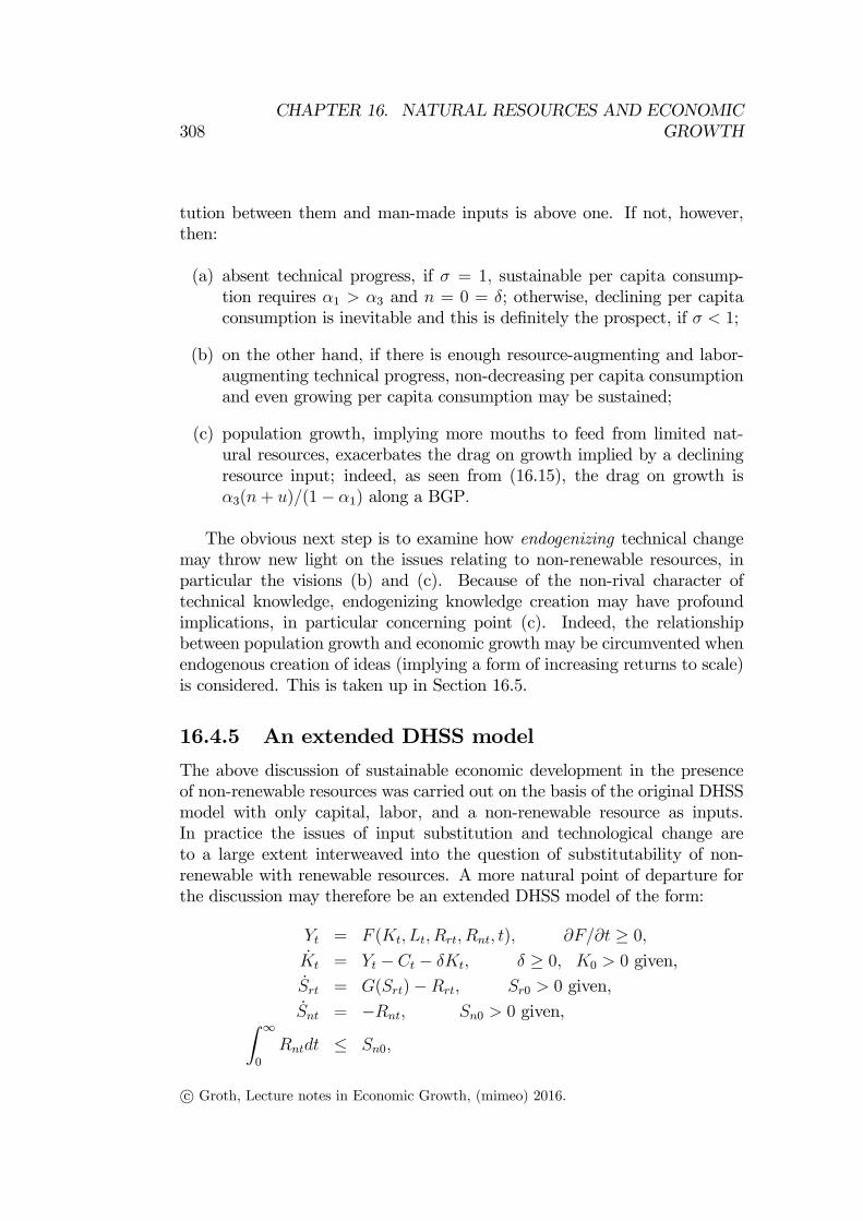
308
CHAPTER 16. NATURAL RESOURCES AND ECONOMIC
GROWTH
tution between them and man-made inputs is above one. If not, however,
then:
(a) absent technical progress, if = 1 sustainable per capita consump-
tion requires 1 3 and = 0 = ; otherwise, declining per capita
consumption is inevitable and this is definitely the prospect, if 1;
(b) on the other hand, if there is enough resource-augmenting and labor-
augmenting technical progress, non-decreasing per capita consumption
and even growing per capita consumption may be sustained;
(c) population growth, implying more mouths to feed from limited nat-
ural resources, exacerbates the drag on growth implied by a declining
resource input; indeed, as seen from (16.15), the drag on growth is
3(+ )(1− 1) along a BGP
The obvious next step is to examine how endogenizing technical change
may throw new light on the issues relating to non-renewable resources, in
particular the visions (b) and (c). Because of the non-rival character of
technical knowledge, endogenizing knowledge creation may have profound
implications, in particular concerning point (c). Indeed, the relationship
between population growth and economic growth may be circumvented when
endogenous creation of ideas (implying a form of increasing returns to scale)
is considered. This is taken up in Section 16.5.
16.4.5 An extended DHSS model
The above discussion of sustainable economic development in the presence
of non-renewable resources was carried out on the basis of the original DHSS
model with only capital, labor, and a non-renewable resource as inputs.
In practice the issues of input substitution and technological change are
to a large extent interweaved into the question of substitutability of non-
renewable with renewable resources. A more natural point of departure for
the discussion may therefore be an extended DHSS model of the form:
= ( ) ≥ 0 = − − ≥ 0 0 0 given,
= ()− 0 0 given,
= − 0 0 given,Z ∞
0
≤ 0
c° Groth, Lecture notes in Economic Growth, (mimeo) 2016.
16.5. A two-sector R&D-based model 309
where is input of the renewable resource and the corresponding stock,
while is input of the non-renewable resource to which corresponds the
stock . Only the non-renewable resource is subject to the constraint of a
finite upper bound on cumulative resource extraction.
Within such a framework a more or less gradual transition from use of
non-renewable energy forms to renewable energy forms (hydro-power, wind
energy, solar energy, biomass, and geothermal energy), likely speeded up
learning by doing as well as R&D, can be studied (see for instance Tahvonen
and Salo, 2001).
16.5 A two-sector R&D-based model
We shall look at the economy from the perspective of a fictional social plan-
ner who cares about finding a resource allocation so as to maximize the
intertemporal utility function of a representative household subject to tech-
nical feasibility as given from the initial technology and initial resources.
16.5.1 The model
In addition to cost-free resource extraction, there are two “production” sec-
tors, the manufacturing sector and the R&D sector. In the manufacturing
sector the aggregate production function is
=
0 + + + = 1 (16.16)
where is output of manufacturing goods, while , and are inputs
of capital, labor, and a non-renewable resource, respectively, per time unit
at time Total factor productivity is where the variable is assumed
proportional to the stock of technical knowledge accumulated through R&D
investment. Due to this proportionality we can simply identify with the
stock of knowledge at time .
Aggregate manufacturing output is used for consumption, investment,
in physical capital, and investment, in R&D,
+ + =
Accumulation of capital occurs according to
= − = − − − ≥ 0 0 0 given,
(16.17)
where is the (exogenous) rate of depreciation (decay) of capital.
c° Groth, Lecture notes in Economic Growth, (mimeo) 2016.
310
CHAPTER 16. NATURAL RESOURCES AND ECONOMIC
GROWTH
In the R&D sector additions to the stock of technical knowledge are cre-
ated through R&D investment, :
= − ≥ 0 0 0 given (16.18)
We allow for a positive depreciation rate, to take into account the possi-
bility that as technology advances, old knowledge becomes obsolete and then
over time gradually becomes useless in production.
Extraction of the non-renewable resource is again given by
= − ≡ − 0 0 given, (16.19)
where is the stock of the non-renewable resource (e.g., oil reserves) and
is the depletion rate. Since we must have ≥ 0 for all there is a finiteupper bound on cumulative resource extraction:Z ∞
0
≤ 0 (16.20)
Finally, population (= labor force) grows according to
= 0 ≥ 0 0 0 given.
Uncertainty is ignored and the extraction activity involves no costs.
This setup is elementarily related to what is known as “lab-equipment
models”. By investing a part of the manufacturing output, new knowledge
is directly generated without intervention by researchers and similar.15 Note
also that there are no intertemporal knowledge-spillovers.
16.5.2 Analysis
We now skip the explicit dating of the variables where not needed for clarity.
The model has three state variables, the stock, of physical capital, the
stock, of non-renewable resources, and the stock, of technical knowl-
edge. To simplify the dynamics, we will concentrate on the special case
= = In this case, as we shall see, after an initial adjustment pe-
riod, the economy behaves in many respects similarly to a reduced-form AK
model.
Let us first consider efficient paths, i.e., paths such that aggregate con-
sumption can not be increased in some time interval without being decreased
15An interpretation is that part of the activity in the manufacturing sector is directly
R&D activity using the same technology (production function) as is used in the production
of consumption goods and capital goods.
c° Groth, Lecture notes in Economic Growth, (mimeo) 2016.
16.5. A two-sector R&D-based model 311
Figure 16.3: Initial complete specialization followed by balanced growth.
in another time interval. The net marginal productivities of and are
equal if and only if − = − i.e., if and only if
=
The initial stocks, 0 and 0 are historically given. Suppose 00
as in Figure 16.3. Then, initially, the net marginal productivity of capital is
larger than that of knowledge, i.e., capital is relatively scarce. An efficient
economy will therefore for a while invest only in capital, i.e., there will be a
phase where = 0 This phase of complete specialization lasts until =
a state reached in finite time, say at time , cf. the figure. Hereafter,
there is investment in both assets so that their ratio remains equal to the
efficient ratio forever. Similarly, if initially 00 then there will
be a phase of complete specialization in R&D, and after a finite time interval
the efficient ratio = is achieved and maintained forever.
For at the aggregate level it is thus as if there were only one kind
of capital, which we may call “broad capital” and define as = +
= (+ ) Indeed, substitution of = and = (+) into
(16.16) gives
=
(+ )++ ≡ ≡ + (16.21)
c° Groth, Lecture notes in Economic Growth, (mimeo) 2016.

312
CHAPTER 16. NATURAL RESOURCES AND ECONOMIC
GROWTH
so that + + 1 Further, adding (16.18) and (16.17) gives
· = + = − − (16.22)
where is per capita consumption.
We now proceed with a model based on broad capital, using (16.21),
(16.22) and the usual resource depletion equation (16.19). Essentially, this
model amounts to an extended DHSS model allowing increasing returns to
scale, thereby offering a simple framework for studying endogenous growth
with essential non-renewable resources.
We shall focus on questions like:
1 Is sustainable development (possibly even growth) possible within the
model?
2 Can the utilitarian principle of discounted utility maximizing possibly
clash with a requirement of sustainability? If so, under what condi-
tions?
3 How can environmental policy be designed so as to enhance the prospects
of sustainable development or even sustainable economic growth?
Balanced growth
Log-differentiating (16.21) w.r.t. gives the “growth-accounting equation”
= + + (16.23)
Hence, along a BGP we get
(1− ) + = (+ − 1) (16.24)
Since 0 it follows immediately that:
Result (i) A BGP has 0 if and only if
(+ − 1) 0 or 1 (16.25)
Proof. Since 0 (*) implies (1 − ) ( + − 1) Hence, if 0 either 1 or ( ≤ 1 and ( + − 1) 0) This proves “only
if”. The “if” part is more involved but follows from Proposition 2 in Groth
(2004). ¤
c° Groth, Lecture notes in Economic Growth, (mimeo) 2016.
16.5. A two-sector R&D-based model 313
Result (i) tells us that endogenous growth is theoretically possible, if there
are either increasing returns to the capital-cum-labor input combined with
population growth or increasing returns to capital (broad capital) itself. At
least one of these conditions is required in order for capital accumulation to
offset the effects of the inescapable waning of resource use over time. Based
on Nordhaus (1992), ≈ 02 ≈ 06 ≈ 01 and ≈ 01 seem reasonable.Given these numbers,
(i) semi-endogenous growth requires (++−1) 0 hence 020;
(ii) fully endogenous growth requires + 1 hence 080
We have defined fully endogenous growth to be present if the long-run
growth rate in per capita output is positive without the support of growth in
any exogenous factor. Result (i) shows that only if 1 is fully endogenous
growth possible. Although the case 1 has potentially explosive effects
on the economy, if is not too much above 1, these effects can be held back
by the strain on the economy imposed by the declining resource input.
In some sense this is “good news”: fully endogenous steady growth is the-
oretically possible and no knife-edge assumption is needed. As we have seen
in earlier chapters, in the conventional framework without non-renewable re-
sources, fully endogenous growth requires constant returns to the producible
input(s) in the growth engine. In our one-sector model the growth engine
is the manufacturing sector itself, and without the essential non-renewable
resource, fully endogenous growth would require the knife-edge condition
= 1 ( being above 1 is excluded in this case, because it would lead to
explosive growth in a setting without some countervailing factor). When
non-renewable resources are an essential input in the growth engine, a drag
on the growth potential is imposed. To be able to offset this drag, fully
endogenous growth requires increasing returns to capital.
The “bad news” is, however, that even in combination with essential non-
renewable resources, an assumption of increasing returns to capital seems too
strong and too optimistic. A technology having just slightly above 1 can
sustain any per capita growth rate − there is no upper bound on .16 This
appears overly optimistic.
This leaves us with semi-endogenous growth as the only plausible form
of endogenous growth (as long as is not endogenous). Indeed, Result (i)
indicates that semi-endogenous growth corresponds to the case 1− ≤ 1In this case sustained positive per capita growth driven by some internal
mechanism is possible, but only if supported by 0 that is, by growth in
an exogenous factor, here population size.
16This is shown in Groth (2004).
c° Groth, Lecture notes in Economic Growth, (mimeo) 2016.

314
CHAPTER 16. NATURAL RESOURCES AND ECONOMIC
GROWTH
Growth policy and conservation
Result (i) is only about whether the technology as such allows a positive per
capita growth rate or not. What about the size of the growth rate? Can
the growth rate temporarily or perhaps permanently be affected by economic
policy? The simple growth-accounting relation (16.24) immediately shows:
Result (ii) Along a BGP, policies that decrease (increase) the depletion
rate (and only such policies) will increase (decrease) the per capita
growth rate (here we presuppose 1 the plausible case).
This observation is of particular interest in view of the fact that chang-
ing the perspective from exogenous to endogenous technical progress implies
bringing a source of numerous market failures to light. On the face of it,
the result seems to run against common sense. Does high growth not im-
ply fast depletion (high )? Indeed, the answer is affirmative, but with the
addition that exactly because of the fast depletion such high growth will
only be temporary − it carries the seeds to its own obliteration. For fastersustained growth there must be sustained slower depletion. The reason for
this is that with protracted depletion, the rate of decline in resource input
becomes smaller. Hence, so does the drag on growth caused by this decline.
As a statement about policy and long-run growth, (ii) is a surprisingly
succinct conclusion. It can be clarified in the following way. For policy to
affect long-run growth, it must affect a linear differential equation linked to
the basic goods sector in the model. In the present framework the resource
depletion relation,
= −is such an equation. In balanced growth = − ≡ − is constant,so that the proportionate rate of decline in must comply with, indeed be
equal to, that of Through the growth accounting relation (16.23), given
this fixes and (equal in balanced growth), hence also = − .
The conventional wisdom in the endogenous growth literature is that
interest income taxes impede economic growth and investment subsidies pro-
mote economic growth. Interestingly, this need not be so when non-renewable
resources are an essential input in the growth engine (which is here the man-
ufacturing sector itself). At least, starting from a Cobb-Douglas aggregate
production function as in (16.16), it can be shown that only those policies
that interfere with the depletion rate in the long run (like a profits tax on
resource-extracting companies or a time-dependent tax on resource use) can
affect long-run growth. It is noteworthy that this long-run policy result holds
whether 0 or not and whether growth is exogenous, semi-endogenous
c° Groth, Lecture notes in Economic Growth, (mimeo) 2016.

16.5. A two-sector R&D-based model 315
or fully endogenous.17 The general conclusion is that with non-renewable
resources entering the growth-generating sector in an essential way, conven-
tional policy tools receive a different role and there is a role for new tools
(affecting long-run growth through affecting the depletion rate).18
Introducing preferences
To be more specific we introduce household preferences and a social planner.
The resulting resource allocation will coincide with that of a decentralized
competitive economy if agents have perfect foresight and the government has
introduced appropriate subsidies and taxes. As in Stiglitz (1974a), let the
utilitarian social planner choose a path ( )∞=0 so as to optimize
0 =
Z ∞
0
1−
1−
− 0 (16.26)
subject to the constraints given by technology, i.e., (16.21), (16.22), and
(16.19), and initial conditions. The parameter 0 is the (absolute) elas-
ticity of marginal utility of consumption (reflecting the strength of the desire
for consumption smoothing) and is a constant rate of time preference.19
Using the Maximum Principle, the first-order conditions for this problem
lead to, first, the social planner’s Keynes-Ramsey rule,
=1
(
− − ) =
1
(
− − ) (16.27)
second, the social planner’s Hotelling rule,
()
=
(
− ) =
(
− ) (16.28)
The Keynes-Ramsey rule says: as long as the net return on investment in
capital is higher than the rate of time preference, one should let current be
low enough to allow positive net saving (investment) and thereby higher con-
sumption in the future. The Hotelling rule is a no-arbitrage condition saying
that the return (“capital gain”) on leaving the marginal unit of the resource
17This is a reminder that the distinction between fully endogenous growth and semi-
endogenous growth is not the same as the distinction between policy-dependent and policy-
invariant growth.18These aspects are further explored in Groth and Schou (2006).19For simplicity we have here ignored (as does Stiglitz) that also environmental quality
should enter the utility function.
c° Groth, Lecture notes in Economic Growth, (mimeo) 2016.

316
CHAPTER 16. NATURAL RESOURCES AND ECONOMIC
GROWTH
in the ground must equal the return on extracting and using it in produc-
tion and then investing the proceeds in the alternative asset (reproducible
capital).20
After the initial phase of complete specialization described above, we
have, due to the proportionality between and that = =
= Notice that the Hotelling rule is independent of prefer-
ences; any path that is efficient must satisfy the Hotelling rule (as well as
the exhaustion condition lim→∞ () = 0).
Using the Cobb-Douglas specification, we may rewrite the Hotelling rule
as − = − Along a BGP = = + and = − sothat the Hotelling rule combined with the Ramsey rule gives
(1− ) + = − (16.29)
This linear equation in and combined with the growth-accounting
relationship (16.24) constitutes a linear two-equation system in the growth
rate and the depletion rate. The determinant of this system is ≡ 1− −+ We assume 0 which seems realistic and is in any case necessary
(and sufficient) for stability.21 Then
=(+ + − 1)−
and (16.30)
=[(+ − 1) − ]+ (1− )
(16.31)
To ensure boundedness from above of the utility integral (16.26) we need
the parameter restriction − (1− ) which we assume satisfied for as given in (16.30).
Interesting implications are:
Result (iii) If there is impatience ( 0), then even when a non-negative
is technically feasible (i.e., (16.25) satisfied), a negative can be
optimal and stable.
20After Hotelling (1931), who considered the “rule” in a market economy. Assuming
perfect competition, the real resource price is = and the real rate of interest is
= − . Then the rule takes the form = . If there are extraction costs at
rate ( ) then the rule takes the form − = , where is the price of
the unextracted resource (whereas = + ).
It is another matter that the rise in resource prices and the predicted decline in resource
use have not yet shown up in the data (Krautkraemer 1998, Smil 2003); this may be due
to better extraction technology and discovery of new deposits. But in the long run, if
non-renewable resources are essential, this tendency inevitably will be reversed.21As argued above, 1 seems plausible. Generally, is estimated to be greater than
one (see, e.g., Attanasio and Weber 1995); hence 0 The stability result as well as
other findings reported here are documented in Groth and Schou (2002).
c° Groth, Lecture notes in Economic Growth, (mimeo) 2016.

16.5. A two-sector R&D-based model 317
Result (iv) Population growth is good for economic growth. In its absence,
when 0 we get 0 along an optimal BGP; if = 0 = 0
when = 0.
Result (v) There is never a scale effect on the growth rate.
Result (iii) reflects that utility discounting and consumption smoothing
weaken the “growth incentive”.
Result (iv) is completely contrary to the conventional (Malthusian) view
and the learning from the DHSS model. The point is that two offsetting
forces are in play. On the one hand, higher means more mouths to feed
and thus implies a drag on per capita growth (Malthus). On the other hand,
a growing labour force is exactly what is needed in order to exploit the
benefits of increasing returns to scale (anti-Malthus). And at least in the
present framework this dominates the first effect. This feature might seem
to be contradicted by the empirical finding that there is no robust correlation
between and population growth in cross-country regressions (Barro and
Sala-i-Martin 2004, Ch. 12). However, the proper unit of observation in this
context is not the individual country. Indeed, in an internationalized world
with technology diffusion a positive association between and as in (16.30)
should not be seen as a prediction about individual countries, but rather as
pertaining to larger regions, perhaps the global economy. In any event, the
second part of Result (iv) is a dismal part − in view of the projected long-runstationarity of world population (United Nations 2005).
A somewhat surprising result appears if we imagine (unrealistically) that
is sufficiently above one to make a negative number. If population
growth is absent, 0 is in fact needed for 0 along a BGP However,
0 implies instability. Hence this would be a case of an instable BGP
with fully endogenous growth.22
As to Result (v), it is noteworthy that the absence of a scale effect on
growth holds for any value of including = 123
A pertinent question is: are the above results just an artifact of the very
simplified reduced-form AK-style set-up applied here? The answer turns out
22Thus, if we do not require 0 in the first place, (iv) could be reformulated as:
existence of a stable optimal BGP with 0 requires 0. This is not to say that
reducing from positive to zero renders an otherwise stable BGP instable. Stability-
instability is governed solely by the sign of Given 0 letting decrease from a level
above the critical value, (+ + − 1) given from (16.30), to a level below, changes
from positive to negative, i.e., growth comes to an end.23More commonplace observations are that increased impatience leads to faster depletion
and lower growth (in the plausible case 1) Further, in the log-utility case ( = 1) the
depletion rate equals the effective rate of impatience, − .
c° Groth, Lecture notes in Economic Growth, (mimeo) 2016.

318
CHAPTER 16. NATURAL RESOURCES AND ECONOMIC
GROWTH
to be no. For models with a distinct research technology and intertemporal
knowledge spillovers, this is shown in Groth (2007).
16.6 Natural resources and the issue of limits
to economic growth
Two distinguished professors were asked by a journalist: Are there limits to
economic growth?
The answers received were:24
Clearly YES:
• A finite planet!• The amount of cement, oil, steel, and water that we can use is limited!Clearly NO:
• Human creativity has no bounds!• The quality of wine, TV transmission of concerts, computer games, andmedical treatment knows no limits!
An aim of this chapter has been to bring to mind that it would be strange
if there were no limits to growth. So a better question is:
What determines the limits to economic growth?
The answer suggested is that these limits are determined by the capability
of the economic system to substitute limited natural resources by man-made
goods the variety and quality of which are expanded by creation of new ideas.
In this endeavour frontier countries, first the U.K. and Europe, next the
United States, have succeeded at a high rate for two and a half century. To
what extent this will continue in the future nobody knows. Some economists,
e.g. Gordon (2012), argue there is an enduring tendency to slowing down of
innovation and economic growth (the low-hanging fruits have been taken).
Others, e.g. Brynjolfsson and McAfee (2012, 2014), disagree. They reason
that the potentials of information technology and digital communication are
on the verge of the point of ubiquity and flexible application. For these
authors the prospect is “The Second Machine Age” (the title of their recent
book), by which they mean a new innovative epoch where smart machines
and new ideas are combined and recombined - with pervasive influence on
society.
24Inspired by Sterner (2008).
c° Groth, Lecture notes in Economic Growth, (mimeo) 2016.

16.7. Bibliographic notes concerning Section 16.5 319
16.7 Bibliographic notes concerning Section
16.5
It is not always recognized that the research of the 1970s on macro implica-
tions of essential natural resources in limited supply already laid the ground-
work for a theory of endogenous and policy-dependent growth with natural
resources. Actually, by extending the DHSS model, Suzuki (1976), Robson
(1980) and Takayama (1980) studied how endogenous innovation may affect
the prospect of overcoming the finiteness of natural resources.
Suzuki’s (1976) article contains an additional model, involving a resource
externality. Interpreting the externality as a “greenhouse effect”, Sinclair
(1992, 1994) and Groth and Schou (2006) pursue this issue further. In the
latter paper a configuration somewhat similar to the model in Section 16.5 is
studied. The source of increasing returns to scale is not intentional creation
of knowledge, however, but learning as a by-product of investing as in Arrow
(1962a) and Romer (1986). Empirically, the evidence furnished by, e.g., Hall
(1990) and Caballero and Lyons (1992) suggests that there are quantitatively
significant increasing returns to scale w.r.t. capital and labour or external
effects in US and European manufacturing. Similarly, Antweiler and Trefler
(2002) examine trade data for goods-producing sectors and find evidence for
increasing returns to scale.
Concerning Result (i) in Section 16.5, note that if some irreducibly ex-
ogenous element in the technological development is allowed in the model
by replacing the constant in (16.21) by where ≥ 0, then (16.25) isreplaced by +(+− 1) 0 or 1 Both Stiglitz (1974a, p. 131) and
Withagen (1990, p. 391) ignore implicitly the possibility 1 Hence, from
the outset they preclude fully endogenous growth.
c° Groth, Lecture notes in Economic Growth, (mimeo) 2016.

320
CHAPTER 16. NATURAL RESOURCES AND ECONOMIC
GROWTH
16.8 Appendix: Balanced growth with an es-
sential non-renewable resource
The production side of the DHSS model with CES production function is
described by:
= ( ) ≥ 0 (16.32)
= − − ≥ 0 0 0 given, (16.33)
= − ≡ − 0 0 given, (16.34)
= 0 ≥ 0 (16.35)Z ∞
0
≤ 0 (16.36)
We will assume that the non-renewable resource is essential, i.e.,
= 0 implies = 0 (16.37)
From now we omit the dating of the time-dependent variables where not
needed for clarity. Recall that in the context of an essential non-renewable
resource, we define a balanced growth path (BGP for short) as a path along
which the quantities and are positive and change at constant
proportionate rates (some or all of which may be negative).
Lemma 1 Along a BGP the following holds: (a) = 0; (b) (0) =
−(0) andlim→∞
= 0 (16.38)
Proof Consider a BGP. (a) From (16.34), = −; differentiating withrespect to time gives
= −( − ) = 0
by definition of a BGP. Hence, = since 0 by definition. For any
constant we haveR∞0
=R∞0
0 If ≥ 0 (16.36) would thus be
violated. Hence, 0 (b) With = 0 in (16.34), we get 00 = −00= the last equality following from (a). Hence, 0 = −0 Finally, thesolution to (16.34) can be written = 0
Then, since is a negative
constant, → 0 for →∞ ¤Define
≡
≡
and ≡
(16.39)
We may write (16.34) as
= − − (16.40)
c° Groth, Lecture notes in Economic Growth, (mimeo) 2016.

16.8. Appendix: Balanced growth with an essential non-renewable resource321
Similarly, by (16.34),
≡ − (16.41)
Lemma 2 Along a BGP, = = − 0 is constant and = . If gross
saving is positive in some time interval, we have along the BGP in addition
that = , both constant, and that and are constant.
Proof Consider a BGP. Since is constant by definition of a BGP, must
also be constant in view of (16.41). Then, by Lemma 1, = = − isconstant and 0. Differentiating in (16.40) with respect to gives = − = ( − ) −( − ) = 0 since is constant along a BGP.
Dividing through by which is positive along a BGP, and reordering gives
− = ( − )
(16.42)
But this is a contradiction unless = ; indeed, if 6= then − 6= − at the same time as = → 0 if and
= →∞ if both cases being incompatible with (16.42) and the
presumed constancy of and hence constancy of both − and − So = along a BGP. Suppose gross saving is positive in some
time interval and that at the same time 6= = then (16.42) implies
≡ 1, i.e., = for all or gross saving = 0 for all a contradiction.
Hence, = = It follows by (16.39) that and are constant. ¤Consider the case where the production function is neoclassical with CRS,
and technical progress is labor- and resource-augmenting:
= ( 2 3) (16.43)
2 = 2, 2 ≥ 0 3 = 3 3 ≥ 0
Let ≡ 2 and ≡ 3 Let and denote the output elasticities
w.r.t. and i.e.,
≡
≡
2
(2) ≡
3
(3)
Differentiating in (16.43) w.r.t. and dividing through by (as in growth-
accounting), we then have
≡
= + (2 + ) + (3 + )
= + (2 + ) + (1− − )(3 + ) (16.44)
c° Groth, Lecture notes in Economic Growth, (mimeo) 2016.

322
CHAPTER 16. NATURAL RESOURCES AND ECONOMIC
GROWTH
the last equality being implied by the CRS property in (16.43).
Suppose the economy follows a BGP with positive gross saving. Then,
by Lemma 2, = and = − 0 Hence, (16.44) can be written
(1− )( − (3 − )) = (2 + − (3 − )) (16.45)
Consider the special case where is CES:
=³1
+ 2(2)
+ 3(3)´1
1 2 3 0X
= 1 1
(16.46)
As we know from Chapter 2 that, for = 0 the CES formula can be inter-
preted as the Cobb-Douglas formula (16.13). Applying (??) from Chapter 2,
the output elasticities w.r.t. and are
= 1
µ
¶− = 2
µ
2
¶− and = 3
µ
3
¶−
(16.47)
respectively.
Lemma 3 Let ≡ and ≡ Given (16.35) and (16.46), along a
BGP with positive gross saving, and are constant, and = = 2
In turn, such a BGP exists if and only if
= 3 − (2 + ) 0 (16.48)
Proof Consider a BGPwith positive gross saving. By Lemma 2, 0 = −is constant and ≡ is constant, hence so is The left hand side of
(16.45) is thus constant and somust the right-hand side therefore be. Suppose
that, contrary to (16.48), 6= 3−(2+). Then constancy of the right-handof (16.45) requires that is constant. In turn, by (16.47), this requires that
(2) ≡ 2 is constant. Consequently, = 2 = where the second
equality is implied by the claim in Lemma 2 that along a BGP with positive
gross saving in some time interval, = As is constant, it follows
that = ≡ + = 2+ Inserting this into (16.44) and rearranging,
we get
(1− − )(2 + ) = (1− − )(3 − )
where the last equality follows from = −. Isolating gives the equalityin (16.48). Thereby, our assumption 6= 3 − (2 + ) leads to a contradic-
tion. Hence, given (16.35) and (16.46), if a BGP with positive gross saving
exists, then = 3 − (2 + ) 0. This shows the necessity of (16.48).
The sufficiency of (16.48) follows by construction, starting by fixing and
thereby − in accordance with (16.48) and moving “backward”, showingconsistency with (16.44) for = = 2 + . ¤
c° Groth, Lecture notes in Economic Growth, (mimeo) 2016.
16.9. References 323
16.9 References
Antràs, 2004, ...
Arrow, K. J., 1962, The economic implications of learning by doing, Review
of Economic Studies 29, 153-73.
Arrow, K. J., P. Dasgupta, L. Goulder, G. Daily, P. Ehrlich, G. Heal, S.
Levin, K.-G. Mäler, S. Schneider, D. Starrett, and B. Walker, 2004,
Are we consuming too much?, J. of Economic Perspectives 18, no. 3,
147-172.
Arrow, K.J, P. Dasgupta, L. Goulder, K. Mumford, and K.L.L. Oleson,
2012, Sustainability and the measurement of wealth, Environment and
Development Economics 17, no. 3, 317—353.
Barro, R., and X. Sala-i-Martin, 2004, .....
Brock, W. A., and M. Scott Taylor, 2005. Economic Growth and the Envi-
ronment: A review of Theory and Empirics. In: Handbook of Economic
Growth, vol. 1.B, ed. by ...
Brock, W. A., and M. Scott Taylor, 2010, , J. of Economic Growth, vol.
Brundtland Commission, 1987, ...
Brynjolfsson, E., and A. McAfee, 2014, The Second Machine Age, Norton.
Caballero, R. J., and R. K. Lyons, The case of external economies. In:
Political Economy, Growth, and Business Cycles, ed. by A. Cukierman,
Z. Hercowitz and L. Leiderman, MIT Press, Cambridge, MA, 1992, pp.
117-139.
Dasgupta, P., 1993, Natural resources in an age of substitutability. In:
Handbook of Natural Resource and Energy Economics, vol. 3, ed. by
A. V. Kneese and J. L. Sweeney, Elsevier: Amsterdam, 1111-1130.
Dasgupta, P., and G. M. Heal, 1974, The optimal depletion of exhaustible
resources, Review of Economic Studies, vol. 41, Symposium, 3-28.
Dasgupta, P., and G. M. Heal, 1979, Economic Theory and Exhaustible
Resources, Cambridge University Press, Cambridge.
c° Groth, Lecture notes in Economic Growth, (mimeo) 2016.

324
CHAPTER 16. NATURAL RESOURCES AND ECONOMIC
GROWTH
Dasgupta, P., G. M. Heal and M. K. Majumdar, 1977, Resource deple-
tion and research and development. In: Frontiers of Quantitative Eco-
nomics, vol. IIIB, ed. by M. D. Intrilligator, North-Holland, Amster-
dam, 483-505.
Dasgupta, P., G. M. Heal and A. K. Pand, 1980, Funding research and
development, Applied Mathematical Modeling 4, 87-94.
Fagnart, J.-F., and M. Germain, 2011, Quantitative vs. qualitative growth
with recyclable resources, Ecological Economics, vol. 70, 929-941.
Gordon, R.J., 2012, Is US economic growth over? Faltering innovation
confronts the six headwinds, NBER WP no. 18315.
Grimaud, A., and L. Rougé, 2003, Non-renewable resources and growth
with vertical innovations: optimum, equilibrium and economic policies,
Journal of Environmental Economics and Management 45, 433-453.
Grossman, G.M., and A.B. Krueger, 1995, , QJE, vol. 90 (2).
Groth, C., 2004, Strictly endogenous growth with non-renewable resources
implies an unbounded growth rate, Topics in Macroeconomics 4 (1),
1-13.
Groth, C., 2007, A New-Growth Perspective on Non-renewable Resources.
In: Sustainable Resource Use and Economic Dynamics, ed. by L.
Bretschger and S. Smulders, Springer Verlag: Dordrecht (available at
the course website).
Groth, C., and P. Schou, 2002, Can nonrenewable resources alleviate the
knife-edge character of endogenous growth? Oxford Economic Papers
54, 386-411.
−− , 2006, Growth and non-renewable resources: The different roles of
capital and resource taxes, Journal of Environmental Economics and
Management, forthcoming.
Hall, R. E., 1990, Invariance properties of Solow’s residual. In: Growth/Productivity/Un-
employment. Essays to Celebrate Bob Solow’s Birthday, ed. by P.
Diamond, MIT Press, Cambridge (Mass.), 71-112.
Hamilton, K., 2012, Comments on Arrow et al., ‘Sustainability and the
measurement of wealth’, Environment and Development Economics 17,
no. 3, 356 - 361.
c° Groth, Lecture notes in Economic Growth, (mimeo) 2016.
16.9. References 325
Handbook of Natural Resource and Energy Economics, vol. III, ed. by A.
V. Kneese and J. L. Sweeney, Elsevier: Amsterdam, 1993.
Hartwick, J. M., 1977, Intergenerational equity and the investing of rents
from exhaustible resources, American Economic Review 67, 972-974.
Heal, G., 1998. Valuing the Future. Economic Theory and Sustainability.
Columbia University Press: New York.
Hotelling, H., 1931, The economics of exhaustible resources, Journal of Po-
litical Economy 39, 137-175.
Jones, C., 2002, Introduction to Economic Growth, 2. ed., W.W. Norton:
New York.
Kamien, M. I., and N. L. Schwartz, 1978, Optimal exhaustible resource de-
pletion with endogenous technical change, Review of Economic Studies
45 (1), 179-196.
Krautkraemer, J., 1985, Optimal growth, resource amenities and the preser-
vation of natural environments, Review of Economic Studies 52, 153-
170.
−− , 1998, Nonrenewable resource scarcity, Journal of Economic Literature36 (4), 2065-2107.
Lind, S., og P. Schou, P., 2013, Ægte opsparing, Arbejdspapir 2013:1, De
Økonomiske Råds Sekretariat, København.
Meadows, D. H., D. Meadows, J. Randers, and W. W. Behrens III, 1972,
The Limits to Growth, Universe Books: New York.
Meadows, D. H., D. L. Meadows and J. Randers, 1992, Beyond the Limits,
Chelsea Green Publ. Com., Post Mills.
Meadows, D. H., D. Meadows, and J. Randers, 2004, Limits to Growth: The
30-Year Update,...
Neumayer, E., 2000, Scarce or abundant? The economics of natural resource
availability, Journal of Economic Surveys 14 (3), 307-335.
Nordhaus, W., 1969, An economic theory of technological change, American
Economic Review 59 (2), 18-28.
Nordhaus, W. , 1992, Lethal Model 2: The limits to growth revisited, Brook-
ings Papers on Economic Activities, (2), 1-43.
c° Groth, Lecture notes in Economic Growth, (mimeo) 2016.

326
CHAPTER 16. NATURAL RESOURCES AND ECONOMIC
GROWTH
Nordhaus, W.D., 1999, Quality change in price indices, J. of Economic
Perspectives, vol. 12 (1), 59-68.
Nordhaus, W., and J. Tobin, 1972, Is growth obsolete? In: Economic
Growth: Fiftieth Anniversary ColloquiumV, Columbia University Press,
New York. Reprinted in: J. Tobin, Essays in Economics. Theory and
Policy, The MIT Press, Cambridge (Mass.) 1985, 360-450.
Popp, D., 2002, Induced innovation and energy prices, American Economic
Review 92 (1), 160-180.
Robson, A. J., 1980, Costly innovation and natural resources, International
Economic Review 21, 17-30.
Schou, P., 2000, Polluting nonrenewable resources and growth, Environ-
mental and Resource Economics 16, 211-27.
−− , 2002, When environmental policy is superfluous: Growth and pollutingresources, Scandinavian Journal of Economics 104, 605-620.
Seierstad, A., and K. Sydsaeter, 1987, Optimal Control Theory with Eco-
nomic Applications, North Holland, Amsterdam.
Sinclair, P., 1994, On the optimum trend of fossil fuel taxation, Oxford
Economic Papers 46, 869-877.
Smil, V., 2003, Energy at the crossroads. Global perspectives and uncertain-
ties, Cambridge Mass.: MIT Press.
Smulders, S., 1995, Entropy, environment, and endogenous growth, Inter-
national Tax and Public Finance, vol. 2, 319-340.
Smulders, S., 1999,...
Smulders, S., 2012, An arrow in the Achilles’ heel of sustainability and
wealth accounting, Environment and Development Economics 17, no.
3, 368-372.
Smulders, S., and M. de Nooij, 2003, The impact of energy conservation on
technology and economic growth, Resource and Energy Economics 25,
59-79.
Solow, R.M., 1973, Is the end of the world at hand? Challenge, vol. 16, no.
1, 39-50.
c° Groth, Lecture notes in Economic Growth, (mimeo) 2016.

16.9. References 327
Solow, R. M., 1974a, Intergenerational equity and exhaustible resources,
Review of Economic Studies 41, Symposium Issue, 29-45.
−− , 1974b, The economics of resources or the resources of economics,
American Economic Review 64, Papers and Proceedings, 1-14.
Solow, R.M., 2012, A few comments on ‘Sustainability and the measurement
of wealth, Environment and Development Economics 17, no. 3, 354-
355.
Squires and Vestergaard, 2011,
Sterner, T., 2008, The costs and benefits of climate policy: The impact of
the discount rate and changing relative prices. Lecture at Miljøøkonomisk
konference 2008 in Skodsborg, see http://www.dors.dk/graphics/Synkron-
Library/Konference%202008/
Keynote/Sterner_Copenhagen_SEPT08.pdf
Stiglitz, J., 1974a, Growth with exhaustible natural resources: Efficient and
optimal growth paths, Review of Economic Studies 41, Symposium
Issue, 123-137.
−− , 1974b, Growth with exhaustible natural resources: The competitiveeconomy, Review of Economic Studies 41, Symposium Issue, 139-52.
Stiglitz, J., A. Sen, and J.-P. Fitoussi, 2009, Report by the Commission
on the Measurement of Economic Performance and Social Progress,
www.stiglitz-sen-fitoussi.fr.
Stiglitz, J., A. Sen, and J.-P. Fitoussi, 2010, Mismeasuring Our Lives. Why
the GDP Doesn’t Add Up, The New Press: New York.
Suzuki, H., 1976, On the possibility of steadily growing per capita consump-
tion in an economy with a wasting and non-replenishable resource, Re-
view of Economic Studies 43, 527-35.
Tahvonen, O., and S. Salo, 2001, Economic growth and transitions between
renewable and nonrenewable energy resources, European Economic Re-
view 45, 1379-1398.
Takayama, A., 1980, Optimal technical progress with exhaustible resources.
In: Exhaustible Resources, Optimality, and Trade, ed. by M. C. Kemp
and N. V. Long, North-Holland, Amsterdam, 95-110.
c° Groth, Lecture notes in Economic Growth, (mimeo) 2016.

328
CHAPTER 16. NATURAL RESOURCES AND ECONOMIC
GROWTH
United Nations, 2005, World Population Prospects. The 2004 Revision,
Population Division, New York.
van Kooten, G. C., and E. H. Bulte, 2000. The Economics of Nature.
Managing Biological Assets. Blackwell: Oxford.
Weitzman, M., 2001, A contribution to the theory of welfare accounting,
Scandinavian J. of Economics 103 (1), 1-23.
Weitzman, M., 2003, Income, Wealth, and the Maximum Principle, Harvard
Univ. Press: Cambridge (Mass.).
Withagen, C., 1990, Topics in resource economics. In: Advanced Lectures
in Quantitative Economics, ed. by F. van der Ploeg, Academic Press,
London, 381-419.
c° Groth, Lecture notes in Economic Growth, (mimeo) 2016.

Short Note 1. Economic Growth.
April 11, 2016. Christian Groth
Robustness issues and scale effects
This note adds some conceptual and empirical perspectives to the discussion in Chap-
ter 5 and 9 in Jones and Vollrath (2013).
1 Different growth patterns
Notation: Y = GDP, y ≡ Y/L, and gy ≡ y/y; time is continuous.
Economic growth can take different forms. It can be exponential :
yt = y0egt, g > 0. (1)
Ignoring business cycle fluctuations this describes quite well what we have seen in indus-
trialized economies since the industrial revolution (with g ∈ (0.01, 0.02) on annual basis).When growth is exponential, the growth rate, y/y, is a positive constant, here equal to g.
Growth can alternatively take the form of arithmetic growth:
yt = y0 + αt, α > 0. (2)
Here y = α, the momentum, is a positive constant. So, in spite of the growth rate, y/y,
approaching zero for t going to infinity, we have yt →∞ for t→∞.
More generally, growth can take the form of quasi-arithmetic growth:
yt = y0(1 + αβt)1/β, α > 0, β > 0. (3)
In the special case β = 1 and y0 = 1, this is arithmetic growth. The parameter β is the
damping coeffi cient. The case of strict stagnation, yt = y0 for all t ≥ 0, can be interpretedas the limiting case β →∞.1 On the other hand, in the limit, when β → 0 (no damping),
the growth path (3) becomes exponential growth, yt = y0eαt.2
1To see this, use L’Hôpital’s rule for “∞/∞”on ln yt = ln y0 + 1β ln (1 + αβt). The term stagnation
also covers the case of asymptotic stagnation where in spite of y > 0 for all t ≥ 0, y goes towards zerofast enough so that there is an upper bound, y, for yt, i.e., yt < y for all t ≥ 0. For instance logisticgrowth has this property. (Logistic growth is the growth path generated by the differential equation yt= αyt(1− yt/y), α > 0, 0 < y0 < y.)
2To see this, use L’Hôpital’s rule for “0/0”on ln yt = ln y0 + 1β ln (1 + αβt).
1

These alternative growth patterns can be generated for alternative parameter values
of essentially the same model, namely a model that leads to the differential equation
yt = αyβ0 yt1−β, α > 0, β ≥ 0. (4)
In case β = 0, (4) is a linear differential equation that has the solution (1) with g = α,
which is exponential growth. In case β > 0, (4) is an autonomous Bernoulli equation that
has the solution (3), which is quasi-arithmetic growth.3 For alternative values of β between
0 and infinity, quasi-arithmetic growth covers the whole range between exponential growth
and strict stagnation. We rule out the case of β < 0 which would imply that the model
could only temporarily describe reality, because β < 0 leads to explosive growth: yt
approaching infinity in finite time (the “end of scarcity”).
Several prominent macroeconomists, e.g., Lawrence Summers, Robert Gordon, and our
own Charles Jones, predict that economic growth in the future will be lower than what
we have seen in the 20th century. One of the reasons emphasized by Jones and others
is the slowdown of population growth and thereby, everything else equal, dampening of
growth of the source of new ideas. Along this line, in a coming exercise you will be asked
to show what long-run growth pattern the horizontal innovations model with ϕ < 1 and
n = 0 implies.
2 The term “endogenous growth”and all that
How terms like “endogenous growth”and “semi-endogenous growth”are defined varies
in the literature. In this course we use the following definitions. A model features:
endogenous growth if yt →∞ for→∞, and the source of this evolution is some internalmechanism in the model (rather than exogenous technology growth);
fully-endogenous growth if growth is endogenous in such way that yt → ∞ for → ∞occurs even if there is no support by growth in any exogenous factor;4
3It is clear that with 0 < β < ∞, the solution formula (3) can not be extended, without bound,backward in time. For t = −(αβ)−1 ≡ t, we get yt = 0, and thus, according to (4), yt = 0 for allt ≤ t. This should not, however, be considered a necessarily problematic feature. A certain growthregularity need not be applicable to all periods in history. It may apply only to specific historical epochscharacterized by a particular institutional environment.
4An alternative name for this case is strictly endogenous growth.
2

semi-endogenous growth if growth is endogenous in such way that yt → ∞ for → ∞occurs only if the growth path is supported by growth in some exogenous factor
(for example exogenous growth in the labor force).
If in the above three cases, the weak growth criterion “yt →∞ for→∞”is replaced byexponential growth, then we speak of endogenous, fully-endogenous, and semi-endogenous
exponential growth, respectively. If instead the weak growth criterion is replaced by,
for instance, arithmetic growth, we speak of endogenous, fully-endogenous, and semi-
endogenous arithmetic growth, respectively,
An example of fully endogenous exponential growth is the endogenous growth gener-
ated in the Romer case (ϕ = 1, n = 0) of the horizontal innovations model. An example
of semi-endogenous exponential growth is the Jones case (ϕ < 1, n > 0) of the horizontal
innovations model.
When Romer’s case is combined with Ramsey households, we get steady-state results
of the following kind: ∂g∗y/∂ρ < 0 and ∂g∗y/∂θ < 0 (standard notation). That is, preference
parameters matter for long-run growth. This suggests, at least at the theoretical level,
that taxes and subsidies, by affecting incentives, may have effects on long-run growth.
In any case, fully-endogenous exponential growth is technologically possible if and only
if there are non-diminishing returns (at least asymptotically) to the producible inputs in
the growth-generating sector(s), also called the growth engine. The growth engine in an
endogenous growth model is defined as the set of input-producing sectors or activities
using their own output as input. This set may consist of only one element, for instance
the R&D sector in the horizontal innovations model, the manufacturing sector in the
simple AK model, and the educational sector in the Lucas (1988) model. A model is
capable of generating fully-endogenous exponential growth if the growth engine has CRS
w.r.t. producible inputs.
No argument, however, like the replication argument for CRS w.r.t. the rival inputs ex-
ists regarding CRS w.r.t. the producible inputs. This theoretical limitation, combined with
strong empirically founded skepticism, motivated Jones to introduce his semi-endogenous
version of the horizontal innovations model (Jones1995a, 1995b), where ϕ < 1, n > 0. In
that version, in the long run
gy = gk = gc =n
1− ϕ ≡ g∗y. (5)
3

If a certain degree, ξ, of R&D overlap is added, 0 ≤ ξ < 1, we instead get g∗y = (1 −ξ)n/(1− ϕ).5
So, in this case, if and only if n > 0, can a positive constant per capita growth rate be
maintained forever. Only when the R&D outcome is assisted by growth in the exogenous
source of ideas, population, is the growth engine strong enough to maintain exponential
growth. The key role of population growth derives from the fact that at the aggregate
level there are increasing returns to scale w.r.t. capital, labor, and knowledge. For the
increasing returns to be suffi ciently exploited to generate exponential growth, population
growth is needed. Note that if the Jones case is combined with Ramsey households, we
get ∂g∗y/∂ρ = 0 = ∂g∗y/∂θ, that is, preference parameters do not matter for long-run
growth (only for the level of the growth path, see Section 4 below). This suggests that
taxes and subsidies do not have long-run growth effects. Yet, in the Jones model and
similar semi-endogenous growth models, economic policy can have important permanent
level effects. Moreover, the only temporary growth effects can be quite durable because
the speed of convergence is low (see Jones, 1995a).
Strangely enough, some textbooks (for example Barro and Sala-i-Martin, 2004) do
not call much attention to the distinction between fully-endogenous growth and semi-
endogenous growth (and even less attention to the distinction between exponential growth
and weaker forms of growth). Rather, they tend to use the term “endogenous growth”
as synonymous with what we here call “fully-endogenous exponential growth”. But there
is certainly no reason to rule out apriori the parameter cases corresponding to semi-
endogenous growth.
In the Acemoglu textbook (Acemoglu, 2009, p. 448), “semi-endogenous growth” is
defined or characterized as endogenous growth where the long-run per capita growth
rate of the economy “does not respond to taxes or other policies”. As an implication,
endogenous growth which is not semi-endogenous is in Acemoglu’s text implicitly defined
as endogenous growth where the long-run per capita growth rate of the economy does
respond to taxes or other policies.
We have defined the distinction between “semi-endogenous growth”and “fully-endogenous
growth” in a different way. In our terminology, this distinction does not coincide with
the distinction between policy-dependent and policy-invariant growth. Indeed, in our ter-
5Of course the model shifts from featuring “semi-”to featuring “fully-endogenous”exponential growthif the model is extended with an internal mechanism determining the population growth rate. Jones (2003)takes steps towards such a model.
4

minology positive per capita growth may rest on an “exogenous source” in the sense of
deriving from exogenous technical progress and yet the long-run per capita growth rate
may be policy-dependent. In Chapter 16 of the lecture notes we will see an example in
connection with the Dasgupta-Heal-Solow-Stiglitz model, also known as the DHSS model.
There also exist models that according to our definition feature semi-endogenous
growth and yet the long-run per capita growth rate is policy-dependent (Cozzi, 1997;
Sorger, 2010). Similarly, there exist models that according to our definition feature fully-
endogenous exponential growth and yet the long-run per capita growth rate is policy-
invariant (some learning-by-doing models have this property).
Before proceeding, a word of warning. The distinction between “exogenous” and
“endogenous” growth is only meaningful within a given meta-theoretical framework. It
is always possible to make the meta-theoretical framework so broad that the per capita
growth rate must be considered endogenous within that framework. From the perspective
of society as a whole we can imagine many different political and institutional structures−as witnessed by long-run historical evolution − some of which clearly are less conducive toeconomic growth than others. From this broad point of view, growth is always endogenous.
3 Robustness of endogenous growth models
The horizontal innovations model illustrates the fact that endogenous growth models with
exogenous population typically exist in two varieties or cases. One is the fully-endogenous
growth case where a particular value is imposed on a key parameter in the growth engine.
This value is such that there are constant returns (at least asymptotically) to producible
inputs in the growth engine of the economy. In the “corresponding” semi-endogenous
growth case, the key parameter is allowed to take any value in an open interval. The
endpoint of this interval appears as the “knife-edge”value assumed in the fully-endogenous
growth case.
Although the two varieties build on qualitatively the same mathematical model of a
certain growth mechanism (say, research and development or learning by doing, to be
considered later in the course), the long-run results turn out to be very sensitive to which
of the two cases is assumed. In the fully-endogenous growth case a positive per-capita
growth rate is maintained forever without support of growth in any exogenous factor. In
the semi-endogenous growth case, the growth process needs “support”by some growing
5

exogenous factor in order for sustained growth to be possible. The established terminology
is somewhat seductive here. “Fully endogenous”sounds as something going much deeper
than “semi-endogenous”. But nothing of that sort should be implied. It is just a matter
of different parameter values.
As Solow (1997, pp. 7-8) emphasizes in connection with learning-by-investing models
(with constant population), the knife-edge case assumed in the fully-endogenous growth
versions is a very special case, indeed an “extreme case, not something intermediate”.
A value slightly above the knife-edge value leads to explosive growth: infinite output in
finite time even when n = 0. And a value slightly below the knife-edge value leads to
growth petering out in the long run when n = 0.
Whereas the strength of the semi-endogenous growth case is its theoretical and empir-
ical robustness, the convenience of the fully-endogenous growth case is that it has much
simpler dynamics. Then the question arises to what extent a fully-endogenous growth
model can be seen as a useful approximation to its semi-endogenous growth “counter-
part”. Imagine that we contemplate applying the fully-endogenous growth case as a basis
for making forecasts or for policy evaluation in a situation where the “true”case is the
semi-endogenous growth case. Then we would like to know: Are the impulse-response
functions generated by a shock in the fully-endogenous growth case an acceptable ap-
proximation to those generated by the same shock in the corresponding semi-endogenous
growth case for a suffi ciently long time horizon to be of interest?6 The answer is “yes”
if the critical parameter has a value “close”to the knife edge value and “no”otherwise.
How close it need be, depends on circumstances. My own tentative impression is that
usually it is “closer”than what the empirical evidence warrants.
Even if a single growth-generating mechanism, like learning by doing, does not in
itself seem strong enough to generate a reduced-form AK model (the fully-endogenous
growth case), there might exist complementary factors and mechanisms that in total
could generate something close to a reduced-form AK model. The time-series test by, for
instance, Jones (1995b) and Romero-Avila (2006), however, reject this.7
Comment on “growth petering out”when n = 0 The above-mentioned “petering
out”of long-run growth in the semi-endogenous case when n = 0 takes different forms in
6Obviously, the ultimate effects of the shock tend to be very different in the two models.7For an opposite view, see Kocherlakota and Yi (1997). There is a longstanding discussion about
these time-series econometric issues. See the course website under Supplementary Material.
6
different models. When exponential growth cannot be sustained in a model, sometimes
it remains true that nevertheless y → ∞ for t → ∞, for instance in the form of quasi-
arithmetic growth, and sometimes instead asymptotic stagnation results.8
Another issue is whether there exist factors that in spite of n = 0 (or, to be more
precise, in spite of n decreasing, possibly to zero as projected by the United Nations
(2013) to happen within a century from now) may replace the growth-supporting role
of population growth under semi-endogenous parameter conditions like ϕ < 1. Both
urbanization and the evolution of digital information and communication technologies
seem likely for a long time to at least help in that direction.
4 Weak and strong scale effects
The distinction between weak and strong scale effects is important. In the Romer case
(ϕ = 1, n = 0) of the horizontal innovations model there a strong scale effect:
∂g∗y∂L
> 0. (6)
Interpreting the size (“scale”) of the economy as measured by the size, L, of the labor
force, we call such an effect a strong scale effect, that is, “scale” has an effect on the
long-run growth rate. This kind of scale effect has clearly been rejected by the empirics,
cf. Jones and Vollrath (2013, p. 106).
Scale effects can be of a less dramatic form. In this case we speak of a weak scale effect
or a scale effect on levels. This form arises when ϕ is less than 1. We see from (5) that
in the Jones case (ϕ < 1, n > 0) of the horizontal innovations model, the steady state
growth rate is independent of the size of the economy. Consequently, in Jones’version
there is no strong scale effect. Yet there is a scale effect on levels unless ϕ = 0. If ϕ > 0,
the scale effect is positive in the sense that along a steady state growth path, (y∗t )∞t=0,
∂y∗t∂L0
> 0, (7)
cf. Exercise VII.7.
The result (7) says the following. Suppose we consider two closed economies charac-
terized by the same parameters, including the same n > 0 and the same ϕ ∈ (0, 1). Theeconomies differ only w.r.t. initial size of the labor force. Suppose both economies are
8See Groth et al., 2010.
7

in steady state. Then, according to (7), the economy with the larger labor force has, for
all t, larger output per unit of labor. The background is the increasing returns to scale
w.r.t. capital, labor, and technical knowledge, which in turn is due to technical knowl-
edge being a non-rival good − its use by one firm does not (in itself) limit the amount
of knowledge available to other firms.9 In a large economic system, say an integrated
set of open economies, more people benefit from a given increase in knowledge than in a
small economic system. At the same time the per capita cost of creating the increase in
knowledge is less in the large system than in the small system.
The scale effect on levels displayed by (7) can be shown to be increasing in the para-
meter ϕ, which measures the elasticity of the economy-wide R&D productivity w.r.t. the
stock of knowledge. When ϕ → 1, the scale effect becomes more and more powerful. In
the limit it ends up as a scale effect on the growth rate, as in the Romer case.
5 Discussion
Are there good theoretical and/or empirical reasons to believe in the existence of (positive)
scale effects on levels or perhaps even on growth in the long run?
Let us start with some theoretical considerations.
5.1 Theoretical aspects
From the point of view of theory, we should recognize the likelihood that offsetting forces
are in play. On the one hand, there is the problem of limited natural resources. For
a given level of technology, if there are CRS w.r.t. capital, labor, and land (or other
natural resources), there are diminishing returns to capital and labor taken together. In
this Malthusian perspective, an increased scale (increased population) results, everything
else equal, in lower rather than higher per capita output, that is, a negative scale effect
should be expected.
On the other hand, there is the anti-Mathusian view that repeated improvements
in technology tend to overcome, or rather more than overcome, this Malthusian force,
if appropriate socio-economic conditions are present. Here the theory of endogenous
technical change comes in by telling us that a large population may be good for technical
9By patent protection, secrecy, and copyright some aspects of technical knowledge are sometimespartially and temporarily excludable, but that is another matter.
8

progress if the institutions in society are growth-friendly. A larger population breeds
more ideas, the more so the better its education is; a larger population also promotes
division of labor and larger markets. This helps the creation of new technologies or,
from the perspective of an open economy, it helps the local adoption of already existing
technologies outside the country. In a less spectacular way it helps by furthering day-
by-day productivity increases due to learning by doing and learning by watching. The
non-rival character of technical knowledge is an important feature behind all this. It
implies that output per capita depends on the total stock of ideas, not on the stock per
person. This implies − everything else equal − an advantage of scale.
In the models considered so far in this course, natural resources and the environment
have been more or less ignored. Here only a few remarks about this limitation. The
approach we have followed is intended to clarify certain mechanisms − in abstraction
from numerous things. The models in focus have primarily been about aspects of an
industrialized economy. Yet the natural environment is always a precondition. A ten-
dency to positive scale effects on levels may be more or less counteracted by congestion
and aggravated environmental problems ultimately caused by increased population and a
population density above some threshold.
What can we say from an empirical point of view?
5.2 Empirical aspects
First of all we should remember that in view of cross-border diffusion of ideas and tech-
nology, a positive scale effect (whether weak or strong) should not be seen as a prediction
about individual countries, but rather as pertaining to larger regions, nowadays probably
the total industrialized part of the world. So cross-country regression analysis is not the
right framework for testing for scale effects, whether on levels or the growth rate. The
relevant scale variable is not the size of the country, but the size of a larger region to which
the country belongs, perhaps the whole world; and multivariate time series analysis seems
the most relevant approach.
Since in the last century there has been no clear upward trend in per capita growth
rates in spite of a growing world population (and also a growing population in the in-
dustrialized part of the world separately), most economists do not believe in strong scale
effects. But on the issue of weak scale effects the opinion is definitely more divided.
Considering the very-long run history of population and per capita income of different
9

regions of the world, there clearly exists evidence in favour of scale effects (Kremer, 1993).
Whether advantages of scale are present also in a contemporary context is more debated.
Recent econometric studies supporting the hypothesis of positive scale effects on levels
include Antweiler and Trefler (2002) and Alcalá and Ciccone (2004). Finally, considering
the economic growth in China and India since the 1980s, we must acknowledge that this
impressive performance at least does not speak against the existence of positive scale
effects on levels.
Acemoglu seems to find positive scale effects on levels plausible at the theoretical level
(pp. 113-114). At the same time, however, later in his book he seems somewhat skeptical
as to the existence of empirical support for this. Indeed, with regard to the fact that R&D-
based theoretical growth models tend to generate at least weak scale effects, Acemoglu
claims: “It is not clear whether data support these types of scale effects” (Acemoglu,
2009, p. 448).
My personal view on the matter is that we should, of course, recognize that offsetting
forces, coming from our finite natural environment, are in play and that a lot of uncertainty
is involved. Nevertheless it seems likely that at least up to a certain point there are positive
scale effects on levels.
5.3 Policy implications
If this holds true, it supports the view that international economic integration is generally
a good idea. The concern about congestion and environmental problems, in particular
global warming, should probably, however, preclude recommending governments and the
United Nations to try to promote population growth.
Moreover, it is important to remember the distinction between the global and the
local level. The n in the formula (5) refers to a much larger region than a single country;
we may refer to this region as “the set of knowledge-producing countries in the world”.
No recommendation of higher population growth in a single country is implied by this
theoretical formula. When discussing economic policy from the perspective of a single
country, all aspects of relevance in the given local context should be incorporated. For
a developing country with limited infrastructure and weak educational system, family-
planning programs and similar may in many cases make sense from both a social and a
productivity point of view (cf. Dasgupta, 1995).
10
6 References
Antweiler and Trefler, 2002, , AER.
Alcalá and Ciccone, 2004, , QJE.
Arrow, K. J., 1962. The Economic Implications of Learning by Doing. Review of Eco-
nomic Studies 29, 153-73.
Cozzi, 1997, , Journal of Economic Growth.
Gordon, R. J., 2003.
Groth, C., T. M. Steger, and K.-J. Koch, 2010. When economic growth is less than
exponential, Economic Theory 44, 213-242.
Ha, J., and P. Howitt, 2007, Accounting for trends in productivity and R&D: A Schum-
peterian critique of semi-endogenous growth theory, Journal of Money, Credit, and
Banking, vol. 39, no. 4, 733-774.
Jones, C. I., 1995a, R&D-based models of economic growth, Journal of Political Econ-
omy.
Jones, C. I., 1995b. Time series tests of endogenous growth models. Quarterly Journal
of Economics, 110 (2), 495-525.
Jones, C. I., 1999, Growth: With or without scale effects , American Economic Review,
vol. 89, Papers and proceedings, May, 139-144.
Jones, C. I., 2003, Population and ideas: A theory of endogenous growth,. In: ...
Jones, C. I., 2005. Growth and ideas. In: Handbook of Economic Growth, vol. 1B, ed.
by P. Aghion and S. N. Durlauf, Elsevier: Amsterdam, 1063-1111.
Kocherlakota and Yi, 1997.
Kremer, M., 1993, , QJE.
Lucas, R. Jr., 1988.
Razin, A., and E. Sadka, 1995, Population Economics, MIT Press.
Romer, P., 1990,
11

Romero-Avila, D., 2006, Can the AK model be rescued? New evidence from unit root
tests with good size and power, Topics in Macroeconomics, vol. 6 (1), Article 3.
Solow, R. M., 1994, ....., J. Econ. Perspectives.
Solow. R. M., 1997, Learning from ‘Learning by Doing’, Stanford.
Sorger, G., 2010, , Economica.
–
12

Short Note 2. Economic Growth.
May 6, 2016. Christian Groth
The Romer-Jones horizontalinnovations model
Below is a compact version of the Romer-Jones model of horizontal innovations in a
closed industrialized economy. In contrast to Jones and Vollrath, Ch. 5.1-2, we specify
the household sector to be of Ramsey type. There is no uncertainty and households have
perfect foresight. The text is not meant to be a substitute to Jones and Vollrath’s Ch.
5.1-2, but a complement to be read after Jones and Vollrath’s introduction has been read.
The aim is to give a systematic overview and to clarify some of the more technical issues.
Our notation is as in exercises VII.10 - VII.14, thereby only in a few respects deviating
from that in Jones and Vollrath.
1 The household sector
There is a fixed number of infinitely-lived households, all alike. Each household has L(t)
= L(0)ent members, n ≥ 0, and each member supplies inelastically one unit of labor per
time unit. We normalize the number of households to be one. Given θ > 0 and ρ > 0,
the representative household’s problem is to choose a plan (c(t))∞t=0 so as to
max U0 =
∫ ∞0
c(t)1−θ
1− θ e−(ρ−n)tdt s.t. (*)
c(t) ≥ 0,
a(t) = (r(t)− n)a(t) + w(t)− c(t), a(0) given,
limt→∞
a(t)e−∫ t0 (r(s)−n)ds ≥ 0. (NPG)
Here r(t) is the risk-free interest rate, and a(t) is per capita financial wealth, which can
be placed in “raw capital”or perpetual patents, as described below.
The solution to the problem (*) is given by the Keynes-Ramsey rule,
c(t)
c(t)=
1
θ(r(t)− ρ), (1)
1
and the transversality condition,
limt→∞
a(t)e−∫ t0 (r(s)−n)ds = 0. (2)
This follows from applying Pontryagin’s Maximum Principle to the problem.
2 The production side of the economy
There are three production sectors:
Firms in Sector 1 produce final goods (consumption goods and “raw capital”goods) in
the amount Y (t) per time unit, under perfect competition. The final good is the
numeraire.
Firms in Sector 2 supply specialized capital goods, indexed by j = 1, 2, . . . , A(t). These
specialized capital goods are rented out to firms in Sector 1, under conditions of mo-
nopolistic competition and barriers to entry. Like Jones and Vollrath, we sometimes
refer to these specialized capital good services as “intermediate goods”.1
Firms in Sector 3 perform R&D to develop technical designs (“blueprints”) for new
specialized capital goods under conditions of perfect competition and free entry.
Labor is homogeneous, and also the labor market has perfect competition.
From now on, the explicit timing of the time-dependent variables is omitted unless
needed for clarity; ∀j means j = 1, 2, . . . , A. The basic assumptions and conditions at the
production side (technologies, behavior, use of Sector-1 output, no-arbitrage condition)
can be presented the following way.
Sector 1: Final goods. The representative firm:
Y = L1−αY
A∑j=1
xαj , 0 < α < 1, (3)
∂Y
∂L= (1− α)
Y
LY= w, (FOC1)
∂Y
∂xj= αL1−αY xα−1j = pj, ∀j, (FOC2)
1By definition, “intermediate goods” are non-human inputs that cannot be stored. Rental servicescannot be stored.
2

Uses of Y :
Y = C + IK = cL+ K + δK, δ ≥ 0, K(0) > 0 given. (4)
Sector 2: Specialized capital goods. Given the technical design j, firm j in Sector 2
can effortless transform xj units of “raw capital” into xj units of the specialized capital
good j simply by pressing a button on a computer. Price-setting and accounting profit:
pj =1
α(r + δ) ≡ p, ∀j, (5)
πj = (1
α− 1)(r + δ)xj ≡ (
1
α− 1)(r + δ)x ≡ π, ∀j, (6)
Sector 3: All R&D labs in Sector 3 face the same linear “research technology”:
# viable inventions per time unit = η`A,
where `A is input of research labor, and η is productivity in R&D, which the individual
R&D lab takes as given.2 Let PA denote the market value of the license to commercial
utilization of a patent, j, forever. In brief, we may refer to PA as the “market value of
a patent”, which in equilibrium turns out to be the same for all j, see below. Then the
single lab’s demand for research labor is
`A =
∞ if w < PAη,
undetermined if w = PAη,0 if w > PAη.
(7)
This reflects that the value of the marginal product of research labor is PAη.
At the economy-wide level the accumulated stock of viable inventions, measured by
the level of A, is treated as a continuous and differentiable function of time so that we
can write the increase in A per time unit as
A ≡ dA(t)
dt= ηLA ≡ ηAϕL1−ξA , η > 0, ϕ ≤ 1, 0 ≤ ξ < 1, A(0) > 0 given, (8)
where LA ≡∑`A is aggregate employment in Sector 3. Each R&D lab is “small”and
therefore perceives, correctly, its contribution to aggregate A, hence to η, to be negligible.
While in (3) we consider j as a discrete variable taking values in {1, 2, . . . , A} , at theaggregate level in (8) we “smooth out” the time path of A. This approximation seems
acceptable when A is “large”, and the increases in A per time unit are “small”relative
to the size of A.2By “viable”we mean non-duplicated.
3

3 General equilibrium
In general equilibrium with LA > 0 we have:
(Kd = ) Ax = K (= Ks), (9)
LY + LA = L, (10)
Y = Kα(ALY )1−α, (by (3) and (9)) (11)1
α(r + δ) =
∂Y
∂xj= αL1−αY (
K
A)α−1 = α
Y
K=∂Y
∂K, (by (5), (FOC2), (9)) (12)
π = (1− α)αY
A, (by (6), (12), and (9)) (13)
w = (1− α)Y
LY= PAη = PAηA
ϕL−ξA , (by (FOC1), (7), and (8)) (14)
PAr = π + PA. (15)
The equation (15) is the no-arbitrage condition which the market value, PA, of a patent
must satisfy in equilibrium. Assuming absence of asset price bubbles, this condition is
equivalent to a statement saying that the market value of the patent equals the fundamen-
tal value of the patent.3 By fundamental value is meant the present value of the expected
future accounting profits from commercial utilization of the technical design in question.
That is,
PA(t) =
∫ ∞t
π(s)e−∫ st r(u)duds. (16)
Indeed, in view of no uncertainty and perfect foresight, we may consider the no-arbitrage
condition (15) as a differential equation for the function PA(t). The solution to this dif-
ferential equation, presupposing that there are no bubbles, is given in (16) (as derived
in Appendix A). The convenience of (16) is that, given the expected future profits and
interest rates, the formula directly tells us the market value of a patent. If, for instance,
π grows at a constant rate n, and r is constant, then (16) reduces to
PA(t) =
∫ ∞t
π(t)en(s−t)e−r(s−t)ds = π(t)
∫ ∞t
e−(r−n)(s−t)ds = π(t)1
r − n. (17)
This present-value formula is, among other things, useful for intuitive interpretation
of the effects of a change in the interest rate in the economy (everything else equal: higher
r implies lower present value).
3Because accounting profits, π, per time unit is the same for all j, so is the market value PA.
4
The size of per capita financial wealth is now given as
a(t) ≡ K(t) + PA(t)A(t)
L(t). (18)
4 National income accounting
At this stage some national income accounting may be useful. From the final use side we
have:
GNP = C + IK + IA = C + IK + wLA = C + K + δK + PAA = Y + PAA,
where we have applied (4) and the fact that, from (8) and (14), we have, in equilibrium,
PAA = PAηLA = wLA (no pure profits in R&D).
From the production (value added) side we have:
value added in Sector 1 = Y − pAx,
value added in Sector 2 = pAx,
value added in Sector 3 = PAA.
So, total value added = GNP = Y + PAA.
From the income side:
GNP = wLY + (r + δ)K + Aπ + wLA = wLY + (r + δ)K + (1− α)αY + wLA
= (1− α)Y + α2Y + (1− a)αY + wLA =(1− α + α2 + α− α2
)Y + wLA
= Y + wLA,
where, as noted above, wLA = PAA.
5 Balanced growth
Taking logs and then time derivatives in (11), we get
gY = αgK + (1− α)(gA + gLY ). (19)
Now assume balanced growth. Since we have here two endogenous state variables, the
capital stock, K, and the knowledge stock, A, we extend our definition from Lecture
5

Notes, Chapter 4, of a balanced growth path, BGP, to be a path along which gY , gC , gK ,
and gA are constant.4 From the balanced growth equivalence theorem of Lecture Notes,
Chapter 4, we know that, given the capital accumulation equation (4) and given that
IK > 0, a BGP will satisfy that
gY = gK = gC .
In view of gY = gK , (19) implies that along a BGP
gY = gA + gLY = constant. (20)
Since gA is constant along a BGP, so is gLY .
In addition to c ≡ C/L, we define y ≡ Y/L and k ≡ K/L. From now on we have to
distinguish between two alternative cases, the Romer case and the Jones case.
5.1 The Romer case: ϕ = 1, n = 0, and ξ = 0
Since here ϕ = 1, we have gA = ηLA. So, along the BGP, LA must be constant and so
must LY = L− LA since L is constant. Along the BGP, therefore,
gY = gy = gk = gc = gA = ηLA. (21)
To determine LA we need to take the household behavior, described in the Keynes-
Ramsey rule (1) and the transversality condition (2), into account. Isolating r in (1) along
a BGP immediately gives
r∗ = ρ+ θg∗A, (22)
using that gc = gA by (21); an asterisk signifies that a value in steady state or balanced
growth is considered. With this in mind, it can be shown (Exercise VII.14) that an
equilibrium path featuring balanced growth with active R&D has
0 < LA =αηL− ρ(θ + α)η
≡ L∗A, and (23)
0 < gA =αηL− ρθ + α
≡ g∗A ≡ g∗c . (24)
This is the “fully-endogenous growth”case.
4Recall that, on the one hand, the immediate interpretation of our symbol A is that it makes up anindex for the most recently invented capital good type. On the other hand, we may also see A as anindex of the stock of technical knowledge in society. In that context we treat A as a continuous anddifferentiable function of time.
6

The result is derived under the pre-condition that the transversality condition of the
representative household is satisfied along the BGP and that LA is positive along the
path. Let us check what the necessary and suffi cient parameter conditions are for this to
hold.
It can be shown (Exercise VII.14) that the transversality condition (2) with n = 0, in
combination with (18), holds if and only if ρ > (1− θ)g∗A. By inserting (24) and isolatingρ, this inequality is equivalent to
ρ >(1− θ)αηL
1 + α. (A1-R)
From (24) follows immediately that L∗A > 0 if and only if
ρ < αηL. (A2)
Note that the right-hand side of (A1-R) is always smaller than the right-hand side of
(A2) (since both θ and α are positive). Hence, (A1-R) and (A2) can hold at the same
time. To assume both (A1-R) and (A2) is equivalent to assuming
(1− θ)αηL1 + α
< ρ < αηL. (**)
So for a BGP to be an equilibrium path in the Romer case, it is needed both that
households are not too patient (in which case (A1-R) would be violated), and that they
are not too impatient (in which case (A2) would be violated). On the one hand, being
“too patient”means that households tend to save so much that the interest rate in the
economy (implied by combining the result (24) with the Keynes-Ramsey rule along the
BGP) would be larger than the growth rate of labor income. Because of the infinite time
horizon of the households, this would imply that they had infinite human wealth, in which
case it is a paradox that they do not consume much more than they do. When (A1-R)
is violated, this paradox in unavoidable with Ramsey households. So general equilibrium
within the Ramsey framework is in that case impossible.5
On the other hand, the meaning of being “too impatient”, and thus violating (A2),
is more straightforward. It simply means that households are not willing to deliver the
saving needed to finance capital accumulation and R&D. Indeed, when ρ ≥ αηL, the
willingness to save is so low that in the long run the economy will be in a stationary state
5This reflects one of the limitations of the Ramsey framework.
7

with just enough saving to maintain the capital stock and no saving left to finance R&D
and net capital investment.6
It can be shown that the transitional dynamics of the model in the Romer case can be
reduced to a three-dimensional dynamic system in z1 ≡ Y/K, z2 ≡ C/K, and z3 ≡ LY .
Under the assumptions (A1-R) and (A2), the system has a unique steady state, z∗1 =
(ρ+θg∗A+δ)/α2, z∗2 = z∗1−g∗A−δ, and z∗3 = L∗Y , given in (23). In the steady state, y, k, c, and
A follow the BGP described above. At least under realistic parameter values, the dynamic
system can be shown to be saddle-point stable so that (z1(t), z2(t), z3(t)) → (z∗1 , z∗2 , z∗3)
for t → ∞ (Arnold, 2000). The transitional dynamics thus imply convergence towards
the steady state which also means convergence towards balanced growth. Assuming (**),
we thus know that, without recurrent disturbances, the system will in the long run be in
balanced growth with a per capita growth rate equal to g∗A given in (24).
Comments on the BGP solution in the Romer case Imposing both (A1-R) and
(A2), in brief (**), there is in the Romer case a meaningful solution to the model. The
solution features “fully endogenous”exponential growth. Exponential per capita growth
is generated by an internal mechanism, through which labor is allocated to R&D; and this
exponential per capita growth is maintained without support of growth in any exogenous
factor.
Among other things, one can make comparative static analysis on the result in (24).
For instance, we see that ∂g∗A/∂L = αη/(θ+α) > 0. The Romer case thus implies a scale
effect on growth, which is an empirically problematic feature.7 In Exercise VII.14 the
reader is asked to do further comparative static analysis on the result for g∗A.
5.2 The Jones case: ϕ < 1, n > 0, and ξ ∈ [0, 1)
In this case, the “semi-endogenous growth”case, we can immediately determine gA along
a BGP with LA > 0. We have
gA ≡A
A= ηAϕ−1L1−ξA .
6This stationary state is in a sense still a BGP but with gy = gk = gc = gA = 0. Note that whenρ > αηL, the formulas (23) and (24) cease to hold. This should be no surprise. Indeed, a path with LA < 0is obviously impossible; moreover, in the derivation of the two formulas we relied on the assumption thatLA > 0.
7If n > 0, the Romer case leads to a forever rising per capita growth rate, an implausible scenario.
8

Since, by assumption, LA > 0, also gA > 0, and so we can take logs on both sides and
thereafter time derivatives, using the chain rule to get:
gAgA
= (ϕ− 1)gA + (1− ξ)gLA = 0
along a BGP where, by definition, gA must be constant. Hence
gA =1− ξ1− ϕgLA =
1− ξ1− ϕn ≡ g∗A. (25)
The last equality comes from the fact that since along a BGP with LA > 0, gLA must be
a positive constant at the same time as we know from (20) that gLY is a constant along
a BGP. Then, if either gLA or gLY were smaller than n, the other would be larger than
n and sooner or later violate LY + LA = L. Hence, gLY = gLA = n. From (20) then also
follows that along a BGP,
gY = gK = gC = g∗A + n. (26)
The method of solving the model for sR ≡ LA/L along the BGP is somewhat different
from the method in the Romer case. To be able to pin down PA under balanced growth,
we first note that the no-arbitrage condition (15) can be written
PA =π
r − gPA. (27)
From (14) follows
gPA + ϕgA − ξgLA = gY − gLY . (28)
We know that along the BGP, gLY = n = gLA , so that (28) implies
gPA = gY − ϕgA − (1− ξ)n = g∗A + n− ϕg∗A − (1− ξ)n = n, (29)
where the second and third equalities build on (26) and (25). From the no-arbitrage
condition (27) then follows that under balanced growth,
PA =π
r − n = (1− α)αY
(r − n)A, (30)
the last equality following from (13).
By (12), r = α2Y/K − δ. Since under balanced growth, Y/K is a constant, so is r.
Hence, (30) shows that gπ = gPA = n under balanced growth. That is, the monopolies’
accounting profit grow at the rate of population growth, n. This relationship reflects that
a larger population growth rate means that the markets for the specialized intermediate
goods grow faster, which in view of increasing returns makes R&D more profitable.
9

Now (14) gives
(1− α)Y
LY= PAη = (1− α)α
Y
(r − n)Aη.
Cancelling out (1− α)Y and multiplying through by LA gives
LALY
= αηLA
(r − n)A= α
gAr − n,
where the last equality follows from (8). As LA/LY = sR/(1− sR), we get from this,
sR =1
1 + r−nαg∗A
(31)
along a BGP with LA > 0.
This is not the final solution for sR since r is endogenous. But again, reordering
the Keynes-Ramsey rule gives, under balanced growth, r = ρ + θg∗A = r∗ as in (22).
Substituting this into (31) yields the solution for sR along the BGP:
sR =1
1 + 1α
(ρ−ng∗A
+ θ)=
1
1 + 1α
( ρ−n1−ξ1−ϕn
+ θ)≡ s∗R, (32)
the second equality coming from (25).
Like the Romer results, the Jones results are derived under the pre-condition that
the transversality condition of the representative household is satisfied along the BGP
and that LA (hence also gA) is positive. Let us check what the necessary and suffi cient
parameter conditions (over and above the basic conditions ϕ < 1, n > 0, and ξ ∈ [0, 1))
are for these conditions to hold.
First, as to the transversality condition (2), note that under balanced growth,
a(t) ≡ K(t) + PA(t)A(t)
L(t)=K(0)e(g
∗A+n)t + PA(0)A(0)e(n+g
∗A)t
L(0)ent= a(0)eg
∗At,
where the second equality follows from (26) and (29). Consequently, along a BGP
a(t)e−(r∗−n)t = a(0)e−(r
∗−n−g∗A)t = a(0)e−(r∗−n−g∗A)t → 0 if and only if r∗ > g∗A + n,
where r∗ = ρ+ θg∗A by (22) which also holds here. So (2) holds along the BGP if and only
if ρ + θg∗A > g∗A + n, that is, if and only if ρ − n > (1 − θ)g∗A. By (25), this inequality isequivalent to
ρ > (1− θ)(
1− ξ1− ϕ + 1
)n. (A1-J)
10

Second, for gc = gA > 0 to be an outcome in balanced growth, we need r∗ > ρ. In
view of r∗ = ρ + θg∗A, this condition is equivalent to ρ + θg∗A > ρ, which is automatically
satisfied when n > 0, see (25).
We conclude that for a BGP to be an equilibrium path in the Jones case, it is just
needed that households are not too patient, in the sense of violating the parameter condi-
tion (A1-J). For 0 < θ < 1, the right-hand side of (A1-J) defines a positive lower bound
for the rate of impatience. For θ ≥ 1, the condition (A1-J) imposes only a mild constraint
in that it is satisfied whenever just ρ > 0 (θ > 1 even allows a negative ρ, although not
“too large”in absolute value).
So, given the basic conditions ϕ < 1, n > 0, and ξ ∈ [0, 1) , we need only to add the
assumption (A1-J) to ensure that in the Jones case there is a meaningful solution to the
model. It can be shown that the transitional dynamics in the Jones case can be reduced
to a four-dimensional dynamic system, that there is a unique steady state, equivalent to
a balanced growth path, and that the dynamic system is saddle-point stable. Assuming
(A1-J) we thus know that, without recurrent disturbances, the system will in the long
run end up in balanced growth with per capita growth rate equal to g∗A, given in (25).
Comments on the BGP solution in the Jones case From the result (25) we see
that exponential growth is in the Jones case not “fully endogenous” since it can only
be sustained if n > 0. In other words, exponential growth can only be sustained if the
growth engine receives an inflow of “energy”from growth in the labor force, an exogenous
source. In this sense the exponential growth in the Jones case is often referred to as
“semi-endogenous”. As mentioned in Short Note 1, p. 6, this terminology is somewhat
seductive. The “semi-endogenous”Jones model sounds as something less deep than the
“fully endogenous”Romer model. But nothing of that sort should be implied. It is just
a matter of different parameter values (in fact, a matter of a “knife-edge”case versus a
robust parameter case).
Before proceeding, note the striking simplicity of the result (25). The growth rate
in income per capita under balanced growth depends only on three parameters: the
growth rate of the labor force, n, the elasticity of research productivity with respect to
the stock of knowledge, A, and the degree of duplication, ξ, in economy-wide research.
Neither household preferences, represented by the parameters ρ and θ, nor for instance
an R&D subsidy that raises the share of labor allocated to R&D, affect g∗A. There will be
a temporarily higher growth rate of A, but in the long run gA will return to the same g∗A
11

as before, namely that given in (25), cf. Jones and Vollrath, p. 109-110.
On the basis of the formula (32), long-run level effects on sR of different parameter
shifts can be studied (exercises VII.12 and VII.13). While for instance the preference
parameters ρ and θ do not here have long-run growth effects, they affect the share of
labor allocated to R&D. They thus have level effects on L∗A(t) = s∗RL(t) along a BGP.
As expected, both a rise in ρ and a rise in θ affect L∗A(t) negatively. The intuition is as
follows. A rise in impatience, ρ, implies reduced saving, hence less R&D can be financed
by the saving. We could also say that a rise in impatience means greater scarcity of
finance, which in turn tends to raise the interest rate. This implies lower present value of
expected future accounting profits to be obtained by an invention, cf. (16). In turn, this
means that R&D is less rewarding.
Likewise, a rise in θ (the desire for consumption smoothing) implies reduced saving in
the normal case where r > ρ, cf. the Keynes-Ramsey rule. The level effect on L∗A(t) of a
rise in θ has thus similarity with that of a rise in ρ.
The level effects on L∗A(t) will not affect gA in the long run, since (25) shows that g∗Aonly depends on n and ϕ, not on sR. A higher sR will temporarily increase both the growth
rate of A and that of y. But the fact that ϕ < 1 (“diminishing returns to knowledge”in the
growth engine) makes it impossible to maintain the higher growth rate in A forever. The
growth rate will, after a possibly quite durable adjustment process8 return to the same g∗Aas before. But the level of the growth path will generally be permanently affected. This is
like in the Solow model or the original Ramsey model, where an increase in the propensity
to save raises the growth rate only temporarily due to the falling marginal productivity
of capital.
While level effects of shifts in sR on L∗A(t) are straightforward to analyze, level effects
on y∗(t) and c∗(t) are a bit more complicated. Indeed, a shift in sR has ambiguous effects
on both y∗(t) and c∗(t) along a BGP. If sR initially is “low”, a “small”increase in sR will
have a positive level effect on y via the productivity-enhancing effect of more knowledge
creation. But if sR is already quite large initially, LY will be small, which implies that
∂Y/∂LY is large. This large marginal productivity constitutes the opportunity cost of
increasing sR further and dominates the benefit of a higher sR, when sR > 1/(2− ϕ) (in
the case ξ = 0), cf. Exercise VII.7e).
8See Jones (1995).
12
6 Economic policy
The presented version of the Romer-Jones model implies in the Romer case that under
laissez-faire, the decentralized market equilibrium unambiguously leads to too little R&D.
This is due to three circumstances: (a) the positive externality generated by the intertem-
poral knowledge spillover, represented by ϕ = 1; (b) the “surplus appropriability problem”
illustrated in Jones and Vollrath, p. 134; and (c) the demand-reducing monopoly pricing
over and above marginal cost of intermediates. All three circumstances contribute to too
little R&D. And there are no externalities going in the opposite direction. It can be shown
that in combination with a subsidy to R&D, a subsidy to purchases of specialized capital
good services can solve the problem, if these subsidies are financed by lump-sum taxes or
lump-sum-equivalent taxes like, in the present framework, a labor income tax (recall that
the model’s labor supply is inelastic).
In the Jones case, the “stepping-on-toes” effect (ξ > 0) is a negative externality
pointing in the opposite direction. And so is the intertemporal knowledge spillover if
ϕ < 0. The different calibrations made by Jones and coauthors use a positive value of
both ϕ and ξ. Even taking to some extent creative destruction into account, Jones and
Williams (1998) estimate the resource allocation to R&D in USA to be only a fourth of
the social optimum, given that discounted utility of the representative household is the
optimality criterion.
7 Concluding remarks
A weakness of the presented Romer-Jones model is the unrealistic feature that obsoles-
cence of specialized capital goods never occurs. The mentioned Jones and Williams (1998)
paper attempts to surmount that problem.
Another weakness is that there are two hidden arbitrary parameter links in the spec-
ification of the production function for final goods. One is related to the way the variety
index A enters the production function. The parameter reflecting “gains to variety”,
sometimes called the “gains to specialization”parameter, below denoted µ, is arbitrarily
identified with the output elasticity w.r.t. labor, 1−α. Another arbitrary parameter linkis that the elasticity of substitution between the different capital good types calculated
from the production function (3) is 1/(1 − α) and thus implies market power equal to
1/α, the monopoly markup. Thereby, effects of a rise in monopoly power can not be
13

studied independently of a fall in the output elasticity w.r.t. capital, α. This arbitrary
parameter link has in the Romer case the implication that a rise in market power reduces
g∗c , an effect arising solely because the positive effect on growth of the rise in the markup
is blurred by a negative effect coming from a diminished output elasticity w.r.t. capital.
A specification of the production function free of these two arbitrary parameter links,
but maintaining power functions throughout, is the following:
Y = AµXαNY1−α, 0 < α < 1, µ > 0,
whereX is a CES aggregate (with constant returns to scale) of quantities, xj, of specialized
capital goods:
X = A(1
A
A∑j=1
xjε)
1ε , 0 < ε < 1.
Here the existing specialized capital goods exhibit an elasticity of substitution equal to
1/(1− ε), implying that the market power, or the monopoly markup, is given by 1/ε > 1.
Now gc∗ generally differs from g∗A and the formulas become more complicated. But a rise
in market power, 1/ε, can be shown to unambiguously raise g∗c . This is the opposite of
what we got above, where market power was arbitrarily linked to the output elasticity
w.r.t. capital, α. For details, see Alvarez-Pelaez and Groth (2005).
8 Appendix: Solving the no-arbitrage equation forPA(t) in the absence of asset price bubbles
In Section 3 we claimed that in the absence of bubbles, the differential equation implied
by the no-arbitrage equation (15) has the solution
PA(t) =
∫ ∞t
π(s)e−∫ st r(u)duds. (*)
To prove this, we write the no-arbitrage equation on the standard form for a linear dif-
ferential equation:
PA(t)− r(t)PA(t) = −π(t).
The general solution to this (see Appendix B to Chapter 3 of Lecture Notes) is
PA(t) = PA(t0)e∫ tt0r(u)du − e
∫ tt0r(u)du
∫ t
t0
π(s)e−∫ st0r(u)du
ds.
14

Multiplying through by e−∫ tt0r(u)du gives
PA(t)e−∫ tt0r(u)du
= PA(t0)−∫ t
t0
π(s)e−∫ st0r(u)du
ds.
Rearranging and letting t→∞, we get
PA(t0) =
∫ ∞t0
π(s)e−∫ st0r(u)du
ds+ limt→∞
PA(t)e−∫ tt0r(u)du
. (33)
The first term on the right-hand side is the fundamental value of the patent, i.e., the
present value of the expected future accounting profits on using the patent commercially.
The second term on the right-hand side thus amounts to the difference between the market
value, PA(t0), of the patent and its fundamental value. By definition, this difference
represents a bubble. In the absence of bubbles, the difference is nil, and the market price,
PA(t0), coincides with the fundamental value. So (*) holds (in (33) replace t by T and t0by t), as was to be shown.
9 References
Alvarez-Pelaez, M. J., and C. Groth, 2005, Too little or too much R&D?, European
Economic Review, vol. 49, 437-456.
Arnold, L. G., 2000, Stability of the market equilibrium in Romer’s model of endoge-
nous technological change: A complete characterization, Journal of Macroeconomics, vol.
22 (1), 69-84.
Arnold, L. G., 2006, The dynamics of the Jones R&D growth model, Review of Eco-
nomic Dynamics, vol. 9, 143-152.
Jones, C. I., 1995, , JPE.
Jones, C. I., and J. C. Williams, 1998, QJE.
Romer, P. M., 1990, , JPE.
–
15

Short Note 3. Economic Growth.
May 9, 2016. Christian Groth
A Schumpeterian model of vertical innovations
This note presents the Schumpeterian model of vertical innovations from Chapter
5.3-4 of Jones and Vollrath (2013). The aim is to give a systematic presentation of the
model and to clarify some of the technical issues.1 The focus is on the core of the model,
namely the production, inventions, and financing aspects. This core can be combined
with alternative models of the household sector. In Section 5 we use the Ramsey-style
representative agent description of the household sector.
The new element in the Schumpeterian model compared with the horizontal innova-
tions model is the implication that innovations imply “creative destruction”− the processthrough which existing businesses and technologies are competed out of the market by
new technologies.
We start with an overview of the production sectors.
1 Overview of the production sectors
The economy is closed and has population L = L0ent, n ≥ 0. Labor is homogeneous.
Each member of the population supplies one unit of labor per time unit. In contrast to
the horizontal innovations model, there is only one type of capital good. But over time,
better and better qualities − or “versions” in the terminology of Jones and Vollrath −are invented.
There are three production sectors:
Firms in Sector 1 produce final goods (consumption goods and “raw capital”goods) in
the amount Y (t) per time unit, under perfect competition. The final good is the
numeraire.1The model, as presented in Jones and Vollrath as well as here, is in some respects a simplified version
of the contribution by Aghion and Howitt (1992), e.g., by considering only one type of intermediate good.In other respects it is an extension of that contribution, e.g., by considering durable capital goods andallowing ϕ < 1 and n > 0.
1

In Sector 2 there is at any point in time only one active firm, the incumbent monopolist.
This firm supplies the leading edge quality of the economy’s single kind of capital
good on a leasing basis to firms in Sector 1 under conditions of monopoly and
barriers to entry.
Firms in Sector 3, the R&D labs, perform R&D to develop technical designs (“blue-
prints”) for improved qualities of the capital good under conditions of perfect com-
petition and free entry.
The reason that the inputs from Sector 2 to Sector 1 are by Jones and Vollrath called
“intermediate goods” is that they are delivered on a leasing basis. In national-income
terminology this makes them “intermediate goods” (in the sense of non-human inputs
that cannot be stored). As to the raw capital goods produced in sector 1, it is easiest to
imagine that they are sold at the price 1 to either the incumbent sector-2 monopolist or to
households that then rent them out to the incumbent sector-2 monopolist at the capital
cost r + δ per unit of raw capital. To fix ideas, we choose the former interpretation.
There is a labor market and a market for risk-free loans. Both markets have perfect
competition. We denote the real wage wt and the risk-free real interest rate rt. There
is “ideosyncratic”uncertainty (to be defined below). The risk associated with R&D and
“creative destruction”can be diversified via the equity-share market because the economy
is “large”, and there are “many”R&D labs in the economy. All firms are profit maximizers.
Time is continuous.
2 The interaction between Sector 1 and Sector 2
2.1 Sector 1: Final goods
The representative firm in Sector 1 has the production function
Y (t) = xi(t)α(AiLY (t))1−α, 0 < α < 1, (1)
where Y (t) is the produced quantity of final goods per time unit at time t, LY (t) is labor
input, and xi(t) is input of the currently superior version of the capital good, version i.
The version of the capital good that was in use from time t = 0 until a new innovation
occurred is indexed 0, the version associated with that new innovation is indexed 1, the
subsequent version is indexed 2 and so on up to the current version, i. Labor working
2

with version i has effi ciency Ai. It is assumed that Ai evolves stepwise from innovation
to innovation:
Ai = (1 + γ)Ai−1, γ > 0.
Observe that γ is the relative increase in A per step, not the growth rate of A per time
unit. Not only may the number of steps per time unit be generally below one or generally
above one, but this number is stochastic (uncertain, governed by a probability distribu-
tion). This reflects that the length of the time interval between successive innovations is
stochastic.
The output of final goods is used partly for consumption, C(t) ≡ c(t)L(t), partly for
investment in raw capital, IK(t) :
Y (t) = C(t) + IK(t) = c(t)L(t) + K(t) + δK(t), δ ≥ 0, K(0) > 0 given, (2)
where K(t) is the stock of raw capital goods in the economy at time t and δ is the capital
depreciation rate.
From now on, the explicit dating of the time-dependent variables is omitted unless
needed for clarity. With the final good as numeraire we let pi denote the rental rate per
time unit for using one unit of the capital good in its current version i.
Maximizing profit under perfect competition leads to the FOCs:
∂Y
∂LY= (1− α)
Y
LY= w, (3)
∂Y
∂xi= αxα−1
i A1−αi L1−α
Y = pi. (4)
2.2 Sector 2: The currently superior version of the capital good
Let the owner of the exclusive and perpetual2 right to use technical design i commercially
be called firm i.Given the technical design i, firm i can effortless transform raw capital
goods into the specific version i simply by pressing a button on a computer, thereby
activating a computer code. The following linear transformation rule applies:
it takes xi > 0 units of raw capital to supply xi units of capital of version i.
The reason that the model assumes that the capital good in version i is rented out to
the users in Sector 1 is related to the IO problem known as the “durable-goods-monopoly2Recall, patents are assumed to be perpetual − or at least durable enough so that they have not
expired before the next innovation turns up.
3

problem”. Selling the capital good implies a transfer of ownership to a durable good and
thereby a risk that a second-hand market for the good arises. This could threaten the
market power of the monopolist.
The pure profit per time unit of firm i obtained by renting out xi units of the capital
good in version i can be written:
pi(xi)xi − (r + δ)xi − rPA ≡ πi − rPA,
where pi(xi) denotes the maximum price at which the amount xi can be rented out, r is
the risk-free real interest rate, δ is the capital depreciation rate (and so r+δ is the capital
cost per unit of raw capital held),3 PA is the market value of the right to use the technical
design i, and πi is the accounting profit in the sense of net revenue before subtraction of
the imputed interest cost, rPA. The latter is the opportunity cost of being in this business
rather than for instance offering loans in the loan market. This interest cost is a fixed cost
as long as the entrepreneur remains in the business. So, being in the business, maximizing
pure profit is equivalent to maximizing the accounting profit πi. The quantity xi (or the
price pi) is thus set so as to maximize
πi = pi(xi)xi − (r + δ)xi.
The profit maximizing pi (= pi(xi)) is such that marginal revenue, MR, equals marginal
cost, MC :
MR =dTR
dxi= pi(xi) + xip
′i(xi) = pi (1 + E`xipi) = pi(1 + α− 1) = piα = MC = r + δ
⇒ pi =1
α(r + δ) ≡ p, (5)
where the third equality comes from (4). We observe that the profit maximizing price,
pi, is independent of what rung, i, on the quality ladder has been reached. Hence, we can
just denote it p.
Can we be sure that the current technology leader can avoid being undercut by the
previous incumbent when charging the monopoly price? No, only if the innovation is
drastic. By this is meant that the step size, γ, is large enough so that even if the previous
incumbent is ready to just charge the marginal cost, r+δ, then she is competed out by the
new firm i charging the monopoly price 1α
(r + δ) for supplying the more effi cient version
of the capital good.
3Jones and Vollrath implicitly assume δ = 0 in Section 5.2-4, which is not in harmony with theirSection 5.1 and the rest of the book.
4

To fix ideas, we simplifying assume that all innovations are drastic.4 The price set by
the monopolist is then the monopoly price and the accounting profit is
πi = (1
α− 1)(r + δ)xi. (6)
From now, for simplicity we will refer to this as just the “profit”of firm i.
2.3 Preliminary observations regarding equilibrium
Before going into detail with the R&D sector, it is convenient to combine some elements
from Sector 1 and 2 under the assumption of market clearing with perfectly flexible prices.
To supply xi version-i units of capital, the monopolist in Sector 2 needs xi units of
raw capital. So the demand for raw capital goods is Kd = xi. The supply of raw capital
goods is simply the currently available stock of raw capital, i.e., Ks = K. For an arbitrary
t, we thus have in equilibrium,
xi = K. (7)
Substituting this into (1) yields
Y = Kα(AiLY )1−α. (8)
This is the aggregate production function in Sector 1 in equilibrium at time t where
version i represents the leading-edge technology.
Starting with (4), we then have
∂Y
∂xi= αxα−1
i (AiLY )1−α = αKα−1(AiLY )1−α = αY
K=∂Y
∂K= p =
1
α(r + δ),
where the second equality comes from (7), the third and fourth from (8), and the last
from (5) combined with (4). It follows that
r + δ = α2 Y
K= α
∂Y
∂K<∂Y
∂K=∂Y
∂xi. (9)
Reading this from the right to the left, we see that, in equilibrium, the marginal produc-
tivity of capital of the currently superior quality, ∂Y/∂xi, is above the cost, r+ δ, per unit
4If an innovation is nondrastic, then to discourage the incumbent from staying in the market, the new-commer has to charge a suffi ciently low price, the limit price. Although this will be below the monopolyprice, it will still be above the marginal cost (which is the same as for the incumbent). The reason isthe higher effi ciency associated with the new technology. So, also in case of non-drastic innovations will“creative”destruction take place.
5

of raw capital, by a factor 1/α > 1. This is due to the monopoly pricing of the capital
input. Under perfect competition capital would be demanded up to the point where its
marginal productivity equals the competitive cost, r+ δ, per unit of capital. In contrast,
here capital is demanded only up to the point where its marginal productivity equals the
capital cost dictated by a capital goods supplier with market power.
Substituting (9) and (7) into (6) gives
πi = (1
α− 1)(r + δ)K =
1− αα
α2Y = (1− α)αY ≡ π. (10)
3 Sector 3: R&D
The model assumes, naturally, that there is uncertainty in R&D. Let ti be the point
in time at which the current leading-edge technology was invented and let ti+1 be the
unknown future point in time where the next upward jump on the quality ladder takes
place. Then the length of the time interval (ti, ti+1) − the “waiting time”− is a stochasticvariable.
3.1 The “research technology”
The R&D process is modelled as an inhomogeneous Poisson process.
3.1.1 The single R&D lab
Consider a single R&D lab which is active in the time interval (ti, ti+1). By definition,
within this time interval the lab does not face the event of another lab “coming first”. Let
`A(t) denote the input of R&D labor per time unit at time t ∈ (ti, ti+1) and let arrival of
a “success”mean arrival of the event that the considered lab makes a “viable”invention
(by “viable”we mean “not duplicated”). The model then introduces four assumptions:
(i) The success arrival rate (per time unit) at time t is η(t)`A(t), where η(t) is an
economy-wide “research productivity”, which by the lab is perceived as exogenous.5
This means that the probability of success within a short time interval “from now”,
conditional on no other labs “coming first”, is approximately proportional to the length
5To get conformity with notation in the exercises, we have replaced the textbook’s µ by η.
6

of this time interval:
P (success |(t, t+ ∆t)) = η(t)`A(t)∆t+ o(∆t) ≈ η(t)`A(t)∆t, (11)
where o(∆t) is standard symbol for a function, the value of which declines faster than
its argument, here ∆t, when the latter approaches zero, that is, lim∆t→0 o(∆t)/∆t =
0. Thereby lim∆t→0 P (success|(t, t+ ∆t)) /∆t = η(t)`A(t). We may say: the difference
between P (success|(t, t+ ∆t)) and η(t)`A(t)∆t has “order of magnitude less than ∆t”.
(ii) There is stochastic independence across time within the time interval (ti, ti+1).
Digression on Poisson processes If η(t)`A(t) were a constant, equal to λ > 0, say,
then the R&D process would be a homogeneous Poisson process with arrival rate λ. With
T denoting the waiting time from time t and onward until a success arrives, then, again
conditional on no other labs “coming first”, the probability that T exceeds τ > 0 would be
P (T > τ) = e−λτ . Moreover, assuming the lab, in case of success, continues researching
for yet another quality improvement, the number, m, of success arrivals within a time
interval of length ∆t would follow a Poisson distribution, that is,
P (m = a |(t, t+ ∆t)) = e−λ∆t(λ∆t)a/a!, (*)
where a = 0, 1, 2, . . . , and a! ≡ a · (a− 1) · (a− 2) · · · · · 1, 0! = 1. The expectation of m is
λ∆t, and the variance is the same.
In the present model, however, both η(t) and `A(t) will generally be time dependent.
The R&D process is assumed to be an inhomogeneous Poisson process with arrival rate
λ(t) = η(t)`A(t). This means that the probability of the event m = a is as in (*) except
that λ∆t should be replaced by∫ t+∆t
tλ(s)ds. If ∆t is “small”, the expectation of m thus
equals ∫ t+∆t
t
λ(s)ds ≈ λ(t)∆t, (**)
and the same holds true for the variance. �
In accordance with (*) and (**), under the assumption that the lab continues its
research throughout the time interval (t, t+ ∆t), the expected number of success arrivals
is
E(m |η(t)`A(t), (t, t+ ∆t)) ≈ η(t)`A(t)∆t.
7

In case η(t)`A(t) were a constant during the considered time interval, we could replace
the “≈”by “=”.
Before proceeding, a reservation seems appropriate. The assumption (ii) is a kind of
“no memory”assumption since it ignores learning over time within the lab. This seems
problematic. Indeed, R&D should be considered a cumulative process. The only excuse
for assumption (ii) is the need for simplicity in a first approach.
3.1.2 Aggregate R&D and the evolution of technology
The third assumption concerning R&D deals with the economy-wide R&D where many
labs are involved:
(iii) Research outcomes are stochastically independent across R&D labs.
Let LA(t) denote the aggregate input of research labor at time t, i.e., LA(t) ≡∑`A(t).
We then have
P (success |(t, t+ ∆t)) ≈ η(t)LA(t)∆t. (12)
Thus, with M(t) denoting the aggregate number of success arrivals in the time interval
(t, t+ 1), and letting our time unit be “small”, the following approximation holds for the
expected aggregate number of success arrivals over the time interval (t, t+ 1) is:
E(M(t) |η(t)LA(t), (t, t+ 1)) ≈ η(t)LA(t). (13)
Finally, the fourth assumption is about how economy-wide “research productivity”is
determined:
(iv) η(t) = ηAϕ−1i LA(t)−ξ, η > 0, ϕ ≤ 1, 0 ≤ ξ < 1. Here ϕ − 1 is the elasticity of
research productivity w.r.t. the accumulated “stock of knowledge”at time t, measured
by Ai, and ξ is the degree of R&D overlap in the economy.6 There are “many”labs in the
economy, and the individual labs rightly perceive their influence on η(t) to be negligible.
The only uncertainty assumed present in the economy is the uncertainty related to
research outcomes in the individual labs. According to Assumption (iii) these research
6The motivation for choosing the exponent on A to be ϕ− 1 rather than just ϕ, as in the horizontalinnovations model, is that each innovation in the present model generates a rise in A that is proportionateto A and thus becomes larger and larger.We have replaced the textbook’s θ by η in order to reserve θ to denote a preference parameter when
specifying the household sector in the model. We have further replaced the textbook’s 1− λ by ξ.
8

outcomes are stochastically independent across labs.7 In economists’jargon, uncertainty
is thus “idiosyncratic”, allowing investors to reduce their risk by diversification, as we
shall see below.
Before detailing that aspect, some observations about the aggregate research outcome
per time unit are pertinent. Let A(t) indicate the labour effi ciency associated with the
leading-edge technology at time t. Thus, in the present situation A(t) = Ai. With M(t)
success arrivals in the time interval (t, t+ 1), we then have
A(t+ 1) = A(t)(1 + γ)M(t) ⇒
lnA(t+ 1) = lnA(t) +M(t) ln(1 + γ)⇒A(t+ 1)− A(t)
A(t)≈ lnA(t+ 1)− lnA(t) = M(t) ln(1 + γ)⇒
EtA(t+ 1)− A(t)
A(t)= Et(M(t)) ln(1 + γ) ≈ η(t)LA(t) ln(1 + γ), (14)
where Et is the expectation operator conditional on the current Poisson arrival rate
η(t)LA(t), and EtM(t) is a shorthand for the left-hand side of (13). Besides, “≈” inthe last line follows from the approximation in (13). (One should not here introduce γ as
an approximation to log(1 + γ) because that would require γ to be “small”which need
not be true here. Imagine for instance that the focus is on a series of “big”communica-
tion innovations: electrical telegraphs, telephone, cell phone, internet, Skype. The time
elapsed between the innovations may be many years, but each new innovation is “large”.)
3.2 The economics of R&D
3.2.1 Demand for R&D labor
As noted in Section 2.1, PA is the market value of the right to use the technical design
i corresponding to innovation i. In other words, PA is the market value of a successful
research outcome. Let us consider the situation from the point of view of an R&D lab
which is active in the time interval between innovation i− 1 and innovation i. The lab’s
demand for R&D labor is
`dA =
∞ if w < PAη,
undetermined if w = PAη,0 if w > PAη.
(15)
7There are no economy-wide risk factors in the model (say earthquakes, economic recession, shocks toterms of trade).
9
Here PAη can be viewed as the value of the expected payoff per worker per time unit =
value of “marginal product”of R&D labor = PA∂(ηLA)/∂LA from (13). For the lab to
be willing to hire R&D workers, we must have w ≤ PA∂(ηLA)/∂LA = PAη, if R&D firms
behave in a risk-neutral manner. As the next sub-section will argue, that is what they
will do.
3.2.2 The financing of R&D
There is a time lag of random length between a research lab’s outlay on R&D and the
arrival of a successful research outcome, an invention. During this period, which in prin-
ciple has no upper bound, the individual R&D lab is incurring sunk costs and has no
revenue at all. R&D is thus risky, and continuous refinancing is needed until the research
is successful.
However, since the uncertainty is “ideosyncratic”, and the economy is “large”and has
“many”R&D labs, the risk can be diversified. R&D labs as well as the monopolist in
Sector 2 can behave in a risk-neutral manner. In equilibrium all investors will receive a
rate of return equal to the risk-free interest rate.
The easiest approach to the financing issue is to assume that R&D labs finance their
current expense, wLA, by issuing equity shares that pay no dividend until success arrives.
A part of households’saving is via mutual funds (that are assumed to have no admin-
istration costs) channeled to the many different R&D labs. When success arrives, the
mutual funds collect a return which can take two alternative forms. Either the return
is in the form of a share of the sales price, PA, of the patent (which the successful lab
receives free of charge). Or the return is in the form of shares in the profit, π, if the
R&D lab decides itself to enter Sector 2 and supply the new version of the capital good
services as a monopolist. For simplicity we assume that the mutual funds manage the
total household saving and thus allocate only a part of it to R&D. The remaining part is
used to buy equity shares issued by the incumbent monopolist to finance the purchases
of raw capital goods in the market for these. Finally, the mutual funds pay out to their
risk-averse investors, the households, a rate of return equal to the risk-free rate of interest.
3.2.3 No-arbitrage condition regarding PA
How is under these (idealized) conditions the market value, PA(t), of a patent at time t
determined in equilibrium? In view of the risk-neutral behavior by the participants in the
10

financial markets, equilibrium requires that PA(t) satisfies the no-arbitrage condition
PA(t)r(t) = π(t) + PA(t)− η(t)LA(t)PA(t). (16)
Here PA(t) (≡ dPA(t)/dt) is the incumbent monopolist’s expected capital gain per time
unit conditional on the monopoly position remaining in place also in the next moment.
The alternative possible situation is that the monopoly position is lost due to the arrival
of an innovating firm with a more productive version of the capital good. In that case the
total value PA(t) is lost.
The whole right-hand side of (16) indicates the expected return per time unit on
holding the patent instead of selling it and investing in the loan market. To understand
this, consider a small time interval (t, t + ∆t). As seen from time t, two outcomes are
possible. Either the monopoly position, and hence PA(t), is lost. According to (12), the
probability of that event is approximately η(t)LA(t)∆t. Alternatively, the incumbent’s
monopoly remains in place over the time interval, in which case the total revenue is
(π(t) + PA(t))∆t. The probability of that event is approximately 1− η(t)LA(t)∆t.
Consequently, if z(t) denotes the total return per time unit on holding the patent
instead of selling it, the expected return over the time interval (t, t+∆t) is approximately
Et(z(t)∆t) ≈ η(t)LA(t)∆t(−PA(t)) + (1− η(t)LA(t)∆t)[π(t) + PA(t)
]∆t
=[π(t) + PA(t)− η(t)LA(t)PA(t)
]∆t− η(t)LA(t)
[π(t) + PA(t)
](∆t)2.
Dividing through by ∆t, we get
Et(z(t)∆t)
∆t= Et(z(t)) = π(t) + PA(t)− η(t)LA(t)PA(t)− η(t)LA(t)
[π(t) + PA(t)
]∆t
→ π(t) + PA(t)− η(t)LA(t)PA(t) for ∆t→ 0.
Thus, the right-hand side of (16) does indeed represent the expected return per time unit
on holding the patent instead of selling it. And the left-hand side of (16) is the return
obtained by selling the patent and investing in a safe loan market. Under risk neutrality,
for given expectations, the market price PA(t) adjusts so as to equalize the two sides of
(16).
The no-arbitrage condition (16) plays a key role in the determination of the risk-free
interest rate in general equilibrium, cf. point (v) of Lemma 1 below. Before proceeding,
for purposes of intuition, it may be useful to consider the no-arbitrage condition from
additional angles.
11

We may rewrite the no-arbitrage condition (16) in “required rate of return”form:
π(t) + PA(t)
PA(t)= r(t) + η(t)LA(t). (17)
Here, the instantaneous conditional rate of return per time unit on shares in the monopoly
firm is equalized to the “required rate of return”in the sense of the minimum expected
rate of return justifying staying in the Sector-2 business. This minimum rate of return is
the sum of the risk-free interest rate and a premium reflecting the risk that the monopoly
position expires within the next instant.
Yet another useful way of thinking about the no-arbitrage condition is in the form of
the present value of expected future accounting profits:
PA(t) =
∫ ∞t
π(s)e−∫ st (r(τ)+η(τ)LA(τ))dτds. (18)
The right-hand side here makes up the fundamental value of the patent at time t, given
the expected future risk-adjusted interest rates, r(τ) + η(τ)LA(τ). Indeed, (16) can be
considered a differential equation for the function PA(t). The solution to this differential
equation, presupposing that there are no bubbles, is (18) (the proof is similar to that in
the appendix of Short Note 2). The convenience of (18) is that, given the expected future
accounting profits and risk-adjusted interest rates, the formula directly tells us the market
value of the incumbent monopolist’s patent. If, for instance, π grows at a constant rate
gπ, and r and ηLA are constant, then (18) can be written
PA(t) =
∫ ∞t
π(t)egπ(s−t)e−(r+ηLA)(s−t)ds = π(t)
∫ ∞t
e−(r+ηLA−gπ)(s−t)ds
= π(t)1
r + ηLA − gπ. (19)
This present-value formula is useful for intuitive interpretation of effects of everything-
else-equal shifts in the interest rate, r, in the expected number of innovations per time
unit, ηLA, and in the growth rate of the profit:
r ↑ ⇒ PA(t) ↓ due to stronger discounting,
ηLA ↑ ⇒ PA(t) ↓ due to lower expected duration of monopoly,
gπ ↑ ⇒ PA(t) ↑ because investors like fast-growing dividends.
A final comment: We have throughout presumed that a new technological break-
through means that the monopoly position of the incumbent is lost. Could the incumbent
12

not bid for the patent offered to the market by the successful R&D lab? Yes, it could.
But new potential entrepreneurs will always (in this model) be willing to bid more. The
incumbent faces the problem that the gain by investing in the new technology is partly
destroyed since she looses the existing profits earned. This point is known as Arrow’s
replacement effect (Arrow, 1962).
4 Equilibrium in the labor market
The labor market is competitive. There is an inelastic labor supply of size L = L0ent.
Equilibrium in the labor market thus requires that
LY + LA = L = L0ent.
In equilibrium with active R&D (LA > 0), we must have
w = PAη,
in view of (15). Since labor is homogeneous, the equilibrium wage, w, must also equal
marginal productivity of labor in Sector 1 at full employment:
w =∂Y
∂LY= (1− α)
Y
LY.
Combining the two last equations gives
PAη ≡ PAηAϕ−1L−ξA = (1− α)
Y
LY. (20)
5 Balanced growth
In the non-stochastic Romer-Jones model of horizontal innovations with Ramsey house-
holds, cf. Short Note 2, we have, under certain parameter restrictions that in the long
run, the system converges to a BGP with the property that gy = gc = gk = gA = constant
> 0. In analogy with this, we may think of the present model as portraying a system
which, in a stochastic sense, in the long run approaches a path with the property that
the average growth rates of y, c, k, and A over long time horizons are both constant and
equal:
Egy = Egc = Egk = EgA = constant > 0. (21)
13

The constancy of EgA means that on average there is exponential growth in input
quality. This corresponds to “Moore’s law”: the observation that, over the history of
computing hardware, the effi ciency of microprocessors has approximately doubled every
two years.8 Indeed, a constant doubling time is equivalent to exponential growth. But a
two years’doubling time is, of course, much faster exponential growth than what we see
anywhere regarding productivity at a more aggregate level.9
5.1 An approximating deterministic BGP
We now take a bird’s eye view and look at the long-run evolution as if the level of labor
effi ciency, A, evolves in a “smooth”deterministic way as a function of time and has actual
growth rate, gA ≡ dA(t)/dt, equal to the expected constant long-run growth rate, EgA.10
By (14) we see that this amounts to
gA = EgA = η(t)LA(t) ln(1 + γ) = ηA(t)ϕ−1LA(t)1−ξ ln(1 + γ) = constant > 0, (22)
where the last equality comes from Assumption (iv) (with Ai = A(t)) in Section 3.1.2
about how η(t) is determined.
When the evolution of A is “smooth”, so is that of y, c, and k. In the present context
we define an “approximating deterministic BGP”as a deterministic path along which
gy = gc = gk = gA, (23)
where gA is constant and satisfies (22). It is well-known that if ϕ = 1 and n > 0 or ϕ < 1
and n = 0, no deterministic BGP can exist (in the first case because the growth rates will
continue to be rising over time, in the latter case because the needed sustained growth
in LA to compensate for the declining Aϕ−1 will be absent). In the following lemma we
therefore only need consider the combinations ϕ = 1 together with n = 0 and ϕ < 1
together with n > 0.
LEMMA 1. Let ϕ ≤ 1, n ≥ 0, η > 0, 0 ≤ ξ < 1. Consider an approximating deterministic
BGP. Let the associated gA have the value g∗A > 0. It holds that:
8Gordon E. Moore was co-founder of the micro-electronics industry firm Intel in the late 1960s.9Two years’doubling time is equivalent to a constant growth rate of 35 percent per year (g = (ln 2)/2
= 0.35).10Given the time unit, say one year, and given the proportionate size, γ, of the step increases, this
“even out” of the growth path of A seems more acceptable, the “larger” is A (the denominator in thecalculation of the growth rate), and the more frequent are the step increases, cf. the law of large numbers.
14

(i) If ϕ = 1 and n = 0, then LA(t) = LA, a positive constant, η = η, and g∗A = ηL1−ξA ln(1+
γ).
(ii) If ϕ < 1 and n > 0, then gLY = gLA = n and g∗A = 1−ξ1−ϕn.
(iii) ηLA = g∗A/ ln(1 + γ).
(iv) gPA = gY = g∗A + n = gπ.
(v) r = αηLY − (1− ln(1 + γ))ηLA + n.
Proof. (i) Apply (22). (ii) That gLY = gLA = n follows by the same reasoning as in Short
Note 2, Section 5.2. As to g∗A, “take logs and time derivatives”in (22) and then solve for
gA. (iii) In (22), let gA = g∗A, and solve for ηLA. (iv) Multiplying through by LA in (20)
gives
PAηLA = (1− α)YLALY
, (24)
where, along the BGP, by (iii), ηLA is constant, and, by (i) and (ii), so is LA/LY . Hence,
gPA = gY = gπ, where the last equality comes from (10). Moreover, Y = yL so that
gY = gy + n = g∗A + n, where the last equality follows from (23) in combination with
gA = g∗A. (v) From the no-arbitrage condition (16), we have along the BGP that r
= (π + PA)/PA − ηLA = αηLY + g∗A + n− ηLA, by (10), (20), (iii), and (iv). �
5.2 The representative household
To determine LA and gA along the BGP, we need more knowledge of the real interest rate,
which in turn requires taking household behavior into account.
As in connection with the horizontal innovations model in Short Note 2, we assume
a representative household with infinite horizon, rate of time preference equal to ρ, and
CRRA instantaneous utility with parameter θ > 0. The household’s per head consumption
will thus satisfy the Keynes-Ramsey rule
c(t)
c(t)=
1
θ(r(t)− ρ), (25)
and the per head financial wealth, a(t), of the household will satisfy the transversality
condition
limt→∞
a(t)e−∫ t0 (r(s)−n)ds = 0. (26)
Per head financial wealth is
a(t) ≡ K(t) + PA(t)
L(t)=
(K(0) + PA(0))e(g∗A+n)t
L(0)ent=
(K(0) + PA(0))eg∗At
L(0)≡ a(0)eg
∗At (27)
15

along the BGP, in view of (23) and (iv) of Lemma 1.
Now to the final solution of the model, along the approximating deterministic BGP.
Here we have to distinguish between two alternative cases, the fully-endogenous growth
case versus the semi-endogenous growth case.
5.3 The fully-endogenous growth case: ϕ = 1 and n = 0
This is the case studied in the pioneering article by Aghion and Howitt (1992). For
simplicity we ignore the duplication externality and set ξ = 0 (as also Aghion and Howitt
do).
As in Short Note 2 on the horizontal innovations model, a first step in the analysis
is to pin down the relationship between the interest rate and the constant employment
in R&D along the approximating deterministic BGP, as this relationship is manifested at
the production side. From (v) of Lemma 1, with n = 0, we have along the BGP,
r = αηL− αηLA + (ln(1 + γ)− 1)ηLA, (by (i) and (iii) of Lemma 1) (28)
where, in addition to (v) and (i) from the lemma, we have used that LY + LA = L.
The second step in the analysis is to pin down a second relationship between the inter-
est rate and the constant employment in R&D, this time involving households’behavior.
Isolating r in (25) along a BGP immediately gives
r = ρ+ θg∗c = ρ+ θg∗A = ρ+ θηLA ln(1 + γ), (29)
where the second equality comes from (23) and the third from (iii) of Lemma 1; an asterisk
signifies that a value along the BGP is considered. Equalizing the right-hand sides of (28)
and (29) and rearranging gives
LA =αηL− ρ
[(θ − 1) ln(1 + γ) + 1 + α] η≡ L∗A. (30)
By (i) of Lemma 1, with ξ = 0, we finally get
g∗A = ηL∗A ln(1 + γ) =(αηL− ρ) ln(1 + γ)
(θ − 1) ln(1 + γ) + 1 + α. (31)
These results have been derived under the pre-condition that the transversality con-
dition of the representative household is satisfied along the BGP and that LA is positive.
16

To ensure that the transversality condition (26) with n = 0, in combination with (27),
holds along the BGP, we need the assumption that ρ > (1 − θ)g∗A. Inserting (31), andrearranging, gives the requirement
ρ >(1− θ)αηL
1 + αln(1 + γ). (A1-f)
To ensure L∗A > 0, we assume
ρ < αηL and, if θ < 1, then 0 < γ ≤ e− 1. (A2)
Empirics generally find θ ≥ 1.
Imposing both (A1-f) and (A2) in present case where ϕ = 1 and n = 0 = ξ, there
is a meaningful BGP solution to the model. The solution features “fully endogenous”
exponential growth. This per capita growth is generated by an internal mechanism,
through which labor is allocated to R&D. And the exponential per capita growth is
maintained without support of growth in any exogenous factor.
Among other things, one can make comparative static analysis on the result in (31).
For instance, not surprisingly, ∂g∗A/∂ρ < 0, ∂g∗A/∂θ < 0, and ∂g∗A/∂η > 0, ∂g∗A/∂γ > 0.
We also see that ∂g∗A/∂L > 0. The “fully endogenous”growth case thus implies a scale
effect on growth, which is an empirically problematic feature.
5.4 The semi-endogenous growth case: ϕ < 1, n > 0, and ξ ∈ [0, 1)
The order in which we find g∗A and L∗A/L is now reversed. The growth rate of A along the
approximating deterministic BGP was found already in (ii) of Lemma 1, which displays
the standard semi-endogenous growth result emphasized by Jones. We repeat the result
here:
g∗A =(1− ξ)n
1− ϕ > 0, (32)
as n > 0.
Contrary to the fully-endogenous growth case, here the relative step increase, γ, does
not affect the expected growth rate of A. This is due to Assumption (iv) in Section 3.1.2
about how the economy-wide research productivity, η, is determined. In view of the
exponent ϕ− 1 on Ai being negative when ϕ < 1, in Assumption (iv), a larger γ implies
that the upward jumps in A reduce the economy-wide research productivity, η, by more
17

than otherwise. In the long run this means a larger expected waiting time before the next
technological breakthrough.
It remains to solve for the fraction of labor in research, sR ≡ LA/L, along the approx-
imating deterministic BGP. The solution for sR is important for the analysis of how the
level of y and c along the BGP depends on parameters and economic policy. From (v) of
Lemma 1,
r − n+ (1− ln(1 + γ))ηLA = αηLY ⇒r − nαηLA
+1− ln(1 + γ)
α=LYLA⇒
LA/L
LY /L≡ sR
1− sR=
1r−nαηLA
+ 1−ln(1+γ)α
⇒
sR =1
1 + r−nαηLA
+ 1−ln(1+γ)α
. (33)
This result is essentially the same as (5.33) in Jones and Vollrath, since they have
µ ≡ ηLA and implicitly use the “approximation”γ ≈ ln(1 + γ) (which we have avoided
because γ may be “large”as argued at the end of Section 3.1). Anyway, the result is only
a step towards a solution because both µ ≡ ηLA and r are endogenous variables in the
general equilibrium of the model. Fortunately, however, we have (iii) of Lemma 1, so that
(33) can be written
sR =1
1 + ln(1 + γ) r−nαg∗A
+ 1−ln(1+γ)α
. (34)
Given our household description, along the approximating deterministic BGP, r must
equal ρ+ θg∗A, which, inserted into (34), gives the final solution for sR :
sR =1
1 + 1α
(ln(1 + γ)(ρ−n
g∗A+ θ − 1) + 1
) ≡ s∗R, (35)
where (32) can be inserted.
To ensure that the transversality condition (26), in combination with (27), holds along
the BGP, we need the same parameter restriction as in the “fully-endogenous growth”
case above and in the horizontal innovations model of Short Note 2, namely that
ρ− n > (1− θ)g∗A, (A1-s)
with g∗A given by (32). Moreover, with this parameter restriction we automatically have
ρ + θg∗A (= r∗) > ρ which, according to the Keynes-Ramsey rule, is needed for g∗c > 0 to
18

be an outcome in balanced growth. In addition, given g∗A > 0, (A1-s) is equivalent to the
factor ((ρ− n)/g∗A + θ − 1) in (35) being positive.
On the basis of the formula (35), long-run level effects on s∗R of different parameter
shifts can be studied. The roles of the parameters ρ, θ, n, ϕ, and ξ are qualitatively
similar to their roles in the horizontal innovations model. A new feature compared with
the horizontal innovations model is the appearance of the relative step increase, γ, in the
formula − and with a negative effect on the equilibrium allocation of labor to R&D. The
explanation is related to that of the absence of an effect on g∗A from γ given above.
Like in the horizontal innovations model (cf. Exercise VII.7), level effects on y∗(t) and
c∗(t) of parameter shifts are a bit more complicated than the level effects on s∗R. Indeed,
a shift in sR has ambiguous effects on both y∗(t) and c∗(t) along a BGP.
6 Concluding remarks
In extended versions of the Schumpeterian model, there are many different types of capital
goods. Each of these types are produced in its own product line represented by a point
on a horizontal axis. For each of these points there is then a vertical “quality ladder”
along which the quality improvements of each capital good type take place, based on
new technical designs developed in corresponding specific subsets of R&D labs. Overall
labor effi ciency, A, then becomes an average of the leading-edge qualities in the different
product lines. As an implication of this “averaging” across many product lines, it is
common in the literature to completely “smooth out”the evolution of A and, appealing
to the law of large numbers, assume away any uncertainty at the aggregate level. Thereby,
a deterministic streamlined description of the economy, with gA = EgA at the aggregate
level, is upheld.
Obviously, the present model is in many respects very abstract. For instance, it does
not consider the mutual relationship between private R&D and the evolution of basic
science and higher education at universities.
Another limitation is the simplifying assumption that the innovator has perpetual
monopoly over the production and sale of the new version of the capital good. In practice,
by legislation, patents are of limited duration, 15-20 years. Moreover, it may be diffi cult
to codify exactly the technical aspects of innovations, hence not even within such a limited
period do patents give 100% effective protection. While the pharmaceutical industry rely
19

quite much on patents, in many other branches innovative firms use other protection
strategies such as concealment of the new technical design. In ICT industries copyright
to new software plays a significant role. Still, whatever the protection strategy used,
imitators sooner or later find out how to make very close substitutes.
To better accommodate such facts, models have been developed where the duration
of monopoly power over the commercial use of an invention is limited and uncertain. For
instance, Barro and Sala-i-Martin (20014, Ch. 6.2) present a model with stochastic erosion
of the innovator’s monopoly power. The model exposes the policy dilemma regarding the
design of patents. Both static and dynamic distortions are involved. Compared with
perpetual monopoly, shorter duration of patents mitigates the static ineffi ciency problem
arising from prices above marginal cost. Shorter duration of patents also make it easier
and less expensive to build on previous discoveries. On the other hand, there is the
problem that shorter duration of patents may aggravate the dynamic distortion deriving
from the “surplus appropriability problem” illustrated in Jones and Vollrath, p. 134:
there may be too little private incentive to invest in R&D.
At the empirical level, Jones andWilliams (1998) estimate that R&D investment in the
U.S. economy is only about a fourth of the social optimum. So government intervention
seems motivated. But how should it be done? According to Paul Romer (2000) it may
be a better growth policy strategy to support education in science and engineering than
to support specific R&D activities.
There are many further aspects to take into account, e.g., spill-over effects of R&D and
intensional knowledge sharing, which we shall not consider here. A survey is contained in
Hall and Harhoff (2012). We end this Short Note by a citation from Wikipedia (07-05-
2015):
Legal scholars, economists, scientists, engineers, activists, policymakers, in-
dustries, and trade organizations have held differing views on patents and
engaged in contentious debates on the subject. Recent criticisms primarily
from the scientific community focus on the core tenet of the intended utility
of patents, as now some argue they are retarding innovation. Critical perspec-
tives emerged in the nineteenth century, and recent debates have discussed the
merits and faults of software patents, nanotechnology patents, and biological
patents. These debates are part of a larger discourse on intellectual property
protection which also reflects differing perspectives on copyright.
20

7 Literature
Aghion, P., and P. Howitt, 1992, A model of growth through creative destruction, Econo-
metrica, vol. 60, 323-351.
Aghion, P., and P. Howitt, 1998, Endogenous Growth Theory, MIT Press.
Aghion, P., and P. Howitt, 2009, The Economics of Growth, MIT Press.
Arrow, K. J., 1962,
Barro, R. J., and X. Sala-i-Martin, 2004, Economic Growth, 2nd edition, MIT Press.
Eaton, J., E. Gutierrez, and S. Kortum, 1998, European Research Policy, Economic
Policy, vol. 27, 405-438.
Eaton, J., and S. Kortum, 1999, International technology diffusion: Theory and mea-
surement, International Economic Review, vol. 40 (3), 537-570.
Hagedorn, J., and J. Schakenraad, 1992, Leading companies and networks of strategic
alliances in information technologies, Research Policy, vol. 21, 163-190.
Hall and Harhoff, 2012,
Katz, M. L., and J. A. Ordover, 1990, R&D cooperation and competition, BPEA, vol.
3, 137-2004.
Klemperer, P., 1995, Competition when consumers have switching costs: An overview
and applications to industrial organization, macroeconomics, and international trade,
RES, vol. 62, 515-539.
Reinganum, J. F., 1989, The timing of innovation: Research, development, and diffu-
sion. In: R. Schmalensee and R.D. Willig, eds., The Handbook of Industrial Organization,
N.Y.: North-Holland.
Romer, P., 2000, Should the government subsidize supply or demand in the market
for scientists and engineers?, NBER WP No. 7723.
V. W. Ruttan, Technology, Growth, and Development: An Induced Innovation Per-
spective, Oxford University Press, 2001.
21