chapter 1 handoff in wireless mobile networks · handoff in wireless mobile networks ... (or...

CHAPTER 1

Handoff in Wireless Mobile Networks

QING-AN ZENG and DHARMA P. AGRAWALDepartment of Electrical Engineering and Computer Science,University of Cincinnati

1.1 INTRODUCTION

Mobility is the most important feature of a wireless cellular communication system. Usu-ally, continuous service is achieved by supporting handoff (or handover) from one cell toanother. Handoff is the process of changing the channel (frequency, time slot, spreadingcode, or combination of them) associated with the current connection while a call is inprogress. It is often initiated either by crossing a cell boundary or by a deterioration inquality of the signal in the current channel. Handoff is divided into two broad categories—hard and soft handoffs. They are also characterized by “break before make” and “make be-fore break.” In hard handoffs, current resources are released before new resources areused; in soft handoffs, both existing and new resources are used during the handoffprocess. Poorly designed handoff schemes tend to generate very heavy signaling trafficand, thereby, a dramatic decrease in quality of service (QoS). (In this chapter, a handoff isassumed to occur only at the cell boundary.) The reason why handoffs are critical in cellu-lar communication systems is that neighboring cells are always using a disjoint subset offrequency bands, so negotiations must take place between the mobile station (MS), thecurrent serving base station (BS), and the next potential BS. Other related issues, such asdecision making and priority strategies during overloading, might influence the overallperformance.

In the next section, we introduce different types of possible handoffs. In Section 1.3,we describe different handoff initiation processes. The types of handoff decisions arebriefly described in Section 1.4 and some selected representative handoff schemes are pre-sented in Section 1.5. Finally, Section 1.6 summarizes the chapter.

1.2 TYPES OF HANDOFFS

Handoffs are broadly classified into two categories—hard and soft handoffs. Usually, thehard handoff can be further divided into two different types—intra- and intercell handoffs.The soft handoff can also be divided into two different types—multiway soft handoffs andsofter handoffs. In this chapter, we focus primarily on the hard handoff.

Handbook of Wireless Networks and Mobile Computing, Edited by Ivan Stojmenovic. 1ISBN 0-471-41902-8 © 2002 John Wiley & Sons, Inc.

stoj-1.qxd 12/5/01 1:29 PM

A hard handoff is essentially a “break before make” connection. Under the control of theMSC, the BS hands off the MS’s call to another cell and then drops the call. In a hard hand-off, the link to the prior BS is terminated before or as the user is transferred to the new cell’sBS; the MS is linked to no more than one BS at any given time. Hard handoff is primarilyused in FDMA (frequency division multiple access) and TDMA (time division multiple ac-cess), where different frequency ranges are used in adjacent channels in order to minimizechannel interference. So when the MS moves from one BS to another BS, it becomes im-possible for it to communicate with both BSs (since different frequencies are used). Figure1.1 illustrates hard handoff between the MS and the BSs.

1.3 HANDOFF INITIATION

A hard handoff occurs when the old connection is broken before a new connection is acti-vated. The performance evaluation of a hard handoff is based on various initiation criteria[1, 3, 13]. It is assumed that the signal is averaged over time, so that rapid fluctuations dueto the multipath nature of the radio environment can be eliminated. Numerous studieshave been done to determine the shape as well as the length of the averaging window andthe older measurements may be unreliable. Figure 1.2 shows a MS moving from one BS(BS1) to another (BS2). The mean signal strength of BS1 decreases as the MS moves awayfrom it. Similarly, the mean signal strength of BS2 increases as the MS approaches it. Thisfigure is used to explain various approaches described in the following subsection.

1.3.1 Relative Signal Strength

This method selects the strongest received BS at all times. The decision is based on amean measurement of the received signal. In Figure 1.2, the handoff would occur at posi-tion A. This method is observed to provoke too many unnecessary handoffs, even whenthe signal of the current BS is still at an acceptable level.

1.3.2 Relative Signal Strength with Threshold

This method allows a MS to hand off only if the current signal is sufficiently weak (lessthan threshold) and the other is the stronger of the two. The effect of the threshold depends

2 HANDOFF IN WIRELESS MOBILE NETWORKS

BS1

BS2

MS BS1

BS2

MS

a. Before handoff b. After handoff

Figure 1.1 Hard handoff between the MS and BSs.

stoj-1.qxd 12/5/01 1:29 PM

on its relative value as compared to the signal strengths of the two BSs at the point atwhich they are equal. If the threshold is higher than this value, say T1 in Figure 1.2, thisscheme performs exactly like the relative signal strength scheme, so the handoff occurs atposition A. If the threshold is lower than this value, say T2 in Figure 1.2, the MS would de-lay handoff until the current signal level crosses the threshold at position B. In the case ofT3, the delay may be so long that the MS drifts too far into the new cell. This reduces thequality of the communication link from BS1 and may result in a dropped call. In addition,this results in additional interference to cochannel users. Thus, this scheme may createoverlapping cell coverage areas. A threshold is not used alone in actual practice becauseits effectiveness depends on prior knowledge of the crossover signal strength between thecurrent and candidate BSs.

1.3.3 Relative Signal Strength with Hysteresis

This scheme allows a user to hand off only if the new BS is sufficiently stronger (by a hys-teresis margin, h in Figure 1.2) than the current one. In this case, the handoff would occurat point C. This technique prevents the so-called ping-pong effect, the repeated handoffbetween two BSs caused by rapid fluctuations in the received signal strengths from bothBSs. The first handoff, however, may be unnecessary if the serving BS is sufficientlystrong.

1.3.4 Relative Signal Strength with Hysteresis and Threshold

This scheme hands a MS over to a new BS only if the current signal level drops below athreshold and the target BS is stronger than the current one by a given hysteresis margin.In Figure 1.2, the handoff would occur at point D if the threshold is T3.

1.3 HANDOFF INITIATION 3

BS1

Signal Strength

h

T1

A B C D

Signal Strength

BS2MS

T2

T3

Figure 1.2 Signal strength and hysteresis between two adjacent BSs for potential handoff.

stoj-1.qxd 12/5/01 1:29 PM

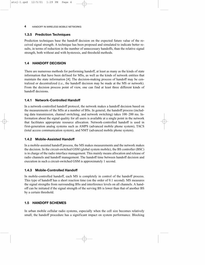
1.3.5 Prediction Techniques

Prediction techniques base the handoff decision on the expected future value of the re-ceived signal strength. A technique has been proposed and simulated to indicate better re-sults, in terms of reduction in the number of unnecessary handoffs, than the relative signalstrength, both without and with hysteresis, and threshold methods.

1.4 HANDOFF DECISION

There are numerous methods for performing handoff, at least as many as the kinds of stateinformation that have been defined for MSs, as well as the kinds of network entities thatmaintain the state information [4]. The decision-making process of handoff may be cen-tralized or decentralized (i.e., the handoff decision may be made at the MS or network).From the decision process point of view, one can find at least three different kinds ofhandoff decisions.

1.4.1 Network-Controlled Handoff

In a network-controlled handoff protocol, the network makes a handoff decision based onthe measurements of the MSs at a number of BSs. In general, the handoff process (includ-ing data transmission, channel switching, and network switching) takes 100–200 ms. In-formation about the signal quality for all users is available at a single point in the networkthat facilitates appropriate resource allocation. Network-controlled handoff is used infirst-generation analog systems such as AMPS (advanced mobile phone system), TACS(total access communication system), and NMT (advanced mobile phone system).

1.4.2 Mobile-Assisted Handoff

In a mobile-assisted handoff process, the MS makes measurements and the network makesthe decision. In the circuit-switched GSM (global system mobile), the BS controller (BSC)is in charge of the radio interface management. This mainly means allocation and release ofradio channels and handoff management. The handoff time between handoff decision andexecution in such a circuit-switched GSM is approximately 1 second.

1.4.3 Mobile-Controlled Handoff

In mobile-controlled handoff, each MS is completely in control of the handoff process.This type of handoff has a short reaction time (on the order of 0.1 second). MS measuresthe signal strengths from surrounding BSs and interference levels on all channels. A hand-off can be initiated if the signal strength of the serving BS is lower than that of another BSby a certain threshold.

1.5 HANDOFF SCHEMES

In urban mobile cellular radio systems, especially when the cell size becomes relativelysmall, the handoff procedure has a significant impact on system performance. Blocking


stoj-1.qxd 12/5/01 1:29 PM

probability of originating calls and the forced termination probability of ongoing calls arethe primary criteria for indicating performance. In this section, we describe several exist-ing traffic models and handoff schemes.

1.5.1 Traffic Model

For a mobile cellular radio system, it is important to establish a traffic model before ana-lyzing the performance of the system. Several traffic models have been established basedon different assumptions about user mobility. In the following subsection, we briefly intro-duce these traffic models.

1.5.1.1 Hong and Rappaport’s Traffic Model (Two-Dimensional) Hong and Rappaport propose a traffic model for a hexagonal cell (approximated by a cir-cle) [5]. They assume that the vehicles are spread evenly over the service area; thus, the lo-cation of a vehicle when a call is initiated by the user is uniformly distributed in the cell.They also assume that a vehicle initiating a call moves from the current location in any di-rection with equal probability and that this direction does not change while the vehicle re-mains in the cell.

From these assumptions they showed that the arrival rate of handoff calls is

�H = �O (1.1)

wherePh = the probability that a new call that is not blocked would require at least one hand-

offPhh = the probability that a call that has already been handed off successfully would re-

quire another handoffBO = the blocking probability of originating callsPf� = the probability of handoff failure�O = the arrival rate of originating calls in a cell

The probability density function (pdf) of channel holding time T in a cell is derived as

fT (t) = �Ce–�Ct + [ fTn(t) + �C fTh(t)] – [FTn(t) + �C FTh(t)] (1.2)

wherefTn(t) = the pdf of the random variable Tn as the dwell time in the cell for an originated

callfTh(t) = the pdf of the random variable Th as the dwell time in the cell for a handed-off

callFTn(t) = the cumulative distribution function (cdf) of the time Tn

FTh(t) = the cdf of the time Th

�Ce–�Ct

�1 + �C

e–�Ct

�1 + �C

Ph(1 – BO)��1 – Phh(1 – Pf�)

1.5 HANDOFF SCHEMES 5

stoj-1.qxd 12/5/01 1:29 PM

1/�C = the average call duration�C = Ph(1 – BO)/[1 – Phh(1 – Pf�)]

1.5.1.2 El-Dolil et al.’s Traffic Model (One-Dimensional) An extension of Hong and Rappaport’s traffic model to the case of highway microcellularradio network has been done by El-Dolil et al. [6]. The highway is segmented into micro-cells with small BSs radiating cigar-shaped mobile radio signals along the highway. Withthese assumptions, they showed that the arrival rate of handoff calls is

�H = (Rcj – Rsh)Phi + RshPhh (1.3)

wherePhi = the probability that a MS needs a handoff in cell iRcj = the average rate of total calls carried in cell jRsh = the rate of successful handoffs

The pdf of channel holding time T in a cell is derived as

fT (t) = � � e–(�C+�ni)t + � � e–(�C+�h)t (1.4)

where1/�ni = the average channel holding time in cell i for a originating call1/�h = the average channel holding time for a handoff call

G = the ratio of the offered rate of handoff requests to that of originating calls

1.5.1.3 Steele and Nofal’s Traffic Model (Two-Dimensional)Steele and Nofal [7] studied a traffic model based on city street microcells, catering topedestrians making calls while walking along a street. From their assumptions, theyshowed that the arrival rate of handoff calls is

�H = �6

m=1

[�O(1 – BO) Ph� + �h(1 – Pf�) Phh�] (1.5)

where� = the fraction of handoff calls to the current cell from the adjacent cells

�h = 3�O(1 – BO) PI�PI = the probability that a new call that is not blocked will require at least one handoff

The average channel holding time T in a cell is

T� = + + (1.6)�1(1 – �) + ��2��

�d + �C

�(1 + �2)��o + �C

(1 + �1)(1 – �)��

�w + �C

�C + �h�

1 + G

�C + �ni�

1 + G


stoj-1.qxd 12/5/01 1:29 PM

where1/�w = the average walking time of a pedestrian from the onset of the call until he

reaches the boundary of the cell1/�d = the average delay time a pedestrian spends waiting at the intersection to cross

the road1/�o = the average walking time of a pedestrian in the new cell

�1 = �wPdelay/(�d – �w)�2 = �oPdelay/(�d – �o)

Pdelay = PcrossPd, the proportion of pedestrians leaving the cell by crossing the road Pd = the probability that a pedestrian would be delayed when he crosses the road� = �H(1 – Pf�)/[�H(1 – Pf�) + �O(1 – BO)]

1.5.1.4 Xie and Kuek’s Traffic Model (One- and Two-Dimensional) This model assumes a uniform density of mobile users throughout an area and that a useris equally likely to move in any direction with respect to the cell border. From this as-sumption, Xie and Kuek [8] showed that the arrival rate of handoff calls is

�H = E[C] �c—dwell (1.7)

whereE[C] = the average number of calls in a cell

�c—dwell = the outgoing rate of mobile users.

The average channel holding time T in a cell is

T� = (1.8)

1.5.1.5 Zeng et al.’s Approximated Traffic Model (Any Dimensional) Zeng et al.’s model is based on Xie and Kuek’s traffic model [9]. Using Little’s formula,when the blocking probability of originating calls and the forced termination probabilityof handoff calls are small, the average numbers of occupied channels E[C] is approximat-ed by

E[C] � (1.9)

where 1/� is the average channel holding time in a cell.Therefore, the arrival rate of handoff calls is

�H � �O (1.10)

Xie and Kuek focused on the pdf of the speed of cell-crossing mobiles and refined pre-vious results by making use of biased sampling. The distribution of mobile speeds ofhandoff calls used in Hong and Rappaport’s traffic model has been adjusted by using

�c—dwell�

�C

�O + �H�

�

1��C + �c—dwell


stoj-1.qxd 12/5/01 1:29 PM

f *(v) = (1.11)

where f (v) is the pdf of the random variable V (speed of mobile users), and E[V] is the av-erage of the random variable V.

f *(v) leads to the conclusion that the probability of handoff in Hong and Rappaport’straffic model is a pessimistic one, because the speed distribution of handoff calls are notthe same as the overall speed distribution of all mobile users.

Steele’s traffic model is not adaptive for an irregular cell and vehicular users. In Zenget al.’s approximated traffic model, actual deviation from Xie and Kuek’s traffic model isrelatively small when the blocking probability of originating calls and the forced termina-tion probability of handoff calls are small.

1.5.2 Handoff Schemes in Single Traffic Systems

In this section, we introduce nonpriority, priority, and queuing handoff schemes for a sin-gle traffic system such as either a voice or a data system [6–14]. Before introducing theseschemes, we assume that a system has many cells, with each having S channels. The chan-nel holding time has an exponential distribution with mean rate �. Both originating andhandoff calls are generated in a cell according to Poisson processes, with mean rates �O

and �H, respectively. We assume the system with a homogeneous cell. We focus our atten-tion on a single cell (called the marked cell). Newly generated calls in the marked cell arelabeled originating calls (or new calls). A handoff request is generated in the marked cellwhen a channel holding MS approaches the marked cell from a neighboring cell with asignal strength below the handoff threshold.

1.5.2.1 Nonpriority SchemeIn this scheme, all S channels are shared by both originating and handoff request calls. TheBS handles a handoff request exactly in the same way as an originating call. Both kinds ofrequests are blocked if no free channel is available. The system model is shown in Figure1.3.

With the blocking call cleared (BCC) policy, we can describe the behavior of a cell as a(S + 1) states Markov process. Each state is labeled by an integer i (i = 0, 1, · · · , S), repre-

vf(v)�E[V]


S

.

.

2

1

Channels

�H

�

�O

Figure 1.3 A generic system model for handoff.

stoj-1.qxd 12/5/01 1:29 PM

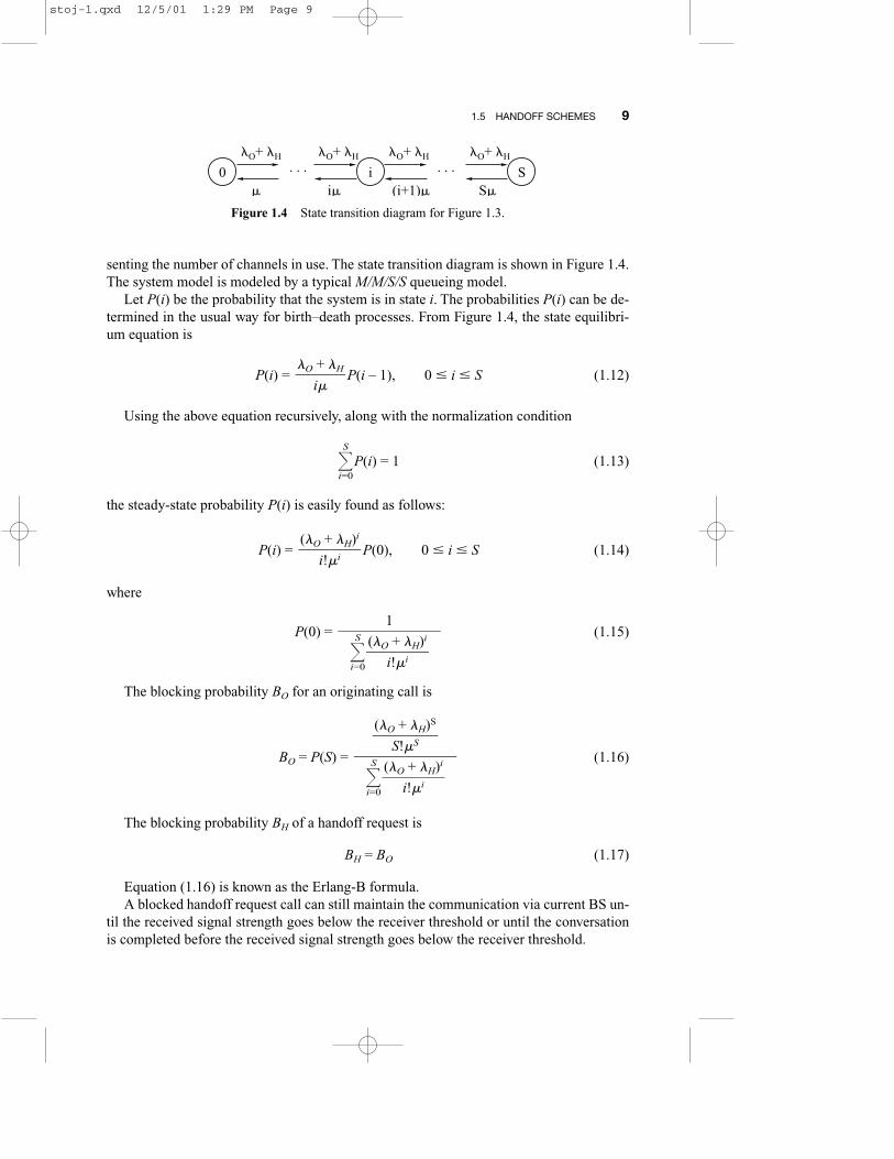
senting the number of channels in use. The state transition diagram is shown in Figure 1.4.The system model is modeled by a typical M/M/S/S queueing model.

Let P(i) be the probability that the system is in state i. The probabilities P(i) can be de-termined in the usual way for birth–death processes. From Figure 1.4, the state equilibri-um equation is

P(i) = P(i – 1), 0 � i � S (1.12)

Using the above equation recursively, along with the normalization condition

�S

i=0

P(i) = 1 (1.13)

the steady-state probability P(i) is easily found as follows:

P(i) = P(0), 0 � i � S (1.14)

where

P(0) = (1.15)

The blocking probability BO for an originating call is

BO = P(S) = (1.16)

The blocking probability BH of a handoff request is

BH = BO (1.17)

Equation (1.16) is known as the Erlang-B formula.A blocked handoff request call can still maintain the communication via current BS un-

til the received signal strength goes below the receiver threshold or until the conversationis completed before the received signal strength goes below the receiver threshold.

�(�O

S

+

!�

�S

H)S

�

��

�S

i=0

�(�O

i!

+

�

�i

H)i

�

1��

�S

i=0

�(�O

i!

+

�

�i

H)i

�

(�O + �H)i

��i!�i

�O + �H�

i�


Figure 1.4 State transition diagram for Figure 1.3.

0 · · ·

�O+ �H

�

i · · ·

�O+ �H

(i+1)�

�O+ �H

i�

S

�O+ �H

S�

stoj-1.qxd 12/5/01 1:29 PM

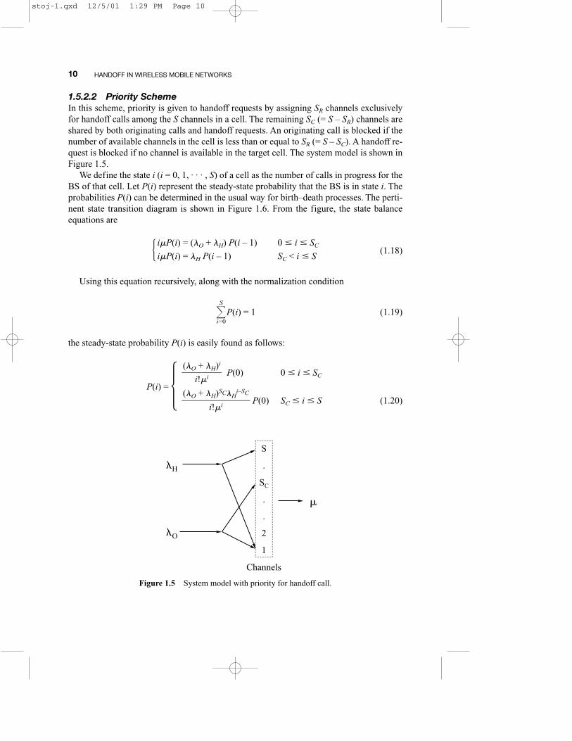
1.5.2.2 Priority SchemeIn this scheme, priority is given to handoff requests by assigning SR channels exclusivelyfor handoff calls among the S channels in a cell. The remaining SC (= S – SR) channels areshared by both originating calls and handoff requests. An originating call is blocked if thenumber of available channels in the cell is less than or equal to SR (= S – SC). A handoff re-quest is blocked if no channel is available in the target cell. The system model is shown inFigure 1.5.

We define the state i (i = 0, 1, · · · , S) of a cell as the number of calls in progress for theBS of that cell. Let P(i) represent the steady-state probability that the BS is in state i. Theprobabilities P(i) can be determined in the usual way for birth–death processes. The perti-nent state transition diagram is shown in Figure 1.6. From the figure, the state balanceequations are

� (1.18)

Using this equation recursively, along with the normalization condition

�S

i=0

P(i) = 1 (1.19)

the steady-state probability P(i) is easily found as follows:

�(�O

i!

+

�

�i

H)i

� P(0) 0 � i � SC

P(i) = � �(�O + �

iH

!�

)S

i

C�Hi–SC

� P(0) SC � i � S (1.20)

0 � i � SC

SC < i � S

i�P(i) = (�O + �H) P(i – 1)

i�P(i) = �H P(i – 1)


S

.

SC

.

.

2

1

Channels

�H

�O

�

Figure 1.5 System model with priority for handoff call.

stoj-1.qxd 12/5/01 1:29 PM

where

P(0) = ��SC

i=0

+ �S

i=SC+1�–1

(1.21)

The blocking probability BO for an originating call is given by

BO = �S

i=SC

P(i) (1.22)

The blocking probability BH of a handoff request is

BH = P(S) = P(0) (1.23)

Here again, a blocked handoff request call can still maintain the communication via cur-rent BS until the received signal strength goes below the receiver threshold or the conversa-tion is completed before the received signal strength goes below the receiver threshold.

1.5.2.3 Handoff Call Queuing SchemeThis scheme is based on the fact that adjacent cells in a mobile cellular radio system areoverlayed. Thus, there is a considerable area (i.e., handoff area) where a call can be han-dled by BSs in adjacent cells. The time a mobile user spent moving across the handoff areais referred as the degradation interval. In this scheme, we assume that the same channelsharing scheme is used as that of a priority scheme, except that queueing of handoff re-quests is allowed. The system model is shown in Figure 1.7.

To analyze this scheme, it is necessary to consider the handoff procedure in moredetail. When a MS moves away from the BS, the received signal strength decreases,and when it gets lower than a threshold level, the handoff procedure is initiated. Thehandoff area is defined as the area in which the average received signal strength of a MSreceiver from the BS is between the handoff threshold level and the receiver thresholdlevel.

If the BS finds all channels in the target cell occupied, a handoff request is put in thequeue. If a channel is released when the queue for handoff requests is not empty, thechannel is assigned to request on the top of the queue. If the received signal strengthfrom the current BS falls below the receiver threshold level prior to the mobile being as-signed a channel in the target cell, the call is forced to termination. The first-in-first-out

(�O + �H)SC�HS–SC

��S!�S

(�O + �H)SC�Hi–SC

��i!�i

(�O + �H)i

��i!�i



0 · · ·

�O+ �H

�

SC · · ·

�H

(SC+1)�

�O+ �H

SC�

S

�H

S�

stoj-1.qxd 12/5/01 1:29 PM

(FIFO) queueing strategy is used and infinite queue size at the BS is assumed. For a fi-nite queue size, see the discussion in the next secton. The duration of a MS in the hand-off area depends on system parameters such as the moving speed, the direction of theMS, and the cell size. We define this as the dwell time of a mobile in the handoff areaand denote it by random variable Th–dwell. For simplicity of analysis, we assume that thisdwell time is exponentially distributed with mean E[Th–dwell] (= 1/�h–dwell).

Let us define the state i (i = 0, 1, · · · , ) of a cell as the sum of channels being used inthe cell and the number of handoff requests in the queue. It is apparent from the above as-sumptions that i is a one-dimensional Markov chain. The state transition diagram of thecell is given in Figure 1.8. The equilibrium probabilities P(i) are related to each otherthrough the following state balance equations:

i�P(i) = (�O + �H)P(i – 1) 0 � i � SC

� i�P(i) = �HP(i – 1) SC < i � S (1.24)

[S� + (i – S)(�C + �h–dwell)] P(i) = �HP(i – 1) S < i �

Using the above equation recursively, along with the normalization condition of equa-tion (1.13), the steady-state probability P(i) is easily found as follows:

�(�O

i!

+

�

�i

H)i

�P(0) 0 � i � SC

P(i) = ��(�O + �

i!H

�

)S

i

C�Hi–SC

�P(0) SC < i � S (1.25)

�(�O

S

+

!�

�S

H)SC

� P(0) S < i � �H

i–SC

��i–S

�j=1

[S� + j(�C + �h–dwell)]


Figure 1.7 System model with priority and queue for handoff call.

S

.

SC

.

.

2

1

�H

Queue QH

Time-out Request

· · · 2 1

�O

�

stoj-1.qxd 12/5/01 1:29 PM

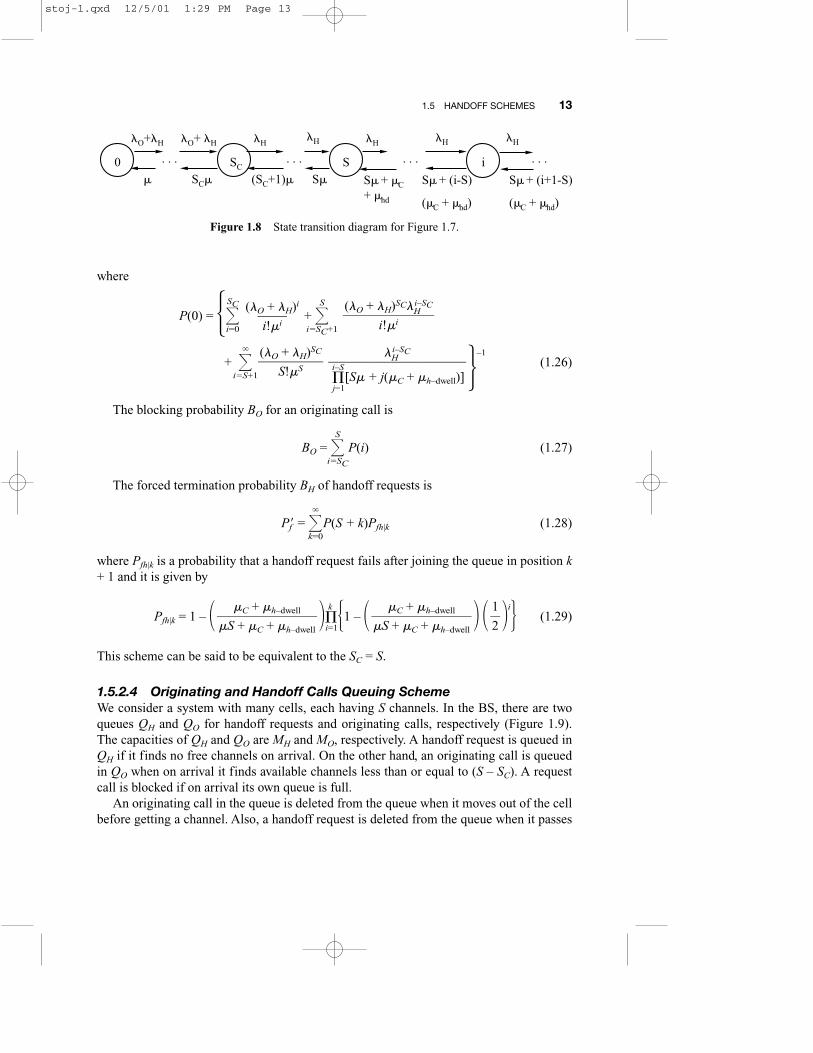
where

P(0) = ��SC

i=0

+ �S

i=SC+1

+ �

i=S+1

�(�O

S

+

!�

�S

H)SC

� –1

(1.26)

The blocking probability BO for an originating call is

BO = �S

i=SC

P(i) (1.27)

The forced termination probability BH of handoff requests is

Pf� = �

k=0

P(S + k)Pfh|k (1.28)

where Pfh|k is a probability that a handoff request fails after joining the queue in position k+ 1 and it is given by

Pfh|k = 1 – � � k

�i=1�1 – � � � �i (1.29)

This scheme can be said to be equivalent to the SC = S.

1.5.2.4 Originating and Handoff Calls Queuing Scheme We consider a system with many cells, each having S channels. In the BS, there are twoqueues QH and QO for handoff requests and originating calls, respectively (Figure 1.9).The capacities of QH and QO are MH and MO, respectively. A handoff request is queued inQH if it finds no free channels on arrival. On the other hand, an originating call is queuedin QO when on arrival it finds available channels less than or equal to (S – SC). A requestcall is blocked if on arrival its own queue is full.

An originating call in the queue is deleted from the queue when it moves out of the cellbefore getting a channel. Also, a handoff request is deleted from the queue when it passes

1�2

�C + �h–dwell��S + �C + �h–dwell

�C + �h–dwell��S + �C + �h–dwell

�Hi–SC

��i–S

�j=1

[S� + j(�C + �h–dwell)]

(�O + �H)SC�Hi–SC

��i!�i

(�O + �H)i

�i!�i


0 · · ·

�O+�H

�

SC · · ·

�H

(SC+1)�

�O+ �H

SC�

S

�H

S�

· · ·

�H

S�+ �C

+ �hd

i

�H

S�+ (i-S)

(�C + �hd)

�H

S�+ (i+1-S)

(�C + �hd)

· · ·


stoj-1.qxd 12/5/01 1:29 PM

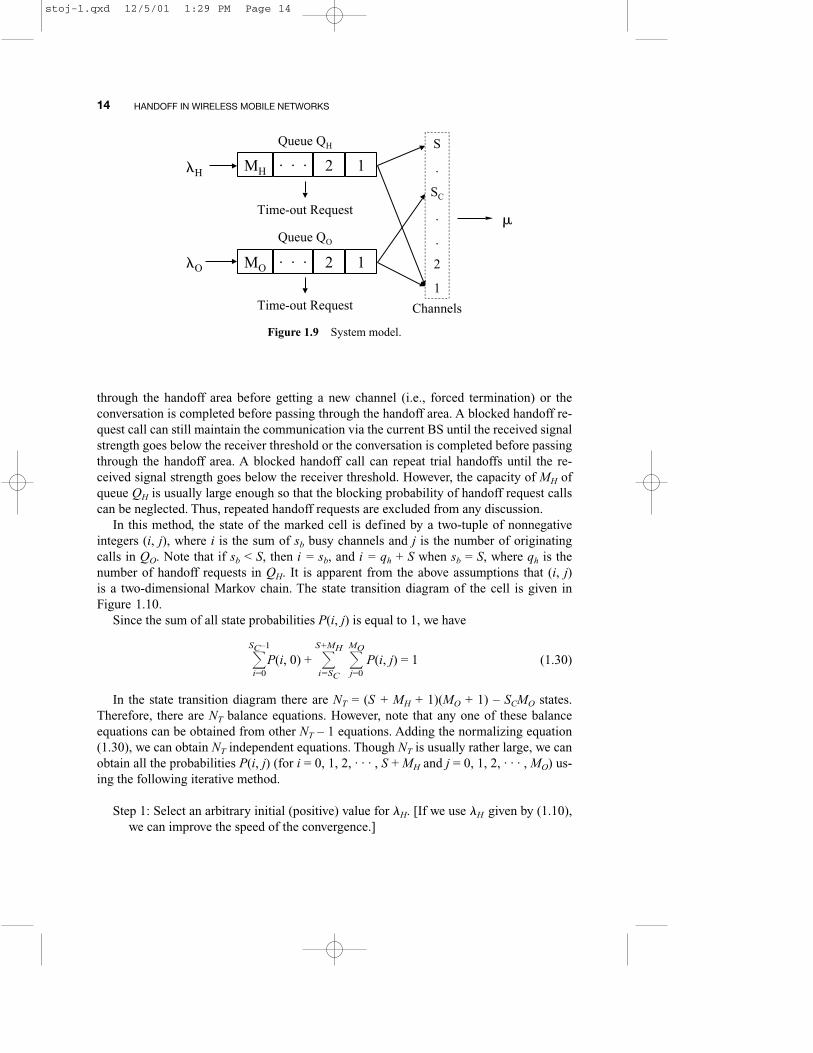
through the handoff area before getting a new channel (i.e., forced termination) or theconversation is completed before passing through the handoff area. A blocked handoff re-quest call can still maintain the communication via the current BS until the received signalstrength goes below the receiver threshold or the conversation is completed before passingthrough the handoff area. A blocked handoff call can repeat trial handoffs until the re-ceived signal strength goes below the receiver threshold. However, the capacity of MH ofqueue QH is usually large enough so that the blocking probability of handoff request callscan be neglected. Thus, repeated handoff requests are excluded from any discussion.

In this method, the state of the marked cell is defined by a two-tuple of nonnegativeintegers (i, j), where i is the sum of sb busy channels and j is the number of originatingcalls in QO. Note that if sb < S, then i = sb, and i = qh + S when sb = S, where qh is thenumber of handoff requests in QH. It is apparent from the above assumptions that (i, j)is a two-dimensional Markov chain. The state transition diagram of the cell is given inFigure 1.10.

Since the sum of all state probabilities P(i, j) is equal to 1, we have

�SC–1

i=0

P(i, 0) + �S+MH

i=SC

�MO

j=0

P(i, j) = 1 (1.30)

In the state transition diagram there are NT = (S + MH + 1)(MO + 1) – SCMO states.Therefore, there are NT balance equations. However, note that any one of these balanceequations can be obtained from other NT – 1 equations. Adding the normalizing equation(1.30), we can obtain NT independent equations. Though NT is usually rather large, we canobtain all the probabilities P(i, j) (for i = 0, 1, 2, · · · , S + MH and j = 0, 1, 2, · · · , MO) us-ing the following iterative method.

Step 1: Select an arbitrary initial (positive) value for �H. [If we use �H given by (1.10),we can improve the speed of the convergence.]


S

.

SC

.

.

2

1

Channels

�H

Queue QH

Time-out Request

MH · · · 2 1

�O

Queue QO

Time-out Request

MO · · · 2 1

�

Figure 1.9 System model.

stoj-1.qxd 12/5/01 1:29 PM

Step 2: Compute all the probabilities P(i, j) (for i = 0, 1, 2, · · · , S + MH and j = 0, 1,2, · · · , MO) using SOR (successive over-relation) method.

Step 3: Compute the average number of calls holding channels using the following for-mula:

E[C] = �SC–1

i=1

iP(i, 0) + �S

i=SC

i �MO

j=0

P(i, j) (1.31)

Step 4: Compute new �H substituting (1.31) into (1.7). If |new �H – old �H| � �, stopexecution. Otherwise, go to Step 2. Here � is a small positive number to check theconvergence.

Based on the above P(i, j)s, we can obtain the following performance measures of thesystem.

The blocking probability BO of an originating call is

BO = �S+MH

i=SC

P(i, MO) (1.32)

The blocking probability BH of a handoff request is equal to the probability of its ownqueue being filled up. Thus,

BH = �MO

j=0

P(S + MH, j) (1.33)


· · ·

�O+�

H

�

· · ·

�H

(SC+1)�

�O+ �

H

SC�

�H

S�

· · ·

�H

S�+ �c+

�h-dwell

�H

S�+ MH(�

c+

�h-dwell

)

S+MH, 0S, 0S

C, 00, 0

· · ·

�H

(SC+1)�

�H

S�

· · ·

�H

S�+ �c+

�h-dwell

�H

S�+MH(�

c

+ �h-dwell

)

S+MH, M

OS, MO

SC, M

O

···

S�+ �c-dwell

�O

S�+ MO

�c-dwell

�O

···

�c-dwell

�O

MO

�c-dwell

�O

···

�c-dwell

�O

MO.

�c-dwell

�O

Figure 1.10 State transition diagram.

stoj-1.qxd 12/5/01 1:29 PM

The average LO length of queue QO is:

LO = �MO

j=1

j �S+MH

i=SC

P(i, j) (1.34)

and the average length LN of queue QH is:

LH = �S+MH

i=S+1

(i – S) �MO

j=0

P(i, j) (1.35)

Since the average number of originating calls arrived and deleted from the queue inunit time are (1 – BO)�O and �c—dwellLO, respectively, the time-out probability of originat-ing calls is given by

PO–out = (1.36)

Similarly, the time-out probability of handoff request calls in the queue QH is given by

PH–out = (1.37)

Therefore, the probability of an originating call not being assigned a channel and theforced termination probability of a handoff request are given by

PO = BO + (1 – BO)FO–out (1.38)

and

Pf� = BH + (1 – BH)PH–out (1.39)

Once a MS is assigned to a channel and if a call is in progress, any subsequent cellboundary crossings necessitates further handoffs. The handoff probability Ph of a call isthe probability that the call holding time TC (random variable) exceeds the dwell timeTc—dwell (random variable) of the user in a cell, i.e.,

Ph = Pr{TC > Tc—dwell} (1.40)

Assuming that TC and Tc—dwell are independent, we can easily get

Ph = (1.41)

The forced termination probability Pf that a call accepted by the system is forced toterminate during its lifetime is a true measure of the system performance. It is important

�c—dwell��C + �c—dwell

�h–dwellLH��(1 – BH)�H

�c—dwellLO��(1 – BO)�O


stoj-1.qxd 12/5/01 1:29 PM

to distinguish between this probability and the failure probability Pf� of a single handoffattempt. The forced termination probability Pf of handoff calls can be expressed as

Pf = �

l=1

PhPf�[(1 – Pf�) Ph]l–1 = (1.42)

For special situations, solutions are already known for the case of MH = and MH = 0when MO = 0. In the system with MH = finite, an originating call is blocked if the numberof available channels in the cell is less than or equal to S – SC. A handoff request isblocked if on arrival it finds that QH is filled.

In this case, we consider the case for MO = 0. The two-dimensional state-transition dia-gram becomes one-dimensional ( j = 0). Therefore, the state probabilities can easily be ob-tained as follows:

�a

i!

i

�P(0, 0) 0 � i � SC

��a

b��SC

�b

i!

i

�P(0, 0) SC � i � SP(i,0) = � (1.43)

S + 1 � i � S + MH

where a = , b = , and h = ,

P(0,0) = ��SC

i=0

+ ��a

b��SC �

S

i=SC+1

+ �S+MH

i=S+1 –1

(1.44)

and

�H = E[C] �c—dwell = �c—dwell �S

i=1

iP(i, 0) (1.45)

Therefore, the blocking probability BO of an originating call is

BO = �S+MH

i=SC

P(i, 0)

= � + ��a

b��SC �

S

i=SC+1

+ �S+MH

i=S+1 � P(0, 0). (1.46)bi

��i–S

�j=1

(S + jh)

��a

b��SC

�S!

bi

�i!

aSC

�SC!

bi

��i–S

�j=1

(S + jh)

��a

b��SC

�S!

bi

�i!

ai

�i!

�C + �h–dwell��

�

�H��

�O + �H�

�

biP(0, 0)��i–S

�j=1

(S + jh)

��a

b��SC

�S!

PhPf��1 – Ph(1 – Pf�)


stoj-1.qxd 12/5/01 1:29 PM

The average length LH of queue QH is

LH = �S+MH

i=S+1

(i – S)P(i, 0). (1.47)

1.5.3 Handoff Schemes in Multiple Traffic Systems

In this section, we discuss nonpreemptive and preemptive priority handoff schemes for amultiple traffic system, such as an integrated voice and data system or integrated real-timeand nonreal-time system. Although we focus our attention just on integrated voice anddata systems, the results can be extended to other similar systems. Before introducingthese schemes, we make the following assumptions for our discussion. The call holdingtime TCV of voice calls is assumed to have an exponential distribution with mean E[TCV](= 1/�CV). The data length TCD is also assumed to have an exponential distribution withmean E[TCD] (= 1/�CD). The dwell time Tc–dwell (the random variable) of mobile users in acell is assumed to have an exponential distribution with mean E[Tc—dwell] (= 1/�c—dwell).The random variable Th–dwell is defined as the time spent in the handoff area by voicehandoff request calls and is assumed to have an exponential distribution with meanE[Tc—dwell] (= 1/�c—dwell). The channel holding time of a voice (or data) call is equal to thesmaller one between Tc–dwell and TCV (or TCD). Using the memoryless property of the ex-ponential pdf, we see that the random variables TV and TD (the channel holding time ofvoice and data calls) are both exponentially distributed, with means E[TV] [= 1/�V =1/(�CV + �c—dwell)] and E[TD] [= 1/�D = 1/(�CD + �c—dwell)], respectively. We assume thatthe arrival processes of originating voice and data calls and voice and data handoff calls ina cell are Poisson. The arrival rates of originating voice and data calls are designated as�OV and �OD, respectively. We denote the arrival rates of voice and data handoff requestsby �HV and �HD, respectively. A data handoff request in the queue of the current cell istransferred to the queue of target cell when it moves out of the cell before getting a chan-nel. The transfer rate is given by

�time—out = Lqd�c—dwell (1.48)

where Lqd is the average length of data queue.We define a new variable �HT by

�HT = �HD + �time—out = ND�c—dwell (1.49)

where ND is the average number of data handoff requests in a cell.

1.5.3.1 Nonpreemptive Priority Handoff SchemeWe consider a system with many cells each having S channels. As the system is assumedto have homogeneous cells, we focus our attention on a single cell called the marked cell.A system model is shown in Figure 1.11. In each BS, there are two queues, QV and QD,with capacities MV and MD for voice and data handoff requests, respectively.

Newly generated calls in the marked cell are called originating calls. For voice users,there is a handoff area. For data users, the boundary is defined as the locus of points where


stoj-1.qxd 12/5/01 1:29 PM

the average received signal strength of the two neighboring cells are equal. The process ofgeneration for handoff request is same as in previous schemes.

A voice handoff request is queued in QV on arrival if it finds no idle channels. On theother hand, a data handoff request is queued in QD on arrival when it finds (S – Sd) or few-er available channels, where Sd is the number of usable channels for data handoff users.An originating voice or an originating data call is blocked on arrival if it finds (S – Sc) orfewer available channels, where Sc is the number of channels for both originating calls. Noqueue is assumed here for originating calls. A handoff request is blocked if its own queueis full on its arrival.

If there are channels available, the voice handoff request calls in QV are served basedon the FIFO rule. If more than (S – Sd) channels are free, the data handoff request calls inQD are served by the FIFO rule. A voice handoff request in the queue is deleted from thequeue when it passes through the handoff area before getting a new channel (i.e., forcedtermination) or its communication is completed before passing through the handoff area.A data handoff request can be transferred from the queue of the current cell to the one ofthe target cells when it moves out of the current cell before getting a channel.

A blocked voice handoff request maintains communication via the current BS until thereceived signal strength falls below the receiver threshold or the conversation is completedbefore passing through the handoff area. However, the probability of a blocked voicehandoff request call completing the communication before passing through the handoffarea is neglected. A blocked voice handoff request can repeat trial handoffs until the re-ceived signal strength goes below the receiver threshold. However, the capacities of MV

and MD of queues are usually large enough so that the blocking probability of handoff re-quest calls can be neglected. Thus, repeated trials of blocked handoff requests are exclud-ed from any discussion.

The state of the marked cell is defined by a three-tuple of nonnegative integers (i, j, k),


S

.

Sd

.

Sc

.

2

1

Queue QD

Originating Voice and Data Calls

Total Data Handoff Request

Voice Handoff Request

Channels

Data Handoff

Call Completed

Voice Handoff

Time-out Request

�HV

�HD

�O

�T

�HV

�HD

�HT

Queue QV

Time-out Request S

.

Sd

.

Sc

.

2

1

Queue QD

Originating Voice and Data Calls

Total Data Handoff Request

Voice Handoff Request

Channels

Data Handoff

Call Completed

Voice Handoff

Time-out Request

�HV

�HD

�O

�T

�HV

�HD

�HT

Queue QV

Time-out Request

Figure 1.11 System model with two queues for handoffs.

stoj-1.qxd 12/5/01 1:29 PM

where i is the sum of the number of channels used by voice calls (including originatingcalls and handoff requests) and the number of voice handoff requests in the queue QV, j isthe number of channels used by data handoff requests, and k is the number of data handoffrequests in the queue QD. It is apparent from the above assumptions that (i, j, k) is a three-dimensional Markov chain.

In the state transition diagram, there are NT = (S + MV – Sd + 1)(Sd + 1)(MD + 1) + Sd(Sd

+ 1)/2 states. Therefore, the state transition diagram leads to NT balance equations. Equi-librium probabilities P(i, j, k) are related to each other through the state balance equations.However, note that any one of these balance equations can be obtained from other NT – 1equations. Since the sum of all state probabilities is equal to 1, we have

�Sd

j=0�

S+MV–j

i=0

P(i, j, 0) + �Sd

j=0�

S+MV–j

i=Sd–j�MD

k=1

P(i, j, k) = 1 (1.50)

Adding the normalizing equation (1.50), we can obtain NT independent equations inwhich �HV and �HT are two unknown variables. Using equation (1.7), we can get

�HV = E[CV] �c—dwell (1.51)

Adding equations (1.49) and (1.51) leads to NT + 2 nonlinear independent simultaneousequations. Though NT is usually rather large, all the probabilities P(j, j, k) (for i = 0, 1, 2, .. . , S + MV; j = 0, 1, 2, . . . , Sd, and k = 0, 1, 2, . . . , MD) can be obtained by solving NT + 2nonlinear independent simultaneous equations, as illustrated in the next section.

Step 1: Select arbitrary initial (positive) values for �HV and �HT.

Step 2: Compute all the probabilities P(i, j, k) (for i = 0, 1, 2, . . . , S + MV, j = 0, 1,2, . . . , Sd, and k = 0, 1, 2, . . . , MD) using the SOR method.

Step 3: Compute the average numbers E[CV] of voice calls holding channels, and com-pute the average numbers ND of data channel requests in a cell using the followingrelations:

E[CV] = �S–Sd

i=0

i �Sd

j=0�MD

k=0

P(i, j, k) + �S

i=S–Sd+1

i �S–i

j=0�MD

k=0

P(i, j, k)

+ �Sd

j=0

(S – j) �S+MV–j

i=S–j+1�MD

k=0

P(i, j, k) (1.52)

and

ND = �Sd

j=1

j �S+MV–j

i=0�MD

k=0

P(i, j, k) + �MD

k=1

k �Sd

j=0�

S+MV–j

i=Sd–j

P(i, j, k) (1.53)

Step 4: Compute new �HV by substituting (1.52) into (1.51). Compute new �HT by sub-stituting (1.53) into (1.49). If |new �HV – old �HV| � � and |new �HT – old �HT| � �,


stoj-1.qxd 12/5/01 1:29 PM

stop execution. Otherwise, go to Step 2. Here � is a small positive number to checkthe convergence.

Based on the above P(i, j, k)s, we can obtain the following performance measures ofthe system.

The blocking probability of an originating voice call or originating data call is

BO = BOV = BOD = �Sd

j=0�

S+MV–j

i=SV–j �MD

k=0

P(i, j, k) (1.54)

The blocking probability BHV of a voice handoff request is

BHV = �Sd

j=0�MD

k=0

P(S + MV – j, j, k) (1.55)

The blocking probability BHD of a data handoff request is

BHD = �Sd

j=0�

S+MV–j

i=Sd–j

P(i, j, MD) (1.56)

The average length Lqv of queue QV is

Lqv = �S+MV

i=S+1

(i – S)�Sd

j=0�MD

k=0

P(i – j, j, k) (1.57)

The average length Lqd of queue QD is

Lqd = �MD

k=1

k �Sd

j=0�

S+MV–j

i=Sd–j

P(i, j, k) (1.58)

Since the average number of voice handoff requests arrived and deleted in unit time are(1 – BHV)�HV and �h–dwellLqv, respectively, the time-out probability of a voice handoff re-quests in the queue QV is given by

PV–out = (1.59)

Therefore, failure probability of a voice handoff request for single handoff attempt is

P�fV = BHV + (1 – BHV) PV–out (1.60)

The voice user in a cell is given by

Ph = Pr{TCV > Tc–dwell} (1.61)

�h–dwellLqv��(1 – BHV)�HV


stoj-1.qxd 12/5/01 1:29 PM

Assuming that TCV and Tc–dwell are independent, we can easily get

Ph = (1.62)

The forced termination probability PfV of voice calls can be expressed as

PfV = �

l=1

PhP�fV[(1 – P�fV) Ph]l–1 = (1.63)

Using Little’s formula, the average value of waiting time TW of data handoff requests inthe queue is given by

TW = (1.64)

Average value of time TS (random variable) of a call in a cell is

TS = (1.65)

Let us define Nh as the average number of handoffs per data handoff request during itslifetime. Thus, we have

Nh = �NhTW +

TS

E[TCD]� (1.66)

Then,

Nh = (1.67)

where

E[CD] = �Sd

j=1

j �S+MV–j

i=0�MD

k=0

P(i, j, k) (1.68)

Therefore, the average transmission delay (except average data length) Tdelay of data is

Tdelay = NhTW = (1.69)Lqd

��E[CD] �CD

(1 – BOD) �OD + (1 – BHD) �HT��

E[CD] �CD

ND��(1 – BOD) �OD + (1 – BHD) �HT

Lqd��(1 – BOD) �OD + (1 – BHD) �HT

PhP�fV��1 – Ph(1 – P�fV)

�c—dwell��CV + �c—dwell


stoj-1.qxd 12/5/01 1:29 PM

1.5.3.2 Preemptive Priority Handoff SchemeThis scheme is a modification of a nonpreemptive priority handoff scheme, with higherpriorities for voice handoff request calls. In this scheme, a handoff request call is served ifthere are channels available when such a voice handoff request call arrives. Otherwise, thevoice handoff request can preempt the data call, when we assume there is an ongoing datacall, if on arrival it finds no idle channel. The interrupted data call is returned to the dataqueue QD and waits for a channel to be available based on the FIFO rule. A voice handoffrequest is queued in QV by the system if all the channels are occupied by prior calls andthe data queue QD is full (i.e., data calls cannot be preempted by voice handoff calls whenthe data queue QD is full). It is possible to think of another scheme where data calls in ser-vice can be preempted by voice handoff calls irrespective of whether the queue QD is fullor not. However, the same effect can be observed if the queue capacity is increased to arelatively large value.

The same state of the marked cell is assumed and represented by a three-tuple of non-negative integers (i, j, k) as defined in the nonpreemptive priority handoff scheme. In thestate transition diagram for the three-dimensional Markov chain model there are NT = (S –Sd + 1)(Sd + 1)(MD + 1) + (Sd + MD + 1)MV + Sd(Sd + 1)/2 states. Therefore, as in the non-preemptive priority handoff scheme, we can get NT balance equations through the state tran-sition diagram. Equilibrium probabilities P(i, j, k) are related to each other through the statebalance equations. However, note that any one of these balance equations can be obtainedfrom other NT – 1 equations. Since the sum of all state probabilities is equal to 1, we have

�Sd

j=0�S–j

i=0

P(i, j, 0) + �Sd

j=0�S–j

i=Sd–j�MD

k=1

P(i, j, k) + �S+MV

i=S+1 �MD

k=0

P(i, 0, k)

+ �Sd

j=1�

S+MV–j

i=S–j+1

P(i, j, MD) = 1 (1.70)

The probabilities P(j, j, k) (for i = 0, 1, 2, . . . , S + MV ; j = 0, 1, 2, . . . , Sd, and k = 0, 1,2, . . . , MD) can be obtained by using the same method of computation in the nonpreemp-tive priority handoff scheme. The differences are:

E[CV] = �S–Sd

i=0

i �Sd

j=0�MD

k=0

P(i, j, k) + �S

i=S–Sd+1

i �S–i

j=0�MD

k=0

P(i, j, k)\

+ �Sd

j=0

(S – j) �S+MV–j

i=S–j+1

P(i, j, MD) (1.71)

ND = �Sd

j=1

j �S–j

i=0�MD

k=0

P(i, j, k) + �Sd

j=1

j �S+MV–j

i=S–j+1

P(i, j, MD) + �MD

k=1

k �Sd

j=0�S–j

i=Sd–j

P(i, j, k)

+ �MD–1

k=1

k �S+MV

i=S+1

P(i, 0, k) + MD �Sd

j=0�

S+MV–j

i=S–j+1

P(i, j, MD) (1.72)


stoj-1.qxd 12/5/01 1:29 PM

and

E[CD] = �Sd

j=1

j �S–j

i=0�MD

k=0

P(i, j, k) + �Sd

j=1

j �S+MV–j

i=S–j+1

P(i, j, MD) (1.73)

Therefore, the performance measurements can be obtained by equations (1.54)–(1.69).

1.6 SUMMARY

The basic concept of handoff in mobile cellular radio systems has been introduced. Sever-al different traffic models have been described and briefly discussed. Four conventionalhandoff schemes in single traffic systems—i.e., nonpriority scheme, priority scheme,handoff call queueing scheme, and originating and handoff call queuing schemes—havebeen summarized in this chapter. The two handoff schemes with and without preemptivepriority procedures for integrated voice and data wireless mobile networks have also beencovered in detail.

REFERENCES

1. M. Gudmundson, Analysis of handover algorithms, Proc. IEEE VTC ’91, pp. 537–542, May1991.

2. V. Kapoor, G. Edwards, and R. Snkar, Handoff criteria for personal communication networks,Proc. IEEE ICC ’94, pp. 1297–1301, May 1994.

3. G. P. Pollini, Trends in handover design, IEEE Commun. Magazine, pp. 82–90, March 1996.

4. N. D. Tripathi, J. H. Reed, and H. F. Vanlandingham, Handoff in Cellular Systems, IEEE Per-sonal Commun., December 1998.

5. D. Hong and S. S. Rappaport, Traffic model and performance analysis for cellular mobile radiotelephone systems with prioritized and nonprioritized handoff procedures, IEEE Trans. Veh.Technol., Vol. VT-35, No. 3, pp. 448–461, August 1986.

6. S. A. El-Dolil, W. C. Wong, and R. Steele, Teletraffic performance of highway microcells withoverlay macrocell, IEEE J. Select. Areas in Commun., Vol. 7, No. 1, pp. 71–78, January 1989.

7. R. Steele and M. Nofal, Teletraffic performance of microcellular personal communication net-works, IEE PROCEEDINGS-I, Vol. 139, No. 4, August 1992.

8. H. Xie and S. Kuek Priority handoff analysis, Proc. IEEE VTC ’93, pp. 855–858, 1993.

9. Q-A. Zeng, K. Mukumoto, and A. Fukuda, Performance analysis of mobile cellular radio sys-tems with two-level priority reservation handoff procedure, IEICE Trans. Commun., Vol. E80-B,No. 4, pp. 598–604, April 1997.

10. S. Tekinay and B. Jabbari, A measurement-based prioritization scheme for handovers in mobilecellular networks, IEEE J. Select. Areas in Commun., Vol. 10, No. 8, Oct. 1992.

11. Q-A. Zeng, K. Mukumoto, and A. Fukuda, Performance analysis of mobile cellular radio sys-tems with priority reservation handoff procedures, Proc. IEEE VTC ’94, Vol. 3, pp. 1829–1833,June 1994.


stoj-1.qxd 12/5/01 1:29 PM

12. R. B. Cooper, Introduction to Queueing Theory, 2nd ed. New York: Elsevier North Holland,1981.

13. J. D. Wells, Cellular system design using the expansion cell layout method, IEEE Trans. Veh.Technol., Vol. VT-33, May 1984.

14. H. Akimaru and R. B. Cooper, Teletraffic Engineering. Ohm, 1985.

15. Q-A. Zeng and D. P. Agrawal, Performance analysis of a handoff scheme in integratedvoice/data wireless networks, Proc. IEEE VTC 2000 Fall, Vol. 4, pp. 1986–1992, September2000.

16. Q-A. Zeng and D. P. Agrawal, An analytical modeling of handoff for integrated voice/data wire-less networks with priority reservation and preemptive priority procedures, Proc. ICPP 2000Workshop on Wireless Networks and Mobile Computing, pp. 523–529, August 2000.

REFERENCES 25

stoj-1.qxd 12/5/01 1:29 PM

stoj-1.qxd 12/5/01 1:29 PM

chapter 1 handoff in wireless mobile networks · handoff in wireless mobile networks ... (or...

Documents