chapter 1. addendum overview: centrality, pinch-point, and

Columbia Plateau Ecoregion Addendum: Habitat Connectivity Centrality, Pinch-Points, and Barriers/Restoration Analyses 1.1

Chapter 1. Addendum Overview: Centrality, Pinch-Point, and Barrier and Restoration Analyses

Prepared by Joanne Schuett-Hames (WDFW), Leslie Robb (Independent Researcher), and Brad McRae

(TNC)

This addendum to the Washington Connected Landscapes

Project: Analysis of the Columbia Plateau Ecoregion

(WHCWG 2012; Available from http://waconnected.org),

presents supplemental connectivity mapping products for

the Columbia Plateau Ecoregion. These supplemental maps

were produced using new spatial analysis tools (McRae

2012a, 2012b, 2012c; McRae et al. 2012) developed to help

inform, prioritize, and implement connectivity conservation

action.

The analyses presented in the addendum build upon the

landscape resistance surfaces, cost-weighted distance

surfaces, and linkage networks modeled for eleven focal

species in the Columbia Plateau Ecoregion and a

surrounding buffer area (WHCWG 2012). We include

supplemental connectivity maps for each of the focal species (See Chapters 2–12), as well as composite

maps that summarize important patterns across all focal species (See Chapter 13).

The supplemental products include maps, interpretive examples, and GIS files depicting: (1) linkage

network centrality, (2) linkage pinch-points, and (3) barriers and restoration opportunities. We

emphasize that we do not provide a full interpretation or prioritization of the connectivity products, and our

results have not been verified by field studies. We do provide guidance for interpretation of these products

for the Columbia Plateau and present examples of potential applications for conservation.

In this chapter we describe the connectivity products provided in this document and include example figures

to acquaint readers with information found in Chapters 2–13. Additional background information is

presented in the sidebar text of the full-scale centrality, pinch-point, and barrier/restoration opportunities

maps presented in Chapters 2–13. Each chapter additionally includes interpretive figures that highlight and

explain example areas of interest. GIS files are available from http://waconnected.org.

Questions and Decisions these Analyses Help Inform

Where are important areas on the landscape for maintaining connectedness?

Where should further disturbance to connectivity be avoided?

Where along linkages is potential movement highly or moderately constrained?

Are there areas where alternative movement routes may not be available?

Where in a linkage will restoration efforts have the greatest effect on connectivity?

Where can alternate linkage pathways be created by restoration of key areas or removal of barriers?

Which habitat concentration areas (HCAs) might be important for species recovery efforts (e.g., sites

for translocations and augmentations of populations)?

Where would it be useful to collect genetic or other data on population connectivity?

What areas act as important HCAs, corridors, pinch-points, or barriers for multiple species?

Linkage Network Centrality (See example Figures 1.1–1.3)

Centrality is a measure of how important a habitat area or linkage is for maintaining movement among all or

many locations across a landscape (Estrada & Bodin 2008; Carroll et al. 2012). Our analyses start with

linkage networks modeled for the Columbia Plateau Ecoregion (WHCWG 2012), and seek to identify which

habitat concentration areas (HCAs) and linkages are most important for keeping those networks connected.

Linkages or HCAs with high centrality are important for maintaining movement between many HCAs, and

can be thought of as ―gatekeepers‖ for connectivity. For example, if a linkage with high centrality is

severed, a wildlife species may risk having its population separated into sub-populations.

Linkage Pinch-Points (See example Figures 1.4–1.7)

Pinch-points (also known as bottlenecks or choke-points) are areas where animal movement is funneled

within linkages. Pinch-point modeling methods are based on current flow models from electrical circuit

theory. Locations where current is very strong indicates constrictions where linkages are most vulnerable to

being severed (McRae et al. 2008).

Pinch-points can be the result of both natural and human-made landscape features. Pinch-points may be

conservation priorities as they are locations where loss of a small area could disproportionately compromise

connectivity because alternative movement routes are unavailable. Loss of these areas may sever migration

routes or impact other important movement needs. To determine the relative importance of pinch-points in

different linkages, users should consider pinch-point results along with other measures such as centrality.

Barriers and Restoration Opportunities (See example Figures 1.8–1.11)

Barriers are areas where landscape features impede wildlife movement between HCAs. Barriers may be

partial or complete, natural (e.g., rivers, cliffs) or human-made (e.g., urban areas, highways, some types of

agriculture), and some but not all barriers may be restorable.

Barrier mapping complements corridor mapping by broadening the range of connectivity conservation

alternatives available to practitioners. It can help identify areas where connectivity can be restored through

active barrier removal. It can inform decisions on trade-offs between restoration and protection; for

example, purchasing an intact corridor may be substantially more expensive than restoring a barrier that

blocks an alternative corridor. Barrier maps can also help identify corridors that are too degraded to provide

meaningful movement opportunities (McRae et al. 2012).

Composite Map Products (See example Figure 1.12)

In Chapter 13, we present composite maps that integrate the results for centrality, pinch-point, and barriers

and restoration opportunities analyses across all focal species. These maps help to show where conservation

Dry Falls, photo by Joe Rocchio

http://waconnected.org/

http://waconnected.org/


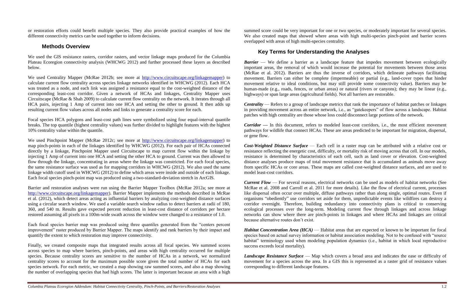
or restoration efforts could benefit multiple species. They also provide practical examples of how the

different connectivity metrics can be used together to inform decisions.

Methods Overview

We used the GIS resistance rasters, corridor rasters, and vector linkage maps produced for the Columbia

Plateau Ecoregion connectivity analysis (WHCWG 2012) and further processed these layers as described

below.

We used Centrality Mapper (McRae 2012b; see more at http://www.circuitscape.org/linkagemapper) to

calculate current flow centrality across species linkage networks identified in WHCWG (2012). Each HCA

was treated as a node, and each link was assigned a resistance equal to the cost-weighted distance of the

corresponding least-cost corridor. Given a network of HCAs and linkages, Centrality Mapper uses

Circuitscape (McRae & Shah 2009) to calculate current flow centrality on the network. It iterates through all

HCA pairs, injecting 1 Amp of current into one HCA and setting the other to ground. It then adds up

resulting current flow values across all nodes and links to generate a centrality score for each.

Focal species HCA polygons and least-cost path lines were symbolized using four equal-interval quantile

breaks. The top quantile (highest centrality values) was further divided to highlight features with the highest

10% centrality value within the quantile.

We used Pinchpoint Mapper (McRae 2012c; see more at http://www.circuitscape.org/linkagemapper) to

map pinch-points in each of the linkages identified by WHCWG (2012). For each pair of HCAs connected

directly by a linkage, Pinchpoint Mapper used Circuitscape to map current flow within the linkage by

injecting 1 Amp of current into one HCA and setting the other HCA to ground. Current was then allowed to

flow through the linkage, concentrating in areas where the linkage was constricted. For each focal species,

the same resistance surface was used as for mapping corridors in WHCWG (2012). We also used the same

linkage width cutoff used in WHCWG (2012) to define which areas were inside and outside of each linkage.

Each focal species pinch-point map was produced using a two-standard-deviation stretch in ArcGIS.

Barrier and restoration analyses were run using the Barrier Mapper Toolbox (McRae 2012a; see more at

http://www.circuitscape.org/linkagemapper). Barrier Mapper implements the methods described in McRae

et al. (2012), which detect areas acting as influential barriers by analyzing cost-weighted distance surfaces

using a circular search window. We used a variable search window radius to detect barriers at radii of 180,

360, and 540 m. Results gave expected percent reduction in least-cost distance of corridors per hectare

restored assuming all pixels in a 100m-wide swath across the window were changed to a resistance of 1.0.

Each focal species barrier map was produced using three quantiles generated from the ―centers percent

improvement‖ raster produced by Barrier Mapper. The maps identify and rank barriers by their impact and

quantify the extent to which restoration may improve connectivity.

Finally, we created composite maps that integrated results across all focal species. We summed scores

across species to map where barriers, pinch-points, and areas with high centrality occurred for multiple

species. Because centrality scores are sensitive to the number of HCAs in a network, we normalized

centrality scores to account for the maximum possible score given the total number of HCAs for each

species network. For each metric, we created a map showing raw summed scores, and also a map showing

the number of overlapping species that had high scores. The latter is important because an area with a high

summed score could be very important for one or two species, or moderately important for several species.

We also created maps that showed where areas with high multi-species pinch-point and barrier scores

overlapped with areas of high multi-species centrality.

Key Terms for Understanding the Analyses

Barrier — We define a barrier as a landscape feature that impedes movement between ecologically

important areas, the removal of which would increase the potential for movements between those areas

(McRae et al. 2012). Barriers are thus the inverse of corridors, which delineate pathways facilitating

movement. Barriers can either be complete (impermeable) or partial (e.g., land-cover types that hinder

movement relative to ideal conditions, but may still provide some connectivity value). Barriers may be

human-made (e.g., roads, fences, or urban areas) or natural (rivers or canyons); they may be linear (e.g.,

highways) or span large areas (agricultural fields). Not all barriers are restorable.

Centrality — Refers to a group of landscape metrics that rank the importance of habitat patches or linkages

in providing movement across an entire network, i.e., as ―gatekeepers‖ of flow across a landscape. Habitat

patches with high centrality are those whose loss could disconnect large portions of the network.

Corridor — In this document, refers to modeled least-cost corridors, i.e., the most efficient movement

pathways for wildlife that connect HCAs. These are areas predicted to be important for migration, dispersal,

or gene flow.

Cost-Weighted Distance Surface — Each cell in a raster map can be attributed with a relative cost or

resistance reflecting the energetic cost, difficulty, or mortality risk of moving across that cell. In our models,

resistance is determined by characteristics of each cell, such as land cover or elevation. Cost-weighted

distance analyses produce maps of total movement resistance that is accumulated as animals move away

from specific HCAs or core areas. These maps are called cost-weighted distance surfaces, and are used to

model least-cost corridors.

Current Flow — For several reasons, electrical networks can be used as models of habitat networks (See

McRae et al. 2008 and Carroll et al. 2011 for more details). Like the flow of electrical current, processes

like dispersal often occur over multiple, diffuse pathways rather than along single, optimal routes. Even if

organisms ―obediently‖ use corridors set aside for them, unpredictable events like wildfires can destroy a

corridor overnight. Therefore, building redundancy into connectivity plans is critical to conserving

ecological processes over the long-term. Modeling current flow through linkages and across linkage

networks can show where there are pinch-points in linkages and where HCAs and linkages are critical

because alternative routes don’t exist.

Habitat Concentration Area (HCA) — Habitat areas that are expected or known to be important for focal

species based on actual survey information or habitat association modeling. Not to be confused with ―source

habitat‖ terminology used when modeling population dynamics (i.e., habitat in which local reproductive

success exceeds local mortality).

Landscape Resistance Surface — Map which covers a broad area and indicates the ease or difficulty of

movement for a species across the area. In a GIS this is represented as a raster grid of resistance values

corresponding to different landscape features.

http://www.circuitscape.org/linkagemapper




Least-Cost Path — The one-pixel-wide modeled path between two HCAs with the lowest possible

accumulated travel cost in terms of landscape resistance, i.e., the easiest or most efficient path for

movement.

Linkage — Area identified as important for maintaining movement opportunities for organisms or

ecological processes (e.g., for animals to move to find food, shelter, or access to mates). In our report, these

are corridors identified by our models as important for wildlife movement between HCAs.

Linkage Network — System of habitats and areas important for connecting them. For our project, linkage

networks represent the area encompassed by the combination of habitat concentration areas and modeled

linkages.

Pinch-Point — Portion of the landscape where movement is funneled through a narrow area. Pinch-points

can make linkages vulnerable to further habitat loss because the loss of a small area can sever the linkage

entirely.

Restoration Improvement Score — In our study, we quantified the reduction in least-cost distance for

linkages that could be expected if an area were restored. We measured this in terms of percent reduction in

least-cost distance per hectare restored, assuming a swath across the search window area was restored to a

resistance of 1.0.

Restoration Opportunities — In this document we’ve termed the barrier analysis results ―barriers and

restoration opportunities‖ to indicate that our models identify a spectrum of barrier types, some restorable

and some not. Those persons implementing connectivity conservation can further evaluate the identified

barriers to determine which offer the best opportunities for restoration.

Citations

Carroll, C., B. H. McRae, and A. Brookes. 2012. Use of linkage mapping and centrality analysis across

habitat gradients to conserve connectivity of gray wolf populations in western North America.

Conservation Biology 26(1):78–87.

Estrada, E., and O. Bodin. 2008. Using network centrality measures to manage landscape connectivity.

Ecological Applications 18:1810–1825.

McRae, B. H. 2012a. Barrier Mapper Connectivity Analysis Software. The Nature Conservancy, Seattle

Washington. Available from http://www.circuitscape.org/linkagemapper.

McRae, B. H. 2012b. Centrality Mapper Connectivity Analysis Software. The Nature Conservancy, Seattle


McRae, B. H. 2012c. Pinchpoint Mapper Connectivity Analysis Software. The Nature Conservancy, Seattle


McRae, B. H., B. G. Dickson, T. H. Keitt, and V. B. Shah. 2008. Using circuit theory to model connectivity

in ecology, evolution, and conservation. Ecology 10: 2712–2724.

McRae, B. H., S. A. Hall, P. Beier, and D. M. Theobald. 2012. Where to restore ecological connectivity?

Detecting barriers and quantifying restoration benefits. PLoS ONE 7(12): e52604. doi:10.1371

/journal.pone.0052604.

McRae, B. H., and Shah, V. B. 2009. Circuitscape User’s Guide. ONLINE. The University of California,

Santa Barbara. Available from http://www.circuitscape.org.

Washington Wildlife Habitat Connectivity Working Group (WHCWG). 2012. Washington Connected

Landscapes Project: Analysis of the Columbia Plateau Ecoregion. Washington’s Department of Fish

and Wildlife, and Department of Transportation, Olympia, Washington. Available from

http://www.waconnected.org.

Mule deer, photo by Michael A. Schroeder




http://www.circuitscape.org/

http://www.waconnected.org/


Linkage Network Centrality: Examples

Figure 1.1. Sharp-tailed Grouse areas of High to Highest network centrality (ovals) and peripheral habitat

concentration areas (HCAs; arrows; see Chapter 2). Centrality rankings are as follows: Blue = Low, Green = Medium,

Orange = High, Red = Very High, and Yellow = Highest.

Figure 1.1 shows centrality rankings for Sharp-tailed Grouse. HCA 10 (in the solid oval) and the linkage

labeled ―A‖ have the Highest centrality ranking and are predicted to be particularly important for keeping

the linkage network intact. ―Loss‖ of these areas could divide the current range of Sharp-tailed Grouse. The

red HCAs (in the dashed oval) are also important as they help maintain connectivity between the north part

of the Mansfield Plateau and the south part of Okanogan County. Low centrality areas are relatively less

important for keeping the network intact but they may also be important for conserving local populations.

For example, the low centrality HCAs for Sharp-tailed Grouse (arrows) include public lands managed for

the benefit of Sharp-tailed Grouse.

Figure 1.2. Isolated part of the least chipmunk linkage network near Lower Crab Creek (See Chapter 8). Centrality

rankings are as follows: Blue = Low, Green = Medium, and Orange = High.

Figure 1.2 shows the HCA centrality rankings for an isolated part of the linkage network for least chipmunk.

Interpretation of centrality for this isolated cluster should consider the orange HCAs and linkages as having

the greatest relative centrality importance.

Figure 1.3. Two patterns of potential movement for mule deer in the Columbia Plateau (See Chapter 9).

The centrality analysis shown in Figure 1.3 suggests two important movement patterns for mule deer; (1)

―around‖ the Columbia Plateau (solid arc), and (2) within the Columbia Plateau (dashed circle). HCA 3

(large yellow HCA) is key for connectivity ―around‖ the Columbia Plateau and provides connectivity to

mule deer populations in adjacent ecoregions. HCA 24 (small yellow HCA) is key for connectivity to the

north, south, and west.

A


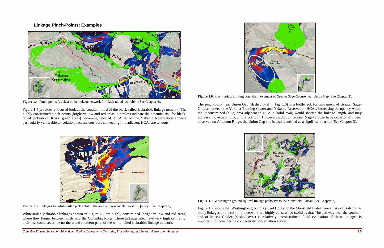
Linkage Pinch-Points: Examples

Figure 1.4. Pinch-points (circles) in the linkage network for black-tailed jackrabbit (See Chapter 4).

Figure 1.4 provides a focused look at the southern third of the black-tailed jackrabbit linkage network. The

highly constrained pinch-points (bright yellow and red areas in circles) indicate the potential risk for black-

tailed jackrabbit HCAs (green areas) becoming isolated. HCA 28 on the Yakama Reservation appears

particularly vulnerable to isolation because corridors connecting it to adjacent HCAs are tenuous.

Figure 1.5. Linkages for white-tailed jackrabbit in the area of Crescent Bar west of Quincy (See Chapter 5).

White-tailed jackrabbit linkages shown in Figure 1.5 are highly constrained (bright yellow and red areas)

where they funnel between cliffs and the Columbia River. These linkages also have very high centrality;

their loss could sever the northern and southern parts of the white-tailed jackrabbit linkage network.

Figure 1.6. Pinch-points limiting potential movement of Greater Sage-Grouse near Union Gap (See Chapter 3).

The pinch-point near Union Gap (dashed oval in Fig. 1.6) is a bottleneck for movement of Greater Sage-

Grouse between the Yakima Training Center and Yakama Reservation HCAs. Increasing occupancy within

the unconstrained (blue) area adjacent to HCA 7 (solid oval) would shorten the linkage length, and may

increase movement through the corridor. However, although Greater Sage-Grouse have occasionally been

observed on Ahtanum Ridge, the Union Gap site is also identified as a significant barrier (See Chapter 3).

Figure 1.7. Washington ground squirrel linkage pathways to the Mansfield Plateau (See Chapter 7).

Figure 1.7 shows that Washington ground squirrel HCAs on the Mansfield Plateau are at risk of isolation as

many linkages to the rest of the network are highly constrained (solid ovals). The pathway near the southern

end of Moses Coulee (dashed oval) is relatively unconstrained. Field evaluation of these linkages is

important for considering connectivity conservation action.


Barriers and Restoration Opportunities: Examples

Figure 1.8. Potential barriers to Townsend’s ground squirrel created by roads near the Hanford Site (See Chapter 6).

Arrows indicate barriers along SR 240 identified by the barrier/restoration opportunity analysis.

Figure 1.8 shows locations along the two-lane highway SR 240 that may create movement barriers for

Townsend’s ground squirrel on the Hanford Site. This location may provide a valuable opportunity to test

the barrier effect of highways for Townsend’s ground squirrel.

Figure 1.9. A natural barrier to tiger salamander movement created by the Columbia River (See Chapter 12).

Wide, deep-water areas such as the Columbia River (Fig. 1.9) with numerous predators may or may not

create complete barriers for salamander movements. Collection of genetic data could help determine the

strength of such barriers.

Figure 1.10. Barriers to movement of Western rattlesnake in the vicinity of Wenatchee (See Chapter 10).

Figure 1.10 indicates multiple opportunities for restoration (areas of yellow, red, and blue) in the ―triangle‖

connecting HCAs 31, 33, and 37. Multiple connections to HCA 39 may also have high restoration potential.

Roads create major movement barriers between HCAs 33 and 38, while increasing urban development

threatens linkages between HCAs 41 and 36.

Figure 1.11. Close-up of barriers along linkages for beavers in the area near Dry Falls, north of Ephrata (See Chapter

11). Panel ―a‖ depicts results of the barrier/restoration analysis overlaid on the aerial image. Panel ―b‖ shows the same

area without the barrier data. Arrows on both panels indicate an area traversed by a beaver linkage. Ovals indicate

steep cliffs which act as movement barriers.

Many identified barriers for beaver movement are created by natural landscape features such as steep terrain

and rocky areas. Figure 1.11a illustrates an identified barrier (area of yellow, red, and blue) in the linkage

between Banks Lake and the HCA in the vicinity of Ephrata. Parts of the linkage highlighted yellow

indicate areas that, if restored, would yield considerable improvement in connectivity for beavers. Figure

1.11b shows that the identified barrier consists of steep, rugged terrain which is not ―restorable.‖

(a) (b)


Focal Species Composites: Examples

Panel a. Columbia Plateau focal species. Panel b. The Ahtanum Ridge to Rattlesnake Hills linkage near Union Gap.

The dashed oval indicates the location of a substantial pinch-point and barrier

complex.

Panel c. Close-up view of the pinch-point / barrier (dashed oval); this barrier

location is identified by five species models. It includes the Yakima River,

railroad tracks, multiple highways, and agriculture.

Panel d. Composite linkage centrality analysis example. Yellow indicates the

composite centrality rating is Very High at this location. Panel e. Composite pinch-point analysis example. Red indicates four to five

focal species models identified this location as a strong pinch-point. Panel f. Composite barrier and restoration opportunities analysis example.

Yellow indicates sites that rate the Highest improvement score category based

on the summing of potential improvement scores across species.

Figure 1.12. Our composite maps integrate centrality, pinch-point, and barrier/restoration opportunity analysis results across all 11 focal species (Panels ―a‖ – ―f‖; See Chapter 13). Here we show the 11 focal species and illustrate results of some

of the composite analyses at the Ahtanum Ridge to Rattlesnake Hills linkage near Union Gap, an area which acts as both a pinch-point and barrier for several species. See page vi for species photo credits.

(a) (b) (c)

(d) (e) (f)

(c)

chapter 1. addendum overview: centrality, pinch-point, and

Documents