chapter 1 · 2008-07-29 · protein, one must ﬁnd a very speciﬁc setting of conditions (i.e.,...

Chapter 1

Machine Learning in StructuralBiology: Interpreting 3D ProteinImages

Frank DiMaio, Ameet Soni and Jude ShavlikUniversity of Wisconsin – Madison

1.1 Introduction . . . . . . . . . . . . . . . . . . . . . . . . . . . . . . . . . . . . . . . . . . . . . . . . . . . . . . . . . . . . . 11.2 Background . . . . . . . . . . . . . . . . . . . . . . . . . . . . . . . . . . . . . . . . . . . . . . . . . . . . . . . . . . . . . . 21.3 arp/warp . . . . . . . . . . . . . . . . . . . . . . . . . . . . . . . . . . . . . . . . . . . . . . . . . . . . . . . . . . . . . . . 111.4 resolve . . . . . . . . . . . . . . . . . . . . . . . . . . . . . . . . . . . . . . . . . . . . . . . . . . . . . . . . . . . . . . . . . . 151.5 textal . . . . . . . . . . . . . . . . . . . . . . . . . . . . . . . . . . . . . . . . . . . . . . . . . . . . . . . . . . . . . . . . . . . 221.6 acmi . . . . . . . . . . . . . . . . . . . . . . . . . . . . . . . . . . . . . . . . . . . . . . . . . . . . . . . . . . . . . . . . . . . . . 271.7 Conclusion . . . . . . . . . . . . . . . . . . . . . . . . . . . . . . . . . . . . . . . . . . . . . . . . . . . . . . . . . . . . . . . 36

1.1 Introduction

This chapter discusses an important problem that arises in structural bi-ology: given an electron density map – a three-dimensional “image” of aprotein produced from crystallography – identify the chain of protein atomscontained within the image. Traditionally, a human performs this interpreta-tion, perhaps aided by a graphics terminal. However, over the past 15 years,a number of research groups have used machine learning to automate den-sity map interpretation. Early methods had much success, saving thousandsof crystallographer-hours, but require extremely high-quality density mapsto work. Newer methods aim to automatically interpret poorer and poorerquality maps, using state-of-the-art machine learning and computer visionalgorithms.

This chapter begins with a brief introduction to structural biology and x-raycrystallography. This introduction describes in detail the problem of densitymap interpretation, a background on the algorithms used in automatic inter-pretation, and a high-level overview of automated map interpretation. Thechapter also describes four methods in detail, presenting them in chronolog-ical order of development. We apply each algorithm to an example densitymap, illustrating each algorithm’s intermediate steps and the resultant inter-pretation. Each algorithm’s section presents pseudocode and program flowdiagrams. The chapter concludes with a discussion of the advantages and

0-8493-0052-5/00/$0.00+$.50c© 2001 by CRC Press LLC 1

2

shortcomings of each method, as well as future research directions.

1.2 Background

Knowledge of a protein’s folding – that is, the sequence-determined three-dimensional structure – is valuable to biologists. A protein’s structure pro-vides great insight into the mechanisms by which a protein acts, and knowingthese mechanisms helps increase our basic understanding of the underlyingbiology. Structural knowledge is increasingly important in disease treatment,and has led to the creation of catalysts with industrial uses. No existingcomputer algorithm can accurately map sequence to 3D structure; however,several experimental “wet lab” techniques exist for determining macromole-cular structure. The most commonly used method, employed for about 80%of structures currently known, is x-ray crystallography. This time-consumingand resource-intensive process uses the diffraction pattern of x-rays off a crys-tallized matrix of protein molecules to produce an electron density map. Thiselectron density map is a three-dimensional “picture” of the electron cloudssurrounding each protein atom. Producing a protein structure is then a matterof identifying the location of each of the protein’s atoms in this 3D picture.

Density map interpretation – traditionally performed by a crystallographer– is time-consuming and, in noisy or poor-quality maps, often error-prone.Recently, a number of research groups have looked into automatically inter-preting electron density maps, using ideas from machine learning and com-puter vision. These methods have played a significant role in high-throughputstructure determination, allowing novel protein structures to quickly be elu-cidated.

1.2.1 Protein structure

Proteins (also called polypeptides) are constructed from a set of buildingblocks called amino acids. Each of the twenty naturally-occurring aminoacids consists of an amino group and a carboxylic acid group on one end,and a variable chain on the other. When forming a protein, adjacent aminogroups and carboxylic acid groups condense to form a repeating backbone(or mainchain), while the variable regions become dangling sidechains. Theatom at the interface between the sidechain and the backbone is known as thealpha carbon, or Cα for short (see Figure 1.1). The linear list of amino acidscomposing a protein is often referred to as the protein’s primary structure(see Figure 1.2a).

A protein’s secondary structure (see Figure 1.2b) refers to commonly oc-curring three-dimensional structural motifs taken by continuous segments in

Machine Learning in Structural Biology 3

H N

H

C

H

C

O

CH2

OH

N

H

C

H

C

O

CH

H3C

N

H

C

H

C

O

CH2

SH CH3

OH

Amino end (N-terminus)

Carboxyl end (C-terminus)

Peptide bond

Sidechains

Backbone

Alpha carbon

Amino acid residue

FIGURE 1.1: Proteins are constructed by joining chains of amino acids inpeptide bonds. A chain of three amino acid residues is illustrated.

(a)

(b)

(c) MET−SER−SER−SER−SER−SER−VAL−PRO−ALA−TYR−LEU−GLY−ALA−LEU−GLY−TYR−MET−ALA−MET−VAL−PHE−ALA−CYS−...

MET−SER−SER−SER−SER−SER−VAL−PRO−ALA−TYR−LEU−GLY−ALA−

LEU−GLY−TYR−MET−ALA−MET−VAL−PHE−ALA−CYS−...

FIGURE 1.2: An illustration of: (a) a protein’s primary structure, the linearamino-acid sequence of the protein, (b) a protein’s secondary structure, whichdescribes local structural motifs such as alpha helices and beta sheets, and(c) a protein’s tertiary structure, the global three-dimensional conformationof the protein.

the protein. There are two such motifs: α-helices, in which the peptide chainfolds in a corkscrew, and β-strands, where the chain stretches out linearly. Inmost proteins, several β-strands run parallel or antiparallel to one another.These regular structural motifs are connected by less-regular structures, calledloops (or turns). A protein’s secondary structure can be predicted somewhataccurately from its amino-acid sequence [1].

Finally, a protein’s three-dimensional conformation – also called its ter-tiary structure (see Figure 1.2c) – is uniquely determined from its aminoacid sequence (with some exceptions). No existing computer algorithm canaccurately map sequence to tertiary structure; instead, we must rely on ex-perimental techniques, primarily x-ray crystallography, to determine tertiarystructure.

4

Data collection

Phasing experiments

X-raydiffraction

FFT

Interpretation

NREFlections= 13624ANOMalous= FALSeDECLare NAME=IOBS DOMAin=RECIprocal TYPE=REAL ENDDECLare NAME=SIGI DOMAin=RECIprocal TYPE=REAL ENDDECLare NAME=FOBS DOMAin=RECIprocal TYPE=REAL ENDDECLare NAME=SIGMA DOMAin=RECIprocal TYPE=REAL ENDINDEx= 0 0 2 IOBS= 877.50 SIGI= 44.00 FOBS= 29.62 SIGMA= 0.75INDEx= 0 0 3 IOBS= 20114.70 SIGI= 994.60 FOBS= 141.83 SIGMA= 3.55INDEx= 0 0 4 IOBS= 17701.90 SIGI= 794.10 FOBS= 133.05 SIGMA= 3.02INDEx= 0 0 5 IOBS= 380.90 SIGI= 24.70 FOBS= 19.52 SIGMA= 0.64INDEx= 0 0 6 IOBS= 6762.20 SIGI= 266.70 FOBS= 82.23 SIGMA= 1.64INDEx= 0 0 7 IOBS= 2333.80 SIGI= 108.40 FOBS= 48.31 SIGMA= 1.14

0 0 2 29.62 0.00 0.00 0 0 3 141.83 0.00 0.00 0 0 4 133.05 0.00 0.00 0 0 5 19.52 0.00 0.00 0 0 6 82.23 0.00 0.00 0 0 7 48.31 0.00 0.00 0 0 8 73.36 0.00 0.00 0 0 9 108.23 0.00 0.00 0 0 10 160.50 0.00 0.00 0 0 11 4.77 0.00 0.00

Protein Crystal

Collection Plate

List of Phases

List of Reflections

Density Map

Protein Structure

FIGURE 1.3: An overview of the crystallographic process.

1.2.2 X-ray crystallography

An overview of protein crystallography appears in Figure 1.3. Given asuitable target for structure determination, a crystallographer must produceand purify this protein in significant quantities. Then, for this particularprotein, one must find a very specific setting of conditions (i.e., pH, solventtype, solvent concentration) under which protein crystals will form. Once asatisfactory crystal forms, it is placed in front of an x-ray source. Here, thiscrystal diffracts a beam of x-rays, producing a pattern of spots on a collector.These spots – also known as reflections or structure factors – represent theFourier-transformed electron density map. Unfortunately, the experiment canonly measure the intensities of these (complex-valued) structure factors; thephases are lost.

Determining these missing phases is known as the phase problem in crys-tallography, and can be solved to a reasonable approximation using compu-tational or experimental techniques [2]. Only after estimating the phases canone compute the electron-density map (which we will refer to as a “densitymap” or simply “map” for short).

The electron density map is defined on a 3D lattice of points covering theunit cell, the basic repeating unit in the protein crystal. The crystal’s unitcell may contain multiple copies of the protein related by crystallographicsymmetry, one of the 65 regular ways a protein can pack into the unit cell.Rotation/translation operators relate one region in the unit cell (the asym-metric unit) to all other symmetric copies. Furthermore, the protein may forma multimeric complex (e.g. a dimer, tetramer, etc.) within the asymmetricunit. In all these cases is up to the crystallographer to isolate and interpret asingle copy of the protein.

Figure 1.4 shows a sample fragment from an electron density map, andthe corresponding interpretation of that fragment. The amino-acid (primary)sequence of the protein is typically known by the crystallographer before in-terpreting the map. In a high-quality map, every single (non-hydrogen) atomin the protein can be placed in the map (Figure 1.4b). In a poor-quality map


(a) (c)(b)

FIGURE 1.4: An overview of electron density map interpretation. Giventhe amino-acid sequence of the protein and a density map (a), the crystallogra-pher’s goal is to find the positions of all the protein’s atoms (b). Alternatively,a backbone trace (c), represents each residue by its Cα location.

1Å 2Å 3Å 4Å 5Å

FIGURE 1.5: Electron density map quality at various resolutions. The“sticks” show the position of the atoms generating the map.

it may only be possible to determine the general locations of each residue.This is known as a Cα trace (Figure 1.4c). This information - though not ascomprehensive as an all-atom model - is still valuable to biologists.

The quality of experimental maps as well as the sheer number of atomsin a protein makes interpretation difficult. Certain protein crystals producea very narrow diffraction pattern, resulting in a poor-quality, “smoothed”density map. This is quantified as the resolution of a density map, a numericvalue which refers to the minimum distance at which two peaks in the densitymap can be resolved. Figure 1.5 shows a simple density map at a variety ofresolutions.

Experimentally determined phases are often very inaccurate, and make in-terpretation difficult as well. As the model is built, these phases are iterativelyimproved [3], producing a better quality map, which may require resolvinglarge portions of the map. Figure 1.6 illustrates the effect poor phasing hason density-map quality. In addition, noise in diffraction-pattern data collec-tion also introduces errors into the resulting density map.

Finally, the density map produced from x-ray crystallography is not an

6

least noise most noise

FIGURE 1.6: Electron density map quality as noise is added to the com-puted phases. The “sticks” show the position of the atoms generating themap.

“image” of a single molecule, but rather an average over an ensemble of allthe molecules contained within a single crystal. Flexible regions in the proteinare not visible at all, as they are averaged out.

For most proteins, this interpretation is done by an experienced crystal-lographer, who can, with high-quality data, fit about 100 residues per day.However, for poor-quality structures or structures with poor phasing, interpre-tation can be an order of magnitude slower. Consequently, map interpretationis the second-most time-consuming step in the crystallographic process (aftercrystal preparation).

A key question for computational methods for interpreting density maps isthe following: how are candidate 3D models scored? Crystallographers typ-ically use a model’s R-factor (for residual index ) to evaluate the quality ofan interpretation. Formally, the R-factor is defined, given experimentally de-termined structure factors Fobs and model-determined structure factors Fobs,as:

R =∑||Fobs| − |Fcalc||∑

|Fobs|(1.1)

The R-factor measures how well the proposed 3D structure explains theobserved electron-density data. Crystallographers usually strive to get R-factors under 0.2 (or lower, depending on map resolution), while also buildinga physically-feasible (i.e. valid bond distances, torsion angles, etc.) proteinmodel without adding too many water molecules. One can always reduce theR-factor by placing extra water molecules in the density map; these reductionsare a result overfitting the model to the data, and don’t correspond to aphysically feasible interpretation.

Another commonly used measure is free R-factor, or Rfree. Here, 5-10%of reflections are randomly held out as a test set before refinement. Rfree

is the R-factor for these held-aside reflections. Using Rfree tends to avoidoverfitting the protein’s atoms to the reflection data.


1.2.3 Algorithmic background

Algorithms for automatically interpreting electron density maps draw heav-ily from the machine learning and statistics communities. These communitieshave developed powerful frameworks for modeling uncertainty, reasoning fromprior examples, and statistically modeling data, all of which have been usedby researchers in crystallography. This section briefly describes the statistaland machine learning methods used by the interpretation methods presentedin this paper. This section is intended as a basic introduction to these topics.Interested readers should consult Russell and Norvig’s text [4] or Mitchell’stext [5] for a thorough overview.

1.2.3.1 Probabilistic models

A model here refers to a system that simulates a real-world event or process.Probabilistic models simulate uncertainty by producing different outcomeswith different probabilities. In such models, the probabilities associated withcertain events is generally not known, and instead has to be estimated froma training set, a set of previously solved problem instances. Using maximumlikelihood estimation, the probability of a particular outcome is estimated asthe frequency at which that outcome occurs in the training set.

The unconditional or prior probability of some outcome A is denoted P (A).Assigning some value to this probability, say P (A) = 0.3, means that inthe absence of any other information, the best assignment of probability ofoutcome A is 0.3. As an example, when flipping a (fair) coin, P (“heads”) =0.5. In this section, we use “outcome” to mean the setting of some randomvariable; P (X = xi) is the probability that variable X takes value xi. We willuse the shorthand P (xi) to refer to this same value.

The conditional or posterior probability is used when other, previously un-known, information becomes available. If other information, B, relevant toevent A is known, then the best assignment of probability to event A is givenby the conditional P (A|B). This reads “the probability of A, given B.”If more evidence, C, is uncovered, then the best probability assignment isP (A|B,C) (where “,” denotes “and”).

The joint probability of two or more events is the probability of both eventsoccurring, and – for two events A and B – is denoted P (A,B) and is read“the probability of A and B”. Conditional and joint probabilities are relatedusing the expression:

P (A,B) = P (A|B)P (B) = P (B|A)P (A) (1.2)

This relation holds for any events A and B. Two events are independentif their joint probability is the same as the product of their unconditionalprobabilities, P (A,B) = P (A)P (B). If A and B are independent we alsohave P (A|B) = P (A), that is, knowing B tells us nothing about A.

One computes the marginal probability by taking the joint probability andsumming out one or more variables. That is, given the joint distribution

8

P (A,B,C), one computes the marginal distribution of A as:

P (A) =∑B

∑C

P (A,B,C) (1.3)

Above, the sums are over all possible outcomes of events B and C. The mar-ginal distribution is important because it provides information about the dis-tribution of some variables (A above) in the full joint distribution, withoutrequiring one to explicitly compute the (possibly intractable) full joint distri-bution.

Finally, Bayes’ rule allows one to reverse the direction of a conditional:

P (A|B) =P (B|A)P (A)

P (B)(1.4)

Bayes’ rule is useful for computing a conditional P (A|B) when direct esti-mation (using frequencies from a training set) is difficult, but when P (B|A)can be estimated accurately. Often, one drops the denominator, and insteadcomputes the relative likelihood of two outcomes, for example, P (A = a1|B)versus P (A = a2|B). If a1 and a2 are the only possible outcomes for A, thenexact probabilities can be determined by normalization; there is no need tocompute the prior P (B).

1.2.3.2 Case-based reasoning

Broadly defined, case-based reasoning (CBR) attempts to solve a new prob-lem by using solutions to similar past problems. Algorithms for case-basedreasoning require a database of previously solved problem instances, andsome distance function to calculate how “different” two problem instancesare. There are two key aspects of CBR systems. First, learning in such sys-tems is lazy : the models only generalize to unseen instances when presentedwith such a new instance. Second, they only use instances “close” to theunseen instance when categorizing it.

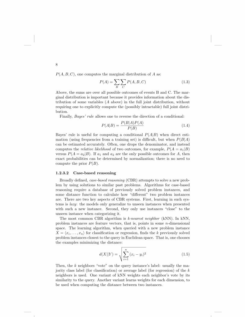
The most common CBR algorithm is k-nearest neighbor (kNN). In kNN,problem instances are feature vectors, that is, points in some n-dimensionalspace. The learning algorithm, when queried with a new problem instanceX = 〈xi, . . . , xn〉 for classification or regression, finds the k previously solvedproblem instances closest to the query in Euclidean space. That is, one choosesthe examples minimizing the distance:

d(X||Y ) =

√√√√ n∑i=1

(xi − yi)2 (1.5)

Then, the k neighbors “vote” on the query instance’s label: usually the ma-jority class label (for classification) or average label (for regression) of the kneighbors is used. One variant of kNN weights each neighbor’s vote by itssimilarity to the query. Another variant learns weights for each dimension, tobe used when computing the distance between two instances.


Σ Σ

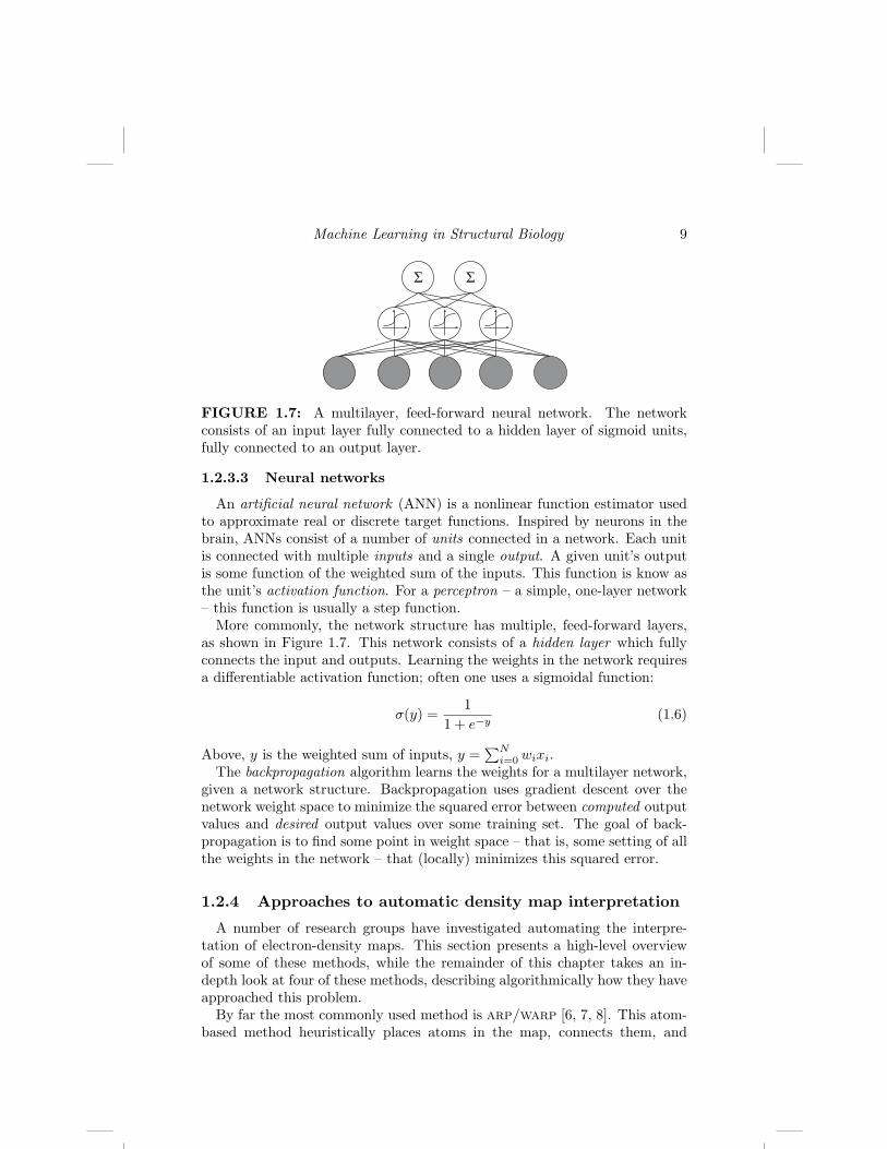
FIGURE 1.7: A multilayer, feed-forward neural network. The networkconsists of an input layer fully connected to a hidden layer of sigmoid units,fully connected to an output layer.

1.2.3.3 Neural networks

An artificial neural network (ANN) is a nonlinear function estimator usedto approximate real or discrete target functions. Inspired by neurons in thebrain, ANNs consist of a number of units connected in a network. Each unitis connected with multiple inputs and a single output. A given unit’s outputis some function of the weighted sum of the inputs. This function is know asthe unit’s activation function. For a perceptron – a simple, one-layer network– this function is usually a step function.

More commonly, the network structure has multiple, feed-forward layers,as shown in Figure 1.7. This network consists of a hidden layer which fullyconnects the input and outputs. Learning the weights in the network requiresa differentiable activation function; often one uses a sigmoidal function:

σ(y) =1

1 + e−y(1.6)

Above, y is the weighted sum of inputs, y =∑N

i=0 wixi.The backpropagation algorithm learns the weights for a multilayer network,

given a network structure. Backpropagation uses gradient descent over thenetwork weight space to minimize the squared error between computed outputvalues and desired output values over some training set. The goal of back-propagation is to find some point in weight space – that is, some setting of allthe weights in the network – that (locally) minimizes this squared error.

1.2.4 Approaches to automatic density map interpretation

A number of research groups have investigated automating the interpre-tation of electron-density maps. This section presents a high-level overviewof some of these methods, while the remainder of this chapter takes an in-depth look at four of these methods, describing algorithmically how they haveapproached this problem.

By far the most commonly used method is arp/warp [6, 7, 8]. This atom-based method heuristically places atoms in the map, connects them, and

10

refines their positions. To handle poor phasing, arp/warp uses an iterativealgorithm, consisting of alternating phases in which (a) a model is built froma density map, and (b) the density map’s phases are improved using theconstructed model. This algorithm is widely used, but has one drawback:fairly high resolution data, about 2.3A or better, is needed. Given this high-resolution data, the method is extremely accurate; however, many proteincrystals fail to diffract to this extent.

Several approaches represent the density map in an alternate form, in theprocess making the map more easily interpretable for both manual and au-tomated approaches. One of the earliest such methods, skeletonization, wasproposed for use in protein crystallography by Greer’s bones algorithm [9].Skeletonization, similar to the medial-axis transformation in computer vision,gradually thins the density map until it is a narrow ribbon approximatelytracing the protein’s backbone and sidechains. More recent work by Leherteet al. [10], represents the density map as an acyclic graph: a minimum span-ning tree connecting all the critical points (points where the gradient of thedensity is 0) in the electron density map. This representation accurately ap-proximates the backbone with 3A or better data, and separates protein fromsolvent up to 5A resolution.

Cowtan’s fffear efficiently locates rigid templates in the density map [11].It uses fast Fourier transforms (FFTs) to quickly match a learned templateover all locations in a density map. Cowtan provides evidence showing it lo-cates alpha helices in poorly-phased 8A maps. Unfortunately, the techniqueis limited in that in can only locate large rigid templates (e.g. those corre-sponding to secondary-structure elements). One must trace loops and mapthe fit to the sequence manually. However, a number of methods use fffearas a template-matching subroutine in a larger interpretation algorithm.

X-autofit, part of the quanta [12] package, uses a gradient refinementalgorithm to place and refine the protein’s backbone. Their refinement takesinto account the density map as well as bond geometry constraints. Theyreport successful application of the method at resolutions ranging from 0.8 to3.0A.

Terwilliger’s resolve contains an automated model-building routine [13,14] uses a hierarchical procedure in which helices and strands are located andfitted, then are extended in an iterative fashion, using a library of tripeptides.Finally, resolve applies a greedy fragment-merging routine to overlappingextended fragments. The approach was able to place approximately 50% ofthe protein chain in a 3.5A resolution density map.

Levitt’s maid [15] approaches map interpretation “as a human would,” byfirst finding the major secondary structures, alpha helices and beta sheets,connecting the secondary-structure elements, and mapping this fit to the pro-vided sequence. Maid reports success on density maps at around 2.8A reso-lution.

Ioerger’s textal [16, 17, 18] attempts to interpret poor-resolution (2.2 to3.0A) density maps using ideas from pattern recognition. Ioerger constructs


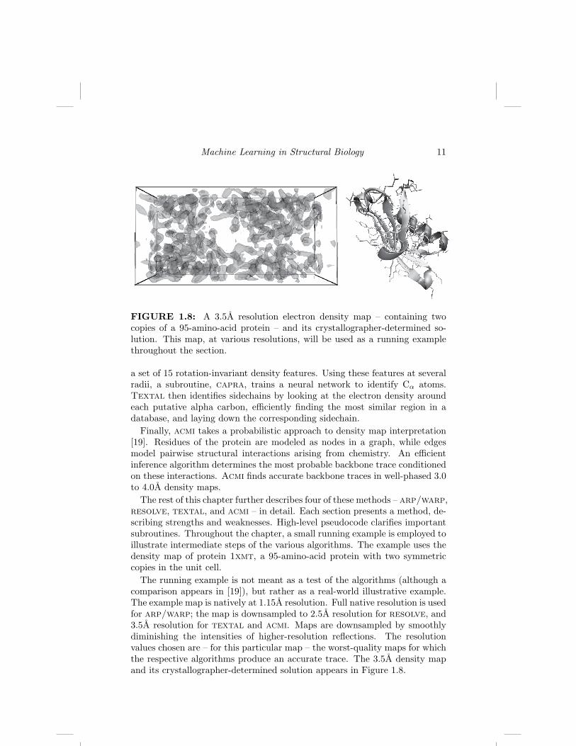
FIGURE 1.8: A 3.5A resolution electron density map – containing twocopies of a 95-amino-acid protein – and its crystallographer-determined so-lution. This map, at various resolutions, will be used as a running examplethroughout the section.

a set of 15 rotation-invariant density features. Using these features at severalradii, a subroutine, capra, trains a neural network to identify Cα atoms.Textal then identifies sidechains by looking at the electron density aroundeach putative alpha carbon, efficiently finding the most similar region in adatabase, and laying down the corresponding sidechain.

Finally, acmi takes a probabilistic approach to density map interpretation[19]. Residues of the protein are modeled as nodes in a graph, while edgesmodel pairwise structural interactions arising from chemistry. An efficientinference algorithm determines the most probable backbone trace conditionedon these interactions. Acmi finds accurate backbone traces in well-phased 3.0to 4.0A density maps.

The rest of this chapter further describes four of these methods – arp/warp,resolve, textal, and acmi – in detail. Each section presents a method, de-scribing strengths and weaknesses. High-level pseudocode clarifies importantsubroutines. Throughout the chapter, a small running example is employed toillustrate intermediate steps of the various algorithms. The example uses thedensity map of protein 1xmt, a 95-amino-acid protein with two symmetriccopies in the unit cell.

The running example is not meant as a test of the algorithms (although acomparison appears in [19]), but rather as a real-world illustrative example.The example map is natively at 1.15A resolution. Full native resolution is usedfor arp/warp; the map is downsampled to 2.5A resolution for resolve, and3.5A resolution for textal and acmi. Maps are downsampled by smoothlydiminishing the intensities of higher-resolution reflections. The resolutionvalues chosen are – for this particular map – the worst-quality maps for whichthe respective algorithms produce an accurate trace. The 3.5A density mapand its crystallographer-determined solution appears in Figure 1.8.

12

electron density map

Place free atoms into map

Join chains of free atoms (autotrace)

Refine model using connectivity constraints

Trace sidechains

free atoms model

hybrid model

complete backbone model

hybridmodel

complete all-atom model

FIGURE 1.9: A flowchart of warpntrace.

1.3 arp/warp

The arp/warp (automated refinement procedure) software suite is a crys-tallographic tool for the interpretation and refinement of electron densitymaps. Arp/warp’s warpntrace procedure was the first automatic inter-pretation tool successfully used for protein models. Today, it remains one ofthe most used tools in the crystallographic community for 3D protein-imageinterpretation. Arp/warp concentrates on the best placement of individualatoms in the map: no attempt is made to identify higher-order constructs likeresidues, helices, or strands. Arp/warp’s “atom-level” method requires high-quality data, however. In general, arp/warp requires maps at a resolutionof 2.3A or higher to produce an accurate trace.

Figure 1.9 illustrates an overview of warpntrace. Warpntrace beginsby creating a free atom model – a model containing only unconnected atoms– to fill in the density map of the protein. It then connects some of theseatoms using a heuristic, creating a hybrid model. This hybrid model con-sists of a partially-connected backbone, together with a set of unconstrainedatoms. This hybrid model is refined, producing a map with improved phaseestimates. The process iterates using this improved map. At each iteration,warpntrace removes every connection, restarting with a free-atom model.

1.3.1 Free-atom placement

Arp/warp contains a atom placement method based on arp, an interpre-tation method for general molecular models. Arp randomly places uncon-nected atoms into the density map, producing a free atom model, illustratedin Figure 1.10a. To initialize the model, arp begins with a small set of atomsin the density map. It slowly expands this model by looking for areas abovea density threshold, at a bonding distance away from existing atoms. The


(c)

(a)

(b)

FIGURE 1.10: Intermediate steps in arp/warp’s structure determination:(a) the free atom model, where waters are placed in the map, (b) the hybridmodel, after some connections are determined, and (c) the final determinedstructure.

density threshold is slowly lowered until arp places the desired number offree atoms.

For small molecules, arp’s next step is refining the free-atom model; that is,iteratively moving atoms to better explain the density map. Free-atom refine-ment ignores stereochemical information, and moves each atom independentlyto produce a complete structure. Arp’s free-atom refinement, in addition tomoving atoms, considers adding or removing atoms from the model. Multiplerandomized initial structures are used to improve robustness. Further detailsare available from Perrakis et al. [7].

However, with molecules as large as proteins, free-atom refinement alone isinsufficient to produce an accurate model. Performing free-atom refinementwith tens of thousands of atoms leads to overfitting, producing a model that isnot physically feasible. For determining protein structures, arp/warp makesuse of connectivity information in its refinement, using free-atom placement asa starting point. The procedure warpntrace adds connectivity informationto the free atom model.

14

ALGORITHM 1.1: Warpntrace’s model-building algorithmGiven: electron density map M, free-atom model F, sequence seqFind: all-atom model

for i = 1 to nIterations doH← F // initialize hybrid modelCA pairs← highest-scoring atom pairs 3.8± 0.5A apartforeach ci ∈ CA pairs do

if (ci does not match backbone template) thendelete ci from CA pairs

endend

while a Cα chain of length ≥ 5 remains in CA pairs dobestChain← longest fragment in DB overlapping CA pairsremove bestChain’s atoms from CA pairs, Hadd bestChain to H

endH′ ← refine(H)F← remove connections from hybrid model H′

endmodel← sidechainTrace(H′)

1.3.2 Main-chain tracing

Given a free-atom model of a protein, one can form a crude backbone traceby looking for pairs of free atoms the proper distance apart. Warpntraceformalizes this procedure, called autotracing, using a heuristic method. Themethod is outlined in Algorithm 1.1. Warpntrace assigns a score – basedon density values – to each free atom. The highest scoring atom pairs 3.8 ±0.5A apart become candidate Cα’s. The algorithm verifies candidate pairs byoverlaying them with a peptide template. If the template matches the map,warpntrace saves the candidate pair.

After computing a list of Cα pairs, warpntrace constructs the backboneusing a database of known backbone conformations (taken from solved proteinstructures). Given a chain of candidate Cα pairs, warpntrace considers allbackbone conformations in the database with matching Cα positions, orderedby length. The longest candidate backbone is then added to the model. Thealgorithm connects the corresponding free atoms, and removes these atomsfrom the free-atom pool. The process repeats as long as there remain candi-date Cα chains at least 5 residues in length.

Autotracing produces a hybrid model, shown in Figure 1.10b. A hybridmodel contains a set of connected chains together with a set of free atoms.Autotracing identifies some atom types and connectivity, which enables theuse of some stereochemical information in refinement. Added restraints in-crease the number of observations available, and increase the probability of


producing a good model. The tracing is initially very conservative, with manyfree atoms remaining in the model. Adding too many restraints too early leadsto overfitting the model.

Finally, a modified version of arp refines this hybrid model. Arp uses therefined structure to improve the experimentally determined phases, makingthe map clearer to interpret. At each iteration of this “autotrace–refine–recompute phases” cycle, warpntrace returns to a free-atom model, by re-moving previous traces. Since the map is better-phased, autotracing producesa more complete model. This, in turn, provides a better refinement, improvingthe phases further.

This cycle continues for a fixed number of iterations, or until a completetrace is available. Finally, warpntrace adds on side-chains by identifyingpatterns of free atoms around Cα’s. It aligns these free-atom patterns to thesequence to produce a complete model. Figure 1.10c illustrates the completearp/warp-determined trace on the running example.

1.3.3 Discussion

Arp/warp is the preferred method for automatically interpreting elec-tron density maps, assuming sufficiently high-resolution data is available. Itsplacement of individual atoms, followed by atom-level refinement, producesan extremely accurate trace with no user action required in 2.3A or betterdensity maps. It is widely used by crystallographers to rapidly construct aprotein model. Unfortunately, many protein crystals fail to produce maps ofsufficient quality, and one must consider alternate methods.

1.4 resolve

While arp/warp is extremely accurate with high-resolution data, manyprotein crystals fail to diffract to a sufficient level for accurate interpreta-tion. In general, arp/warp requires individual atoms to be visible in thedensity map, which happens at about 2.3A resolution or better. The nextthree methods – resolve, textal, and acmi – all aim to solve maps with> 2.3A resolution. All three methods take different approaches to the prob-lem; however, all three – in contrast to arp/warp – consider higher-levelconstructs than atoms when building a protein model. This allows accurateinterpretation even when individual atoms are not visible.

Resolve is a method developed by Terwilliger for automated model-buildingin poor-quality (around 3A) electron density maps [13, 14]. Figure 1.11 out-lines the complete hierarchical approach. Resolve’s method hinges upon theconstruction of two model secondary structure fragments – a short α-helix and

16


Identify helix/strand template matches

Extend matches iteratively

Assemble chain from fragments

Trace sidechains

helix/strand list

protein fragment list

backbone model

partialmodel


FIGURE 1.11: A flowchart of Resolve.

FIGURE 1.12: The averaged helix (left) and strand (right) fragment usedin resolve’s initial matching step.

β-strand – for the initial matching. Resolve first searches over all of rotationand translation space for these fragments; after placing a small set of over-lapping model fragments into the map, the algorithm considers a much largertemplate set as potential extensions. Resolve joins overlapping fragmentsand, finally, identifies sidechains corresponding to each Cα – conditioned onthe input sequence – and places individual atoms into the model.

1.4.1 Secondary structure search

Given an electron density map, resolve begins its interpretation by search-ing all translations and rotations in the map for a model 6-residue α-helix anda model 4-residue β-strand. Resolve constructs these fragments by aligninga collection of helices (or strands) from solved structures; it computes theelectron density for each at 3A resolution, and averages the density acrossall examples. The “average” models used by resolve are illustrated in Fig-ure 1.12.

Given these model fragments, resolve considers placing them at each po-sition in the map. At each position it considers all possible rotations (ata 30◦ or 40◦ discretization) of the fragment, and computes a standardizedsquared-density difference between the fragment’s electron density and the


(a)

(b)

(c)

FIGURE 1.13: Intermediate steps in resolve’s structure determination:(a) locations in the map that match short helical/strand fragments (b) thesame fragments after refinement and extension, and (c) the final determinedstructure.

map:

t(~x) =∑

~y

εf (~y)(ρ′f (~y)− 1

σf (~x)[ρ(~y − ~x)− ρ(~x)

])(1.7)

Above, ρ(~x) is the map in which we are searching, ρ′f (~x) is the standardizedfragment electron density, εf (~x) is a masking function that is nonzero onlyfor points near the fragment, and ρ(~x) and σf (~x) standardize the map in themasked region εf centered at ~x:

ρ(~x) =

∑~y εf (~y)ρ(~y − ~x)∑

~y εf (~y)

σ2f (~x) =

∑~y εf (~y)

[ρ(~y − ~x)− ρ(~x)

]2∑~y εf (~y)

(1.8)

Resolve computes the matching function t(~x) quickly over the entire unitcell using fffear’s FFT-based convolution [11].

After matching the two model fragments using a coarse rotational step-size,the method generates a list of best-matching translations and orientations of

18

each fragment (shown in Figure 1.13a). Processing these matches in order,Resolve refines each fragment’s position and rotation to maximize the real-space correlation coefficient (RSCC) between template and map:

RSCC(ρf , ρ) =〈ρf · ρ〉 − 〈ρf 〉〈ρ〉√

〈ρ2f 〉 − 〈ρf 〉2

√〈ρ2〉 − 〈ρ〉2

(1.9)

Here, 〈ρ〉 indicates the map mean over a fragment mask. Resolve onlyconsiders refined matches with an RSCC above some threshold.

1.4.2 Iterative fragment extension

At this point, resolve has a set of putative helix and strand locationsin the density map. The next phase of the algorithm extends these using amuch larger library of fragments, producing a model like that in Figure 1.13b.Specifically, resolve makes use of four such libraries for fragment extension:

(a) 17 α-helices between 6 and 24 amino acids in length

(b) 17 β-strands between 4 and 9 amino acids in length

(c) 9,232 tripeptides containing backbone atoms only for N-terminus exten-sion

(d) 4,869 tripeptides containing a partial backbone (the chain Cα − C −Owith no terminal N) plus two full residues for C-terminus extension

Resolve learns these fragment libraries from a set of previously solved proteinstructures. It constructs the two tripeptide libraries by clustering a largerdataset of tripeptides.

1.4.2.1 α-helix/β-strand extension

For each potential model’s placement in the map, resolve consider ex-tending it using each fragment in either set (a), if the model fragment is ahelix, or set (b), if the model fragment is a strand. For each fragment, re-solve chooses the longest segment of the fragment such that every atom inthe fragment has a density value above some threshold.

To facilitate comparison between these 17 segments of varying length (onefor each fragment in the library), each matching segment is given a scoreQ = 〈ρ〉

√N , with 〈ρ〉 the mean atom density, and N the number of atoms.

The algorithm computes a Z-score:

Z =Q− 〈Q〉σ(Q)

(1.10)

Resolve only considers segments with Z > 0.5. Notice there may be a largenumber of overlapping segments in the model at this point.


1.4.2.2 Loop extension using tripeptide libraries

For each segment in the model, resolve attempts to extend the segmentin both the N-terminal and C-terminal direction using the tripeptide library.Resolve tests each tripeptide in the library by superimposing the first residueof the tripeptide on the last residue of the current model segment. It thentests the top scoring “first-level” fragments for overlap (steric clashes) with thecurrent model segment. For those with no overlap, a lookahead step considersthis first-level extension as a starting point for a second extension. The scorefor each first-level extension is:

scorefirst-level = 〈ρfirst-level〉+ maxsecond-level

〈ρsecond-level〉 (1.11)

Above, 〈ρfirst-level〉 denotes the average map density at the atoms of the first-level extension.

Resolve accepts the best first-level extension – taking the lookahead terminto account – only if the average density is above some threshold densityvalue. If the density is too low, and the algorithm rejects the best fragment,several “backup procedures” consider additional first-level fragments, or step-ping back one step in the model segment. If these backup procedures fail,resolve rejects further extensions.

1.4.3 Chain assembly

Given this set of candidate model segments, resolve’s next step is assem-bling a continuous chain. To do so, it uses an iterative method, illustrated inAlgorithm 1.2. The outermost loop repeats until no more candidate segmentsremain. At each iteration, the algorithm chooses the top-scoring candidatesegment not overlapping any others. It considers all other segments in themodel as extensions: if at least two Cα’s between the candidate and extensionoverlap, then resolve accepts the extension. Finally, the extension becomesthe current candidate chain.

1.4.4 Sidechain trace

Resolve’s final step is, given a set of Cα positions in some density map, toidentify the corresponding residue type, and to trace all the sidechain atoms[14]. This sidechain tracing is the first time that resolve makes use of theanalyzed protein’s sequence. Resolve’s sidechain tracing uses a probabilisticmethod, finding the most likely layout conditioned on the input sequence.Resolve’s sidechain tracing procedure is outlined in Algorithm 1.3.

Resolve’s sidechain tracing relies on a rotamer library. This library con-sists of a set of low-energy conformations – or rotamers – that characterizeseach amino-acid type. Resolve builds a rotamer library from the sidechainsin 574 protein structures. Clustering produces 503 different low-energy side-

20

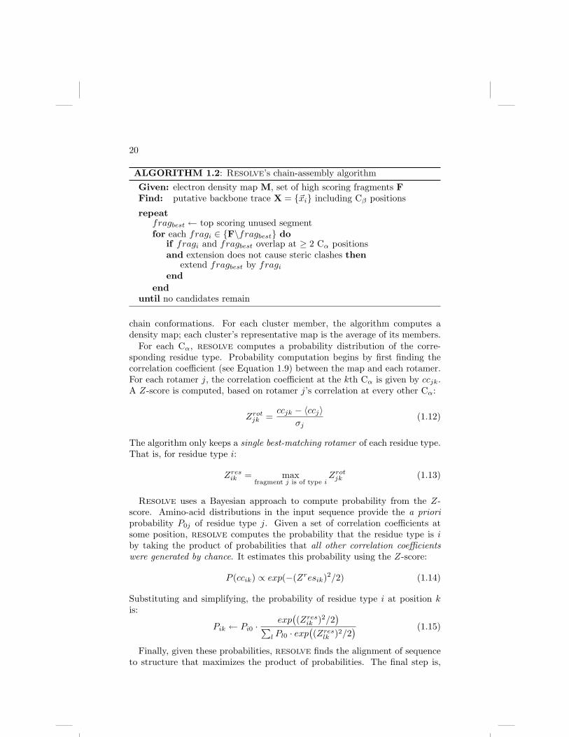
ALGORITHM 1.2: Resolve’s chain-assembly algorithmGiven: electron density map M, set of high scoring fragments FFind: putative backbone trace X = {~xi} including Cβ positions

repeatfragbest ← top scoring unused segmentfor each fragi ∈ {F\fragbest} do

if fragi and fragbest overlap at ≥ 2 Cα positionsand extension does not cause steric clashes then

extend fragbest by fragi

endend

until no candidates remain

chain conformations. For each cluster member, the algorithm computes adensity map; each cluster’s representative map is the average of its members.

For each Cα, resolve computes a probability distribution of the corre-sponding residue type. Probability computation begins by first finding thecorrelation coefficient (see Equation 1.9) between the map and each rotamer.For each rotamer j, the correlation coefficient at the kth Cα is given by ccjk.A Z-score is computed, based on rotamer j’s correlation at every other Cα:

Zrotjk =

ccjk − 〈ccj〉σj

(1.12)

The algorithm only keeps a single best-matching rotamer of each residue type.That is, for residue type i:

Zresik = max

fragment j is of type iZrot

jk (1.13)

Resolve uses a Bayesian approach to compute probability from the Z-score. Amino-acid distributions in the input sequence provide the a prioriprobability P0j of residue type j. Given a set of correlation coefficients atsome position, resolve computes the probability that the residue type is iby taking the product of probabilities that all other correlation coefficientswere generated by chance. It estimates this probability using the Z-score:

P (ccik) ∝ exp(−(Zresik)2/2) (1.14)

Substituting and simplifying, the probability of residue type i at position kis:

Pik ← Pi0 ·exp

((Zres

ik )2/2)∑

l Pl0 · exp((Zres

lk )2/2) (1.15)

Finally, given these probabilities, resolve finds the alignment of sequenceto structure that maximizes the product of probabilities. The final step is,


ALGORITHM 1.3: Resolve’s sidechain-placement algorithmGiven: map M, backbone trace X = {~xi} (including Cβ ’s),

sidechain library F, sequence seqFind: all-atom protein model

for each sidechain fj ∈ F dofor each Cα ~xk ∈ X do

ccjk ← RSCC(M(~xk), fj)) // see Equation 1.9Zjk ← (ccjk − 〈ccj〉)/σj

endend

// Estimate probabilities Pik that residue type i is at position kfor each residue type i do

Pi0 ← a priori distribution of residue type iZik ← max

fragment j of type iZjk

for each alpha carbon ~xk ∈ X doPik ← Pi0 · exp(Z2

ik/2)P

l Pl0·exp(Z2lk/2)

endend

// Align trace to sequence, place individual atomsalign seq to chains maximizing product of Pik’sif (good alignment exists) then

place best-fit sidechain of alignment-determined type at each positionend

given an alignment-determined residue type at each position, placing the ro-tamer of the correct type with the highest correlation coefficient Z-score. Re-solve’s final computed structure on the running example, both backbone andsidechain, is illustrated in Figure 1.13c.

1.4.5 Discussion

Unlike arp/warp, resolve uses higher-order constructs than individualatoms in tracing a protein’s chain. Searching for helices and strands in themap lets resolve produce accurate traces in poor-quality maps, in whichindividual atoms are not visible. This method is also widely used by crystal-lographers. Resolve has been successfully used to provide a full or partialinterpretation at maps with as poor as 3.5A resolution. Because the methodis based on heuristics, when map quality gets worse, the heuristics fail and theinterpretation is poor. Typically, the tripeptide extension is the first heuris-tic to fail, resulting in resolve traces consisting of disconnected secondarystructure elements. In poor maps, as well, resolve is often unable to iden-

22

tify sidechain types. However, resolve is able to successfully use backgroundknowledge from structural biology in order to improve interpretation in poor-quality maps.

1.5 textal

Textal – another method for density map interpretation – was developedby Ioerger et al. Much like resolve, textal seeks to expand the limit ofinterpretable density maps to those with medium to low resolution (2 to 3A).The heart of textal lies in its use of computer vision and machine learningtechniques to match patterns of density in an unsolved map against a data-base of known residue patterns. Matching two regions of density, however, isa costly six-dimensional problem. To deal with this, textal uses of a set ofrotationally invariant numerical features to describe regions of density. Theelectron density around each point in the map is converted to a vector of 19features sampled at several radii that remain constant under rotations of thesphere. The vector consists of descriptors of density, moments of inertia, sta-tistical variation, and geometry. Using rotationally invariant features allowsfor efficiency in determination – reducing the problem from 6D to 3D – andbetter generalization of patterns of residues.

Textal’s algorithm – outlined in Figure 1.14 – attempts to replicate theprocess by which crystallographers identify protein structures. The first stepis to identify the backbone – the location of each Cα – of the protein. Tracingthe backbone is done by capra (C-Alpha Pattern Recognition Algorithm),which uses a neural network to estimate each subregion’s distance to theclosest Cα given the rotationally invariant features discussed above. Capra’sputative Cα locations are then sent into the second part of the algorithm,lookup, which identifies the sidechains corresponding to each Cα’s. Lookupuses these same rotationally invariant features, but instead uses a nearestneighbor approach to find a small subset of the database that best matchesthe region of unknown density. Lookup rotationally aligns the best matchto the unknown residue, and places the corresponding atoms into the map.Finally, textal cleans up its trace using a set of post-processing routines.

1.5.1 Feature extraction

The most important component of textal is its extraction of a set of nu-merical features from a region of density. These numerical features allowrapid identification of similar regions from different (solved) maps. A key as-pect of textal’s feature set is invariance to arbitrary rotations of the region’sdensity. This eliminates the need for an expensive rotational search for each



Skeletonize density map

Extract rotation-invariant features

Identify Cα’s using a trained neural network

Trace sidechains

pseudo-atom list

feature vector list

backbone model


Build, patch, and stitch chains

predicted distances to Cα

FIGURE 1.14: A flowchart of textal.

fragment; additionally, a discrete rotational search is likely to underestimatesome match scores if the true rotation falls between rotational samples.

Textal uses 76 such numerical features to describe a region of densityin a map. These features include 19 rotationally invariant features, sampledat four different radii: 3,4,5 and 6A. The use of multiple radii is critical fordifferentiation between side-chains: large residues often look similar at smallerradii but greatly differ at 6A, while small amino acids may have no density inthe outer radii and thus are only differentiated at small radii.

The 19 rotation-invariant features fall into four basic classes, shown in Ta-ble 1.1. The first class describes statistical properties of these neighborhoodsof density, treating density values in the neighborhood as a probability dis-tribution. These features include mean, standard deviation, skewness, andkurtosis, the last two of which provide descriptions of the lopsidedness andpeakedness of the distribution of density values. The second class of featuresis really just a single feature: the distance from the center of mass to thecenter of the neighborhood.

A third class of descriptors includes moments of inertia (MOI), which pro-vides six features describing how elliptical is the density distribution. Mo-ments of inertia are calculated as the Eigenvectors of the inertia matrix I:

I =∑

i

ρi

∣∣∣∣∣∣y2

i + z2i −xiyi −xizi

−xiyi x2i + z2

i −yizi

−xizi −yizi x2i + y2

i

∣∣∣∣∣∣

Above, ρi is the density at point 〈xi, yi, zi〉. As a rotation-invariant descrip-tion, textal only considers the moments and the ratios between moments,not the axes themselves (the Eigenvectors of the inertia matrix).

The final class of features represent higher-level geometrical descriptors ofthe region. Three “spokes of maximal density” are extended from the centerof the region, spaced > 75◦ apart. These aim to approximate the direction

24

TABLE 1.1: The rotation invariant features used by textal

Class Description Quantity

Statistical Features of Density 4average, standard deviation, skewness, kurtosis

Center of Mass 1distance from center of sphere to center of mass

Moments of Inertia 6magnitude of primary, secondary, tertiary moments;ratios between these moments

Spokes/Geometry of Density 8angles between three “spokes of maximal density”sum of angles, radial densities of each spoke,area of triangle formed by spokes

ALGORITHM 1.4: Textal’s capra subroutine for calculating theinitial backbone traceGiven: electron density map MFind: putative backbone trace X = {~xi}M′ ← normalize(M)pseudoAtoms← skeletonize(M′)for pi ∈ pseudoAtoms do

F← rotation invariant-features in a neighborhood around pi

distance-to-Cα ← neuralNetwork(F)endX← construct chain using predicted distances-to-Cα

of the backbone N-terminus, the backbone C-terminus, and the sidechain.Rotation-invariant features derived from these spokes include the min, mid,max, and sum of the angles, the density sum along each spoke, and the areaof the triangle formed by connecting the end points of the spokes.

1.5.2 Backbone tracing

Capra, a subroutine of textal, produces the initial Cα trace. Capraconstructs a backbone chain using a feed-forward neural network. An overviewof the process is illustrated in Algorithm 1.4.

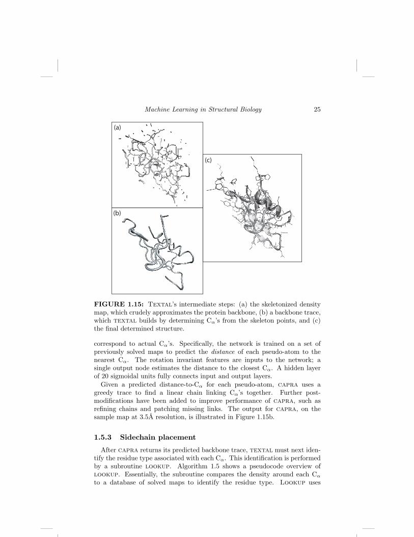
In order to accurately compare maps, capra begins by first normalizingdensity values in the map, ensures feature values from different maps are com-parable. Next, capra skeletonizes the map, creating a trace of pseudo-atomsthat identifies the medial axis of some density map contour. Figure 1.15a il-lustrates this skeletonization. This trace is a very crude approximation of thebackbone, and may traverse the side-chains or form multiple distinct chains.

A feed-forward neural network – a nonlinear function approximator usedfor both classification and regression – is trained to learn which pseudo-atoms


(c)

(a)

(b)

FIGURE 1.15: Textal’s intermediate steps: (a) the skeletonized densitymap, which crudely approximates the protein backbone, (b) a backbone trace,which textal builds by determining Cα’s from the skeleton points, and (c)the final determined structure.

correspond to actual Cα’s. Specifically, the network is trained on a set ofpreviously solved maps to predict the distance of each pseudo-atom to thenearest Cα. The rotation invariant features are inputs to the network; asingle output node estimates the distance to the closest Cα. A hidden layerof 20 sigmoidal units fully connects input and output layers.

Given a predicted distance-to-Cα for each pseudo-atom, capra uses agreedy trace to find a linear chain linking Cα’s together. Further post-modifications have been added to improve performance of capra, such asrefining chains and patching missing links. The output for capra, on thesample map at 3.5A resolution, is illustrated in Figure 1.15b.

1.5.3 Sidechain placement

After capra returns its predicted backbone trace, textal must next iden-tify the residue type associated with each Cα. This identification is performedby a subroutine lookup. Algorithm 1.5 shows a pseudocode overview oflookup. Essentially, the subroutine compares the density around each Cα

to a database of solved maps to identify the residue type. Lookup uses

26

ALGORITHM 1.5: Textal’s lookup subroutine for placingsidechains.Given: electron density map M, backbone trace X = {xi}Find: all-atom protein model

for ~xi ∈ X doF← rotation-invariant features in a neighborhood around xi

N← k examples in DB minimizing weighted Euclidean distancefor ~ni ∈ N do

~n′i ← optimal superposition of ~ni into map at ~xi

scorei ← RSCC(ni,M(~xi)) // see Equation 1.9endChoose n′i maximizing scorei

Add individual atoms of n′i to modelend

textal’s rotation invariant features, and builds a database of feature vec-tors corresponding to Cα’s in solved maps. To determine the residue typeof an unknown region of density, lookup finds the nearest neighbors in thedatabase, using weighted Euclidian distance:

D(ρ1||ρ2) =[ ∑

i

λi ·(Fi(ρ1)− Fi(ρ2)

)2]1/2

(1.16)

Above, Fi refers to the ith feature in the vector, while ρ1 and ρ2 are two regionsof density. Feature weights λi are optimized to maximize similarity betweenmatching regions and minimize between non-matching regions, where groundtruth is the optimally-aligned RSCC (Equation 1.9). Textal sets weightsusing the slider algorithm [20] which considers features pairwise to determinea good set of weights.

Since information is lost when representing a region as a rotation invariantfeature vector, the nearest neighbor in the database does not always corre-spond to the best-matching region. Therefore, lookup keeps the top k regions– those with the lowest Euclidean distance – and considers these for a moretime-consuming RSCC computation (see Equation 1.9). Ideally, lookupwants to find the rotation and translation of each of the k regions to maxi-mize this correlation coefficient. It quickly approximates this optimal rotationand translation by aligning the moments of inertia between the template den-sity region ρ1 and target density region ρ2. Lookup computes the real-spacecorrelation at each alignment, and selects the highest-correlated candidate.Finally, lookup retrieves the translated and rotated coordinated atoms ofthe top-scoring candidate and places them in the model.


1.5.4 Post-processing routines

Since each residue’s atoms are copied from previous examples and gluedtogether in the density map, the model produced by lookup may containsome physically infeasible bond lengths, bond angles, or φ−ψ torsion angles.Textal’s final step is improving the model using a few simple post-processingheuristics. First, lookup often reverses the backbone direction of a residue;textal’s post-processing makes sure that all chains are oriented in a consis-tent direction. Refinement, like that of arp/warp, corrects improper bondlengths and bond angles, iteratively moving individual atoms to fit the densitymap better. Finally, textal takes into account the target protein’s sequenceto fix mismatched residues.

Textal makes use of a provided sequence by aligning the map-determinedmodel sequence to the provided input sequence, using a Smith-Watermandynamic-programming alignment. If there is agreement between the sequencesabove some threshold, then a second lookup pass corrects residues where thealignment disagrees. In this second pass, lookup is restricted to only considerresidues of the type indicated by the sequence alignment. Like resolve,textal’s end result is a complete all-atom protein model, illustrated for ourexample map in Figure 1.15c.

1.5.5 Discussion

Textal – like resolve – uses higher-order constructs than atoms in or-der to successfully solve low-quality maps. In practice, textal works wellon maps at around 3A resolution. Textal’s key contribution is the use ofrotation-invariant features to recognize patterns in the map. This feature rep-resentation allows accurate Cα identification using a neural network; it alsodoes well at classification of amino-acid type. Textal tends to do better thanresolve at sidechain identification due to this feature set. One key shortcom-ing, however, is limiting the initial backbone trace to skeleton points in thedensity map. In very poor maps, skeletonization is inaccurate; this is in partresponsible for textal’s failure in maps worse than 3A. However, textalhas successfully employed previously solved structures and domain knowledgefrom structural biology to produce an accurate map interpretation.

1.6 acmi

Acmi (automatic crystallographic map interpreter) is a recent method de-veloped by DiMaio et al. for tracing protein backbones in poor-quality (3 to4A resolution) density maps [19]. Acmi takes a probabilistic approach to elec-tron density map interpretation, finding the most likely layout of the backbone

28


Construct and match 5-mer templates

Infer locations conditioned on sequence

Choose maximum-marginal locations

a priori probability that AAi is at location x

marginal probability that AAi is at location x

Cα-trace model

FIGURE 1.16: A flowchart of acmi.

under some likelihood function. This likelihood function takes into accountlocal matches to the density map as well as the global pairwise configurationof residues. The key difference between acmi and the preceding methods isthat acmi represents each residue not as a single location, but rather as a com-plete probability distribution over the full electron density map. This property– not forcing each residue to a single location – is advantageous as it naturallyhandles noise in the map, errors in the input sequence, and disordered regionsin the protein.

Figure 1.16 shows a high-level overview of acmi. The algorithm is comprisedof two main components: a local matching component that probabilisticallymatches individual amino acids to the density map, and a global constraintcomponent where the backbone chain is probabilistically refined from the localmatches. Global refinement is based on physical laws governing the structureof proteins. Acmi’s key is an efficient inference algorithm that determines themost probable physically feasible backbone trace in an electron density map.

1.6.1 Local matching

The local matching component of acmi is provided the density map and theprotein’s amino acid sequence. It computes, for each residue in the protein,a probability distribution Pi(~wi) over all locations ~wi in the unit cell. Thisprobability distribution reflects the probability that residue i is at positionand orientation ~wi in the unit cell.

Acmi’s local match – shown in Algorithm 1.6 – is based upon a 5-mer (thatis, a polypeptide sequence five amino-acids in length) search. Using a set ofpreviously solved structures, acmi first constructs a basis set of structures de-scribing the conformational space of each 5-mer in the protein. Acmi searchesfor each of these fragments in the map over all translations and rotations. Thislocal search produces – for each residue i – an estimated probability distrib-ution of that residue i’s location and orientation in the unit cell, Pi(~wi).


ALGORITHM 1.6: Acmi’s local-matching algorithmGiven: sequence seq, electron density map MFind: probability distribution Pi(~wi) of each residue over map

for each residue seqi ∈ seq doN← instances of 5-mer 〈seqi−2 . . . seqi+2〉 from PDBC← cluster N, extract centroidsλi ← cluster weightsfor each cluster centroid cj ∈ C do

t(~wi)← Perform 6D search for cj over density mapUse a tuning set to convert t(~wi) to probabilities Pij(~wi)

end

Pi(~wi)←∑

clusters j

λiPij(~wi)

end

1.6.1.1 Constructing a sequence-specific 5-mer basis set

Given some 5-amino-acid sequence, acmi uses the Protein Data Bank (PDB),a repository of solved protein structures, to find all the instances of this se-quence. If there are fewer than fifty such instances, acmi considers “near-neighbors” (using the PAM-120 score, a measure of amino-acid similarity)until at least fifty distinct conformations are available. It uses these struc-tures to represent the conformational space of the given 5-mer.

Searching for all these conformations in the electron density map is wasteful,because many are redundant, so acmi clusters the structures into a smallernumber of distinct conformations, representing each cluster with a single “cen-tral” instance (or centroid) of that cluster and a numeric weight. Acmi storesnon-centroid instances from each cluster as well for tuning. Clustering usesthe all-atom root mean squared deviation (RMSd) as a distance metric. Acmican perform this clustering process in advance for all 3.2×106 possible 5-mers.

1.6.1.2 Searching for 5-mer centroid fragments

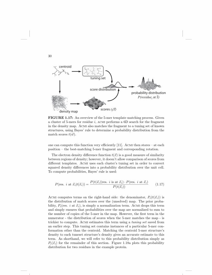
Given a protein sequence, acmi considers the 5-mer sequence centered ateach amino-acid. It extracts the fragments which represent the conforma-tional space of that sequence, which it learns from the clustering process,and searches the density map for these fragments. Figure 1.17 illustrates thisprocess graphically. Given these fragments and a resolution limit, acmi buildsan expected density map for each fragment. Then, at each map location, acmicomputes the standardized mean squared electron density difference t(~x) be-tween the map and the fragment. Notice that this t(~x) is the same densitymap similarity function employed by resolve, shown in Equation 1.7.

Acmi’s fragment search is a 6D search: it considers every rotation of a frag-ment at every location in the map. Using fffear’s FFT-based convolution,

30

centroid

density map

tuning set

scores ti(x)

score distributionprobability distribution

P(residuei at x)

FIGURE 1.17: An overview of the 5-mer template matching process. Givena cluster of 5-mers for residue i, acmi performs a 6D search for the fragmentin the density map. Acmi also matches the fragment to a tuning set of knownstructures, using Bayes’ rule to determine a probability distribution from thematch scores t(~w).

one can compute this function very efficiently [11]. Acmi then stores – at eachposition – the best-matching 5-mer fragment and corresponding rotation.

The electron density difference function t(~x) is a good measure of similaritybetween regions of density; however, it doesn’t allow comparison of scores fromdifferent templates. Acmi uses each cluster’s tuning set in order to convertsquared density differences into a probability distribution over the unit cell.To compute probabilities, Bayes’ rule is used:

P (res. i at ~xi|t(~xi)) =P (t(~xi)|res. i is at ~xi) · P (res. i at ~xi)

P (t(~xi))(1.17)

Acmi computes terms on the right-hand side: the denominator, Pi(t(~xi)) isthe distribution of match scores over the (unsolved) map. The prior proba-bility, Pi(res. i at ~xi), is simply a normalization term. Acmi drops this termand simply ensures that probabilities over the map are normalized to sum tothe number of copies of the 5-mer in the map. However, the first term in thenumerator - the distribution of scores when the 5-mer matches the map - istrickier to compute. Acmi estimates this term using a tuning set saved froman earlier step. This tuning set contains instances of a particular 5-mer con-formation other than the centroid. Matching the centroid 5-mer structure’sdensity to each tuneset structure’s density gives an accurate estimate to thisterm. As shorthand, we will refer to this probability distribution simply asPi(~xi) for the remainder of this section. Figure 1.18a plots this probabilitydistribution for two residues in the example protein.


(a)

(b)

(c)

GLU20 ALA60

GLU20 ALA60

FIGURE 1.18: Intermediate steps in acmi’s structure determination:(a) the matching probability distributions Pi(~xi) on two residues, GLU20 andALA60, contoured at p = 10−4, (b) the marginal probability distributions overthe same two residues, and (c) the final (backbone-only) model, each residueshaded by likelihood (darker is more likely).

1.6.2 Global constraints

Given each residue’s independent probability distribution over the unit cell,Pi(~xi), acmi accounts for global constraints (enforced by physical feasibility)of a conformation by modeling the protein using a pairwise Markov field. Apairwise Markov field defines the joint probability distribution over a set ofvariables as a product of potential functions defined over vertices and edgesin an undirected graph (see Figure 1.19).

1.6.2.1 Markov field model

Formally, the graph G = (V, E) consists of a set of nodes i ∈ V connected byedges (i, j) ∈ E . Each node in the graph is associated with a (hidden) randomvariable ~wi ∈ W, and the graph is conditioned on a set of observation vari-ables M. Each vertex has a corresponding observation potential ψi(~wi,M),and each edge is associated with an edge potential ψij(~wi, ~wj). Then, theprobability of a complete trace W is:

P (W|M) ∝∏

(i,j)∈E

ψij(~wi, ~wj)×∏i∈V

ψi(~wi,M) (1.18)

Probabilistic inference finds the labels W = {~wi} maximizing this probability,given some M.

32

ALA GLY LYS LEU ... ... ALA GLY LYS LEU ... ... ALA GLY LYS LEU ... ...

observational potentials ψi

adjacency potentials ψadj

occupancy potentials ψocc

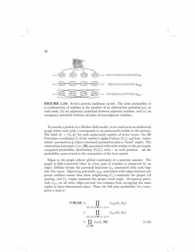
FIGURE 1.19: Acmi’s protein backbone model. The joint probability ofa conformation of residues is the product of an observation potential psii ateach node, (b) an adjacency potential between adjacent residues, and (c) anoccupancy potential between all pairs of non-adjacent residues..

To encode a protein in a Markov field model, acmi constructs an undirectedgraph where each node i corresponds to an amino-acid residue in the protein.The label ~wi = 〈~xi, ~qi〉 for each amino-acid consists of seven terms: the 3DCartesian coordinates ~xi of the residue’s alpha Carbon (Cα), and four “orien-tation” parameters ~qi (three rotational parameters plus a “bend” angle). Theobservation potential ψi(wi,M) associated with each residue is the previouslycomputed probability distribution Pi(~xi), with – at each position – all theprobability mass stored in the orientation of the best match.

Edges in the graph enforce global constraints in a pairwise manner. Thegraph is fully-connected (that is, every pair of residues is connected by anedge); DiMaio breaks the potential functions ψij associated with each edgeinto two types. Adjacency potentials ψadj associated with edges between ad-jacent residues ensure that these neighboring Cα’s maintain the proper 3.8spacing, and Cα triples maintain the proper bend angle. Occupancy poten-tials ψocc on all other edges prevent two residues from occupying the sameregion in three-dimensional space. Thus, the full joint probability of a trace,given a map is:

P (W|M) ∝∏

(~wi, ~wj)∈W,|i−j|=1

ψadj(~wi, ~wj)

×∏

(~wi, ~wj)∈W,|i−j|>1

ψocc(~wi, ~wj)

×∏

~wi∈W

ψi(~wi,M) (1.19)


1.6.2.2 Adjacency potentials

Adjacency potentials, which connect every neighboring pair of residues, arethe product of two constraining functions, a distance constraint function anda rotational constraint function:

ψadj(~wi, ~wj) = px(||~xi − ~xj ||) · pθ(~wi, ~wj) (1.20)

In proteins, the Cα - Cα distance is a nearly invariant 3.8A. Thus, thepotential px takes the form of a tight Gaussian (σ = 0.03A) around this idealvalue, softened a bit for grid effects. Acmi defines the potential pθ using analternate parameterization of the angular parameters ~qi.

Specifically, acmi represents these four degrees of freedom as two pairs ofθ − φ spherical coordinates: the most likely direction of the forward (i + 1)residue and the backward (i−1) residue. When matching the 5-mer templatesinto the density map, at each location xi, acmi stores four values – θb, φb,θf , and φf - indicating the direction of both adjacent Cα in the rotated,best-matching 5-mer.

The angular constraint function pθ is then – in each direction – a fixed-width Gaussian on a sphere, centered on this preferred orientation, (θb, φb) or(θf , φf ).

1.6.2.3 Occupancy potentials

Occupancy potentials ensure that two residues do not occupy the samelocation in space. They are defined independently of orientation, and aremerely a step function that constrains two (nonadjacent) Cα’s be at least3A apart. It is in this structural potential function that acmi deals withcrystallographic symmetry, by ensuring that all crystallographic copies are atleast 3A apart:

ψocc(~wi, ~wj) =

1(

minsymmetric

transforms K||xi −K(xj)||

)≥ 3.0A

0 otherwise(1.21)

Multiple chains in the asymmetric unit are also handled by acmi: edges en-forcing occupancy constraints fully connect separate chains.

1.6.2.4 Tracing the backbone

Acmi’s backbone trace – shown in Algorithm 1.7 – is equivalent to findingthe labels W = {~wi} that maximize the probability of Equation 1.18. Sincethe graph over which the joint probability is defined contains loops, finding anexact solution is infeasible (dynamic programming can solve this in quadratictime for graphs with no loops). Acmi uses belief propagation (BP) to computean approximation to the marginal probability for each residue i (that is, thefull joint probability with all but one variable summed out). Acmi choosesthe label for each residue that maximizes this marginal as the final trace.

34

ALGORITHM 1.7: Acmi’s global-constraint algorithmGiven: individual residue probability distributions Pi(~wi)Find: approximate marginal probabilities bi(~wi)

∀i initialize belief b0i (~wi) to Pi(~wi)repeat

for each residue i dobi(~wi)← Pi(~wi)for each residue j 6= i do

// compute incoming messageif |i− j| = 1 then

mnj→i(~wi)←

∫~wjψadj(~wi, ~wj)× bj

mn−1i→j

(~wj)d~wj

elsemn

j→i(~wi)←∫

~wjψocc(~wi, ~wj)× bj(~wj)d~wj

end

// aggregate messagesbi(~wi)← bi(~wi)×mn

j→i(~wi)end

enduntil (bi’s converge)

Belief propagation is an inference algorithm - based on Pearl’s polytreealgorithm for [21] Bayesian networks - that computes marginal probabilitiesusing a series of local messages. At each iteration, an amino acid computesan estimate of its marginal distribution (i.e., an estimate of the residue’slocation in the unit cell) as the product of that node’s local evidence ψi andall incoming messages:

bni (~wi) ∝ ψi(~wi,M)×∏

j∈Γ(i)

mnj→i(~wi) (1.22)

Above, the belief bni at iteration n is the best estimate of residue i’s marginaldistribution,

bni (~wi) ≈∑~w0

. . .∑~wi−1

∑~wi+1

. . .∑~wN

P (W,M) (1.23)

Message update rules determine each message:

mnj→i(~wi) ∝

∫~wj

ψij(~wi, ~wj)× ψj(~wj ,M)

×∏

k∈Γ(j)\i

mn−1k→j(xj) d~wj (1.24)


Computing the message from j to i uses all the messages going into node jexcept the message from node i. When using BP in graphs with loops, such asacmi’s protein model, there are no guarantees of convergence or correctness;however, empirical results show that loopy BP often produces a good approx-imation to the true marginal [22]. On the example protein, acmi computesthe marginal distributions shown in Figure 1.18b.

To represent belief and messages, acmi uses a Fourier-series probabilitydensity estimate. That is, in the Cartesian coordinates ~xi, marginal distribu-tions are represented as a set of 3-dimensional Fourier coefficients fk, where,given an upper-frequency limit, (H,K,L):

bni (~xi) =H,K,L∑h,k,l=0

fhkl × e−2πi(~xi�〈h,k,l〉) (1.25)

In rotational parameters, acmi divides the unit cell into sections, and in eachsection stores a single orientation ~qi. These orientations correspond to thebest-matching 5-mer orientation. More importantly, these stored orientationsand are not updated by belief propagation: messages are independent of therotational parameters ~qi.

To make this method tractable, acmi approximates all the outgoing occu-pancy messages at a single node:

mnj→i(~wi) ∝

∫~wj

ψocc(~wi, ~wj)×bnj (~wj)d~wj

mn−1i→j (~wj)

(1.26)

The approximation drops the denominator above:

mnj→∗(~wi) ∝

∫~wj

ψocc(~wi, ~wj)× bnj (~wj)d~wj (1.27)

That is, acmi computes occupancy messages using all incoming messages tonode j including the message from node i. All outgoing occupancy messagesfrom node j, then, use the same estimate. Acmi caches the product of alloccupancy messages

∏imi→∗. This reduces the running time of each iteration

in a protein with n amino acids from O(n2) to O(n).Additionally, acmi quickly computes all occupancy messages using FFTs:

F[mn

j→i(~wi)]

= F[ψocc(~wi, ~wj)

]×F

[( ∏mn−1

j→i(~wi))]

(1.28)

This is possible only because the occupancy potential is a function of thedifference of the labels on the connected nodes, ψocc(~wi, ~wj) = f(||~xi − ~xj ||).

Finally, although acmi computes the complete marginal distribution at eachresidue, a crystallographer is only interested in a single trace. The backbonetrace consists of the locations for each residue that maximize the marginal

36

probability:

~w∗i =arg max

~wi

bi(~wi)

= arg max~wi

ψi(~wi,M)×∏

j∈Γ(i)

mnj→i(~wi) (1.29)

Acmi’s backbone trace on the example map is illustrated in Figure 1.18c.The backbone trace is shaded by confidence: since acmi computes a completeprobability distribution, it can return not only a putative trace, but alsoa likelihood associated with each amino acid. This likelihood provides thecrystallographer with information about what areas in the trace are likelyflawed; acmi can also produce a high-likelihood partial trace suitable for phaseimprovement.

1.6.3 Discussion

Acmi’s unique approach to density map interpretation allows for an accu-rate trace in extremely poor maps, including those in the 3 to 4A resolutionrange. Unlike the other residue-based methods, acmi is model-based. That is,it constructs a model based on the protein’s sequence, then searches the mapfor that particular sequence. Acmi then returns the most likely interpreta-tion of the map, given the model. This is in contrast to textal and resolvewhich search for “some backbone” in the map, then align the sequence tothis trace after the fact. This makes acmi especially good at sidechain iden-tification; even in extremely bad maps, acmi correctly identifies a significantportion of residues. Unfortunately, acmi also has several shortcomings. Re-quiring complete probability distributions for the location of each residue isespecially time consuming; this has limited the applicability of the methodso far. Additionally, in poor maps, belief propagation fails to converge to asolution, although in these cases a partial trace is usually obtained. By incor-porating probabilistic reasoning with structural biology domain knowledge,acmi has pushed the limit of interpretable maps even further.

1.7 Conclusion

A key step in determining protein structures is interpreting electron densitymaps. In this area, bioinformatics has played a key role. This chapter de-scribes how four different algorithms have approached the problem of electrondensity map interpretation:

• The warpntrace procedure in arp/warp was the first method devel-oped for automatic density map interpretation. Today, it is still the most


widely used method by crystallographers. Arp/warp uses an “atom-level” technique in which free atoms are first placed into the densitymap, free atoms are next linked into chains introducing constraints, andfinally, the combined model is refined to better explain the map. Themethod iterates through these three phases, at each iteration using thepartial model to improve the map. Because it works at the level ofindividual atoms, it requires 2.3A or better map resolution.

• Resolve is a method that searches for higher-level constructs – aminoacids and secondary structure elements – than arp/warp’s atom-levelmethod. Consequently, it produces accurate traces in poor-quality (around3A) electron density maps, unsolvable by arp/warp. It, too, is widelyused by crystallographers. Resolve begins by matching short secondary-structure fragments to the maps, then uses a large fragment library toextend these matches. Finally, overlapping matches are merged in agreedy fashion, and sidechains are traced. Incorporating structural do-main knowledge is key to this method’s success.

• Textal also accurately interprets medium to low resolution (2 to 3A),using residue-level matching. It represents regions of density as a vectorof rotation-invariant features. This alternate representation serves sev-eral purposes. It is used to learn a classifier to identify Cα’s, and it is alsoused to recognize the residue type of each putative Cα through a data-base comparison. The classifier is also very well suited to identifying theresidue type in a given region, making it more accurate than resolvein this respect. Additionally, textal’s rotation-invariant representa-tion enables fast matching of regions of density. This allows textal toeasily make use of previously solved structures in its map interpretation,providing accurate traces even in poor-quality maps.

• Acmi uses a probabilistic model to trace protein backbones in poor-quality (3 to 4A resolution) density maps. It finds the most likely lay-out of the backbone under a likelihood function which takes into accountlocal matches to the density map as well as the global pairwise configu-ration of residues. Unlike other methods, acmi represents each residuenot as a single location but as a probability distribution over the entiredensity map. Also unlike other approaches, it constructs a model basedon the protein’s sequence, and finds the most likely trace of that par-ticular sequence in the density map. Acmi’s probabilistic, model-basedapproach results in accurate tracing and sidechain identification at poorresolutions.

As each of these methods extended the limit of what resolution maps areautomatically interpreted, they brought with them two things: first, a higher-level “basic construct” at which the algorithm searches, and second, betterincorporation of structural domain knowledge. These two key aspects are

38

what enables interpretation in maps where individual atoms are not distin-guishable, and in the future, what will extend the threshold of interpretationfurther.

As fewer and fewer fine details are visible in poor-resolution maps, algo-rithms must use a higher and higher level basic construct – that is, the tem-plate for which they search – in order to be robust against blurred details.Arp/warp has had success when most atoms are visible in the map. If in-dividual atoms are blurred out, the atom-level method will fail. However, aresidue-based method like textal – which will locate amino acids assumingentire residues are not blurred – is robust enough to handle interpretationwhen atom details are unclear. Similarly, using secondary-structure elementsallows even better interpretation. Probabilistic methods like acmi take thisstill further: its interpretation considers a single flexible protein-sized element,and is robust enough to handle maps where entire residues are indistinguish-able.

Another important feature of these methods is the increasing use of struc-tural domain knowledge. In a way, this makes sense: the crystallographerstask is inherently no different than that of the ab initio protein folding al-gorithm. A crystallographer simply has the assistance of a “picture” of theprotein (the density map). All four methods use structural domain knowl-edge, by employing previous solved structures in model building. Primarily,these structures are used in the construction of a set of “representative frag-ments;” however, acmi and textal also use previously solved structures tolearn model parameters. Future methods will increasingly rely on such domainknowledge.

In the future, with the rising popularity of high-throughput structure de-termination, automated map interpretation methods will play a significantrole. Improvements in laboratory techniques are producing density maps ata faster rate. In addition, experimental techniques such as cryo-electron mi-croscopy are producing density maps that approach 5-6A resolution, and arecontinually improving. Automatically determining structure from maps of thisquality will be increasingly important. To further extend the limit of whatmaps are interpretable, automated interpretation techniques will need to usemore domain knowledge, and consider searching not for a single residue or asingle tripeptide, but rather entire proteins, probabilistically. Providing au-tomated systems with increasing amounts of a crystallographer’s “expertise”is key to future improvements in these methods.

Acknowledgements

This work supported by NLM grant 1R01 LM008796-01 and NLM Grant1T15 LM007359-01. The authors would also like to thank George Phillips andTom Ioerger for assistance in writing this chapter.

References

[1] B. Rost and C. Sander (1993). Prediction of protein secondary structureat better than 70% accuracy. J Mol Biol.

[2] G. Rhodes (2000). Crystallography Made Crystal Clear. Academic Press.

[3] J. Abrahams, R. De Graaff (1998). New developments in phase refine-ment. Curr Opin Struct Biol.

[4] S. Russell and P. Norvig (1995). Artificial Intelligence: A Modern Ap-proach. Prentice Hall.

[5] T. Mitchell (1997). Machine Learning. McGraw-Hill.

[6] V. Lamzin and K. Wilson (1993). Automated refinement of protein mod-els. Acta Cryst.

[7] A. Perrakis, T. Sixma, K. Wilson and V. Lamzin (1997). wARP: Im-provement and extension of crystallographic phases by weighted averag-ing of multiple refined dummy atomic models. Acta Cryst.

[8] R. Morris, A. Perrakis and V. Lamzin (2002). ARP/wARP’s model-building algorithms: the main chain. Acta Cryst.

[9] J. Greer (1974). Three-dimensional pattern recognition. J Mol Biol.

[10] L. Leherte, J. Glasgow, K. Baxter, E. Steeg and S. Fortier (1997). Analy-sis of three-dimensional protein images. JAIR.

[11] K. Cowtan (2001). Fast Fourier feature recognition. Acta Cryst.

[12] T. Oldfield (2001). A number of real-space torsion-angle refinement tech-niques for proteins, nucleic acids, ligands and solvent. Acta Cryst.

[13] T. Terwilliger (2002). Automated main-chain model-building bytemplate-matching and iterative fragment extension. Acta Cryst.

[14] T. Terwilliger (2002). Automated side-chain model-building and se-quence assignment by template-matching. Acta Cryst.

[15] D. Levitt (2001). A new software routine that automates the fitting ofprotein X-ray crystallographic electron density maps. Acta Cryst.

[16] T. Ioerger, T. Holton, J. Christopher and J. Sacchettini (1999). TEX-TAL: A pattern recognition system for interpreting electron densitymaps. Proc ISMB.

0-8493-0052-5/00/$0.00+$.50c© 2001 by CRC Press LLC 39

40 References

[17] T. Ioerger and J. Sacchettini (2002). Automatic modeling of proteinbackbones in electron density maps via prediction of C-alpha coordi-nates. Acta Cryst.

[18] K. Gopal, T. Romo, E. Mckee, K. Childs, L. Kanbi, R. Pai, J. Smith,J. Sacchettini and T. Ioerger (2005). TEXTAL: Automated crystallo-graphic protein structure determination. Proc. IAAI.

[19] F. DiMaio, J. Shavlik and G. Phillips (2006). A probabilistic approachto protein backbone tracing in electron density maps. Proc ISMB.

[20] K. Gopal, T. Romo, J. Sacchettini and T. Ioerger (2004). Weightingfeatures to recognize 3D patterns of electron density in X-ray proteincrystallography. Proc CSB.

[21] J. Pearl (1988). Probabilistic Reasoning in Intelligent Systems. MorganKaufman, San Mateo.

[22] K. Murphy, Y. Weiss, and M. Jordan (1999). Loopy belief propagationfor approximate inference: An empirical study. Proc. UAI.

chapter 1 · 2008-07-29 · protein, one must ﬁnd a very speciﬁc setting of conditions (i.e.,...

Documents