chapra numerical analysis 18th chapter solution
DESCRIPTION
Chapra Numerical 18th chapter solutionsTRANSCRIPT

1
PROPRIETARY MATERIAL. © The McGraw-Hill Companies, Inc. All rights reserved. No part of this Manual
may be displayed, reproduced or distributed in any form or by any means, without the prior written permission of the
publisher, or used beyond the limited distribution to teachers and educators permitted by McGraw-Hill for their
individual course preparation. If you are a student using this Manual, you are using it without permission.
CHAPTER 18
18.1 (a)
991136.0)810(812
90309.00791812.190309.0)10(1
f
%886.0%1001
991136.01
t
(b)
997818.0)910(911
9542425.00413927.19542425.0)10(1
f
%218.0%1001
997818.01
t
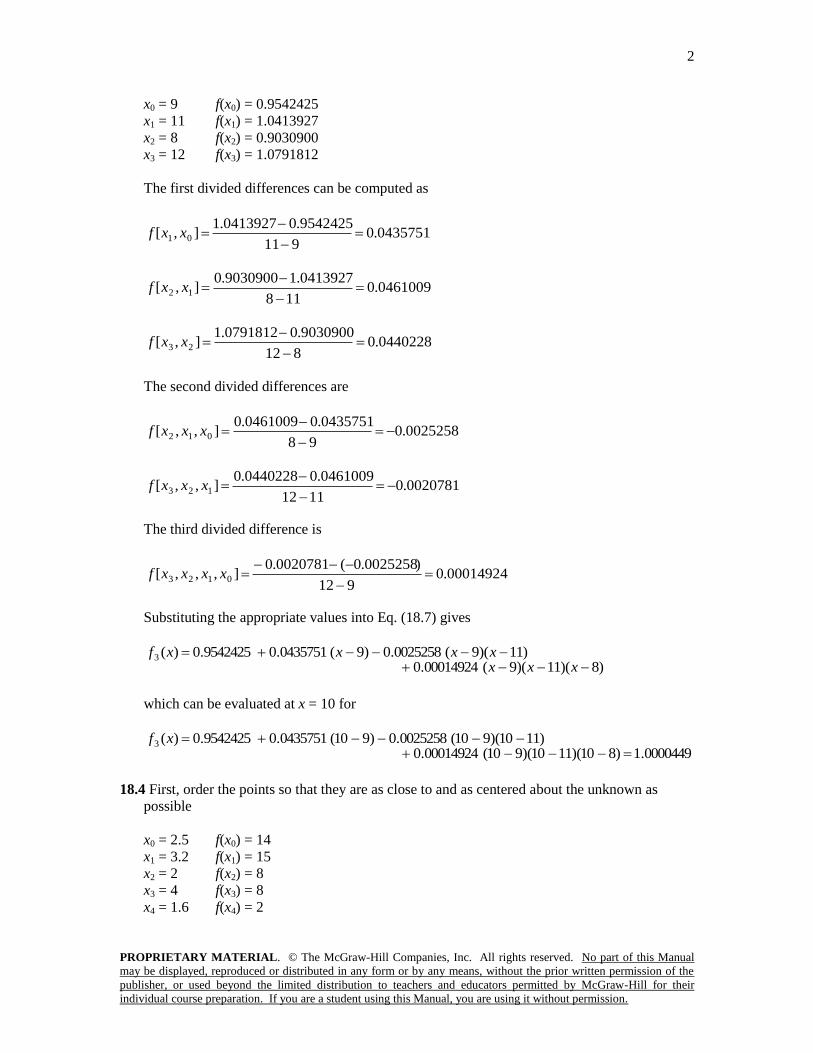
18.2 First, order the points
x0 = 9 f(x0) = 0.9542425
x1 = 11 f(x1) = 1.0413927
x2 = 8 f(x2) = 0.9030900
Applying Eq. (18.4)
b0 = 0.9542425
Equation (18.5) yields
0435751.0911
9542425.00413927.11
b
Equation (18.6) gives
0025258.098
0435751.00461009.0
98
0435751.0118
0413927.19030900.0
2
b
Substituting these values into Eq. (18.3) yields the quadratic formula
)11)(9(0025258.0)9(0435751.09542425.0)(2 xxxxf
which can be evaluated at x = 10 for
0003434.1)1110)(910(0025258.0)910(0435751.09542425.0)10(2 f
18.3 First, order the points
2
PROPRIETARY MATERIAL. © The McGraw-Hill Companies, Inc. All rights reserved. No part of this Manual
may be displayed, reproduced or distributed in any form or by any means, without the prior written permission of the
publisher, or used beyond the limited distribution to teachers and educators permitted by McGraw-Hill for their
individual course preparation. If you are a student using this Manual, you are using it without permission.
x0 = 9 f(x0) = 0.9542425
x1 = 11 f(x1) = 1.0413927
x2 = 8 f(x2) = 0.9030900
x3 = 12 f(x3) = 1.0791812
The first divided differences can be computed as
0435751.0911
9542425.00413927.1],[ 01
xxf
0461009.0118
0413927.19030900.0],[ 12
xxf
0440228.0812
9030900.00791812.1],[ 23
xxf
The second divided differences are
0025258.098
0435751.00461009.0],,[ 012
xxxf
0020781.01112
0461009.00440228.0],,[ 123
xxxf
The third divided difference is
00014924.0912
)0025258.0(0020781.0],,,[ 0123
xxxxf
Substituting the appropriate values into Eq. (18.7) gives
)8)(11)(9(00014924.0 )11)(9(0025258.0)9(0435751.09542425.0)(3
xxxxxxxf
which can be evaluated at x = 10 for
0000449.1)810)(1110)(910(00014924.0 )1110)(910(0025258.0)910(0435751.09542425.0)(3
xf
18.4 First, order the points so that they are as close to and as centered about the unknown as
possible
x0 = 2.5 f(x0) = 14
x1 = 3.2 f(x1) = 15
x2 = 2 f(x2) = 8
x3 = 4 f(x3) = 8
x4 = 1.6 f(x4) = 2

3
PROPRIETARY MATERIAL. © The McGraw-Hill Companies, Inc. All rights reserved. No part of this Manual
may be displayed, reproduced or distributed in any form or by any means, without the prior written permission of the
publisher, or used beyond the limited distribution to teachers and educators permitted by McGraw-Hill for their
individual course preparation. If you are a student using this Manual, you are using it without permission.
Next, the divided differences can be computed and displayed in the format of Fig. 18.5,
i xi f(xi) f[xi+1,xi] f[xi+2,xi+1,xi] f[xi+3,xi+2,xi+1,xi] f[xi+4,xi+3,xi+2,xi+1,xi]
0 2.5 14 1.428571 -8.809524 1.011905 1.847718
1 3.2 15 5.833333 -7.291667 -0.651042
2 2 8 0 -6.25
3 4 8 2.5
4 1.6 2
The first through third-order interpolations can then be implemented as
428571.14)5.28.2(428571.114)8.2(1 f
485714.15)2.38.2)(5.28.2(809524.8)5.28.2(428571.114)8.2(2 f
15.388571.)28.2)(2.38.2)(5.28.2(1.011905 )2.38.2)(5.28.2(809524.8)5.28.2(428571.114)8.2(3
f
The errors estimates for the first and second-order predictions can be computed with Eq.
18.19 as
057143.1428571.14485714.151 R
097143.0485714.15388571.152 R
The error for the third-order prediction can be computed with Eq. 18.18 as
212857.0)48.2)(28.2)(2.38.2)(5.28.2(847718.13 R
18.5 First, order the points so that they are as close to and as centered about the unknown as
possible
x0 = 3 f(x0) = 19
x1 = 5 f(x1) = 99
x2 = 2 f(x2) = 6
x3 = 7 f(x3) = 291
x4 = 1 f(x4) = 3
Next, the divided differences can be computed and displayed in the format of Fig. 18.5,
i xi f(xi) f[xi+1,xi] f[xi+2,xi+1,xi] f[xi+3,xi+2,xi+1,xi] f[xi+4,xi+3,xi+2,xi+1,xi]
0 3 19 40 9 1 0
1 5 99 31 13 1
2 2 6 57 9
3 7 291 48
4 1 3
The first through fourth-order interpolations can then be implemented as
59)34(4019)4(1 f

4
PROPRIETARY MATERIAL. © The McGraw-Hill Companies, Inc. All rights reserved. No part of this Manual
may be displayed, reproduced or distributed in any form or by any means, without the prior written permission of the
publisher, or used beyond the limited distribution to teachers and educators permitted by McGraw-Hill for their
individual course preparation. If you are a student using this Manual, you are using it without permission.
50)54)(34(959)4(2 f
84)24)(54)(34(1 50)4(3 f
48)74)(24)(54)(34(048)4(4 f
Clearly this data was generated with a cubic polynomial since the difference between the 4th
and the 3rd
-order versions is zero.
18.6
18.1 (a):
x0 = 8 f(x0) = 0.9030900
x1 = 12 f(x1) = 1.0791812
991136.00791812.1812
8109030900.0
128
1210)10(1
f
18.1 (b):
x0 = 9 f(x0) = 0.9542425
x1 = 11 f(x1) = 1.0413927
997818.01.0413927911
9109542425.0
119
1110)10(1
f
18.2:
x0 = 8 f(x0) = 0.9030900
x1 = 9 f(x1) = 0.9542425
x2 = 11 f(x2) = 1.0413927
0003434.10413927.1)911)(811(
)910)(810(
9542425.0)119)(89(
)1110)(810(9030900.0
)118)(98(
)1110)(910()10(2
f
18.3:
x0 = 8 f(x0) = 0.9030900
x1 = 9 f(x1) = 0.9542425
x2 = 11 f(x2) = 1.0413927
x3 = 12 f(x3) = 1.0791812
0000449.10791812.1)1112)(912)(812(
)1110)(910)(810(0413927.1
)1211)(911)(811(
)1210)(910)(810(
9542425.0)129)(119)(89(
)1210)(1110)(810(9030900.0
)128)(118)(98(
)1210)(1110)(910()10(3
f
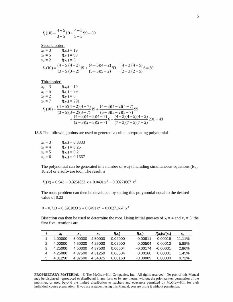
18.7
First order:
x0 = 3 f(x0) = 19
x1 = 5 f(x1) = 99
5
PROPRIETARY MATERIAL. © The McGraw-Hill Companies, Inc. All rights reserved. No part of this Manual
may be displayed, reproduced or distributed in any form or by any means, without the prior written permission of the
publisher, or used beyond the limited distribution to teachers and educators permitted by McGraw-Hill for their
individual course preparation. If you are a student using this Manual, you are using it without permission.
599935
3419
53
54)10(1
f
Second order:
x0 = 3 f(x0) = 19
x1 = 5 f(x1) = 99
x2 = 2 f(x2) = 6
506)52)(32(
)54)(34( 99
)25)(35(
)24)(34(19
)23)(53(
)24)(54()10(2
f
Third order:
x0 = 3 f(x0) = 19
x1 = 5 f(x1) = 99
x2 = 2 f(x2) = 6
x3 = 7 f(x3) = 291
48291)27)(57)(37(
)24)(54)(34(6
)72)(52)(32(
)74)(54)(34(
99)75)(25)(35(
)74)(24)(34(19
)73)(23)(53(
)74)(24)(54()10(3
f
18.8 The following points are used to generate a cubic interpolating polynomial
x0 = 3 f(x0) = 0.3333
x1 = 4 f(x1) = 0.25
x2 = 5 f(x2) = 0.2
x3 = 6 f(x3) = 0.1667
The polynomial can be generated in a number of ways including simultaneous equations (Eq.
18.26) or a software tool. The result is
32
3 00271667.00491.03261833.0943.0)( xxxxf
The roots problem can then be developed by setting this polynomial equal to the desired
value of 0.23
32 00271667.00491.03261833.0713.00 xxx
Bisection can then be used to determine the root. Using initial guesses of xl = 4 and xu = 5, the
first five iterations are
i xl xu xr f(xl) f(xr) f(xl)f(xr) a
1 4.00000 5.00000 4.50000 0.02000 -0.00811 -0.00016 11.11%
2 4.00000 4.50000 4.25000 0.02000 0.00504 0.00010 5.88%
3 4.25000 4.50000 4.37500 0.00504 -0.00174 -0.00001 2.86%
4 4.25000 4.37500 4.31250 0.00504 0.00160 0.00001 1.45%
5 4.31250 4.37500 4.34375 0.00160 -0.00009 0.00000 0.72%
6
PROPRIETARY MATERIAL. © The McGraw-Hill Companies, Inc. All rights reserved. No part of this Manual
may be displayed, reproduced or distributed in any form or by any means, without the prior written permission of the
publisher, or used beyond the limited distribution to teachers and educators permitted by McGraw-Hill for their
individual course preparation. If you are a student using this Manual, you are using it without permission.
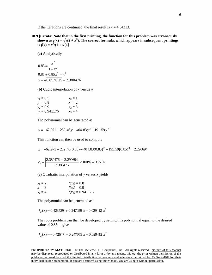
If the iterations are continued, the final result is x = 4.34213.
18.9 [Errata: Note that in the first printing, the function for this problem was erroneously
shown as f(x) = x3/(2 + x
3). The correct formula, which appears in subsequent printings
is f(x) = x2/(1 + x
2).]
(a) Analytically
2
2
185.0
x
x
2285.085.0 xx
380476.215.0/85.0 x
(b) Cubic interpolation of x versus y
y0 = 0.5 x0 = 1
y1 = 0.8 x1 = 2
y2 = 0.9 x2 = 3
y3 = 0.941176 x3 = 4
The polynomial can be generated as
32 59.19183.40446.282971.62 yyyx
This function can then be used to compute
290694.2)85.0(59.191)85.0(83.404)85.0(46.282971.62 32 x
%77.3%100380476.2
290694.2380476.2
t
(c) Quadratic interpolation of y versus x yields
x0 = 2 f(x0) = 0.8
x1 = 3 f(x1) = 0.9
x2 = 4 f(x2) = 0.941176
The polynomial can be generated as
2
2 029412.0247059.0423529.0)( xxxf
The roots problem can then be developed by setting this polynomial equal to the desired
value of 0.85 to give
2
2 029412.0247059.042647.0)( xxxf
7
PROPRIETARY MATERIAL. © The McGraw-Hill Companies, Inc. All rights reserved. No part of this Manual
may be displayed, reproduced or distributed in any form or by any means, without the prior written permission of the
publisher, or used beyond the limited distribution to teachers and educators permitted by McGraw-Hill for their
individual course preparation. If you are a student using this Manual, you are using it without permission.
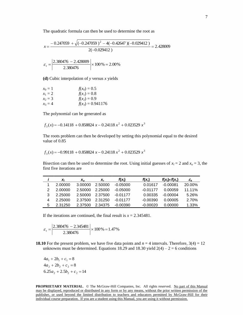
The quadratic formula can then be used to determine the root as
428009.2)029412.0(2
)029412.0)(42647.0(4)247059.0(247059.0 2
x
%00.2%100380476.2
428009.2380476.2
t
(d) Cubic interpolation of y versus x yields
x0 = 1 f(x0) = 0.5
x1 = 2 f(x1) = 0.8
x2 = 3 f(x2) = 0.9
x3 = 4 f(x3) = 0.941176
The polynomial can be generated as
32
3 023529.024118.0858824.014118.0)( xxxxf
The roots problem can then be developed by setting this polynomial equal to the desired
value of 0.85
32
3 023529.024118.0858824.099118.0)( xxxxf
Bisection can then be used to determine the root. Using initial guesses of xl = 2 and xu = 3, the
first five iterations are
i xl xu xr f(xl) f(xr) f(xl)f(xr) a
1 2.00000 3.00000 2.50000 -0.05000 0.01617 -0.00081 20.00%
2 2.00000 2.50000 2.25000 -0.05000 -0.01177 0.00059 11.11%
3 2.25000 2.50000 2.37500 -0.01177 0.00335 -0.00004 5.26%
4 2.25000 2.37500 2.31250 -0.01177 -0.00390 0.00005 2.70%
5 2.31250 2.37500 2.34375 -0.00390 -0.00020 0.00000 1.33%
If the iterations are continued, the final result is x = 2.345481.
%47.1%100380476.2
2.345481380476.2
t
18.10 For the present problem, we have five data points and n = 4 intervals. Therefore, 3(4) = 12
unknowns must be determined. Equations 18.29 and 18.30 yield 2(4) – 2 = 6 conditions
824 111 cba
824 222 cba
145.225.6 222 cba

8
PROPRIETARY MATERIAL. © The McGraw-Hill Companies, Inc. All rights reserved. No part of this Manual
may be displayed, reproduced or distributed in any form or by any means, without the prior written permission of the
publisher, or used beyond the limited distribution to teachers and educators permitted by McGraw-Hill for their
individual course preparation. If you are a student using this Manual, you are using it without permission.
145.225.6 333 cba
152.324.10 333 cba
152.324.10 444 cba
Passing the first and last functions through the initial and final values adds 2 more
26.156.2 111 cba
8416 444 cba
Continuity of derivatives creates an additional 4 – 1 = 3.
2211 44 baba
3322 55 baba
4433 4.64.6 baba
Finally, Eq. 18.34 specifies that a1 = 0. Thus, the problem reduces to solving 11 simultaneous
equations for 11 unknown coefficients,
00082
1515141488
014.6014.600000000015015000000000140114160000000000000000016.112.324.100000000000012.324.100000000015.225.60000000000015.225.6000000001240000000000012
4
4
4
3
3
3
2
2
2
1
1
c
b
a
c
b
a
c
b
a
c
b
which can be solved for
b1 = 15 c1 = 22
a2 = 6 b2 = 39 c2 = 46
a3 = 10.816327 b3 = 63.081633 c3 = 76.102041
a4 = 3.258929 b4 = 14.714286 c4 = 1.285714
The predictions can be made as
64107.13285714.1)4.3(714286.14)4.3(258929.3)4.3( 2 f
76.1046)2.2(39)2.2(6)2.2( 2 f
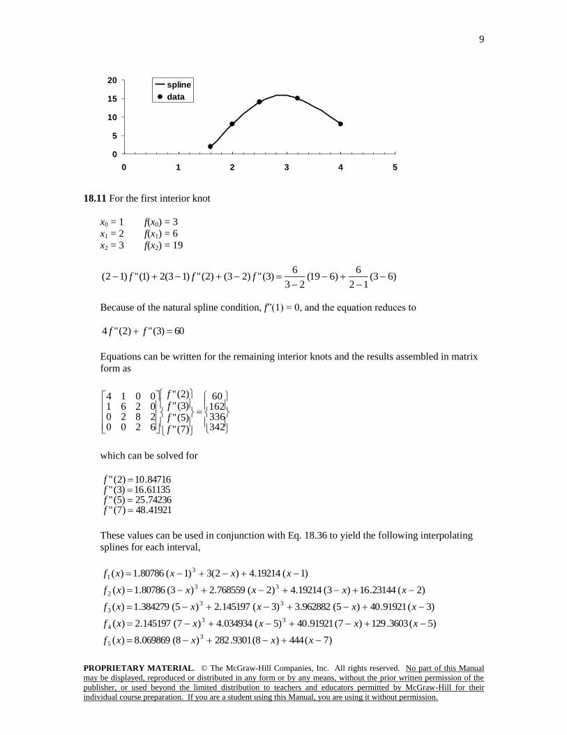
Finally, here is a plot of the data along with the quadratic spline,
9
PROPRIETARY MATERIAL. © The McGraw-Hill Companies, Inc. All rights reserved. No part of this Manual
may be displayed, reproduced or distributed in any form or by any means, without the prior written permission of the
publisher, or used beyond the limited distribution to teachers and educators permitted by McGraw-Hill for their
individual course preparation. If you are a student using this Manual, you are using it without permission.
0
5
10
15
20
0 1 2 3 4 5
spline
data
18.11 For the first interior knot
x0 = 1 f(x0) = 3
x1 = 2 f(x1) = 6
x2 = 3 f(x2) = 19
)63(12
6)619(
23
6)3(")23()2(")13(2)1(")12(
fff
Because of the natural spline condition, f”(1) = 0, and the equation reduces to
60)3(")2("4 ff
Equations can be written for the remaining interior knots and the results assembled in matrix
form as
34233616260
)7("
)5("
)3("
)2("
6200282002610014
f
f
f
f
which can be solved for
41921.48)7("74236.25)5("61135.16)3("84716.10)2("
ffff
These values can be used in conjunction with Eq. 18.36 to yield the following interpolating
splines for each interval,
)1(19214.4)2(3)1(80786.1)( 31 xxxxf
)2(23144.16)3(19214.4)2(768559.2)3(80786.1)( 332 xxxxxf
)3(91921.40)5(962882.3)3(145197.2)5(384279.1)( 333 xxxxxf
)5(3603.129)7(91921.40)5(034934.4)7(145197.2)( 334 xxxxxf
)7(444)8(9301.282)8(069869.8)( 35 xxxxf

10
PROPRIETARY MATERIAL. © The McGraw-Hill Companies, Inc. All rights reserved. No part of this Manual
may be displayed, reproduced or distributed in any form or by any means, without the prior written permission of the
publisher, or used beyond the limited distribution to teachers and educators permitted by McGraw-Hill for their
individual course preparation. If you are a student using this Manual, you are using it without permission.
The interpolating splines can be used to make predictions along the interval. The results are
shown in the following plot.
0
100
200
300
400
500
0 2 4 6 8
(a) The interpolating equations can be used to determine
f3(4) = 48.41157
f2(2.5) = 10.78384
(b)
19)23(23144.16)33(19214.4)23(768559.2)33(80786.1)3( 332 f
19)33(91921.40)35(962882.3)33(145197.2)35(384279.1)3( 333 f
18.12 The points to be fit are
x0 = 3.2 f(x0) = 15
x1 = 4 f(x1) = 8
x2 = 4.5 f(x2) = 2
Using Eq. 18.26 the following simultaneous equations can be generated
1524.102.3 210 aaa
8164 210 aaa
225.205.4 210 aaa
These can be solved for a0 = 11, a1 = 9.25, and a2 = –2.5. Therefore, the interpolating
polynomial is
f(x) = 11 + 9.25x – 2.5x2
18.13 The points to be fit are
x0 = 1 f(x0) = 3
x1 = 2 f(x1) = 6
x2 = 3 f(x2) = 19
x3 = 5 f(x3) = 99

11
PROPRIETARY MATERIAL. © The McGraw-Hill Companies, Inc. All rights reserved. No part of this Manual
may be displayed, reproduced or distributed in any form or by any means, without the prior written permission of the
publisher, or used beyond the limited distribution to teachers and educators permitted by McGraw-Hill for their
individual course preparation. If you are a student using this Manual, you are using it without permission.
Using Eq. 18.26 the following simultaneous equations can be generated
33210 aaaa
6842 3210 aaaa
192793 3210 aaaa
99125255 3210 aaaa
These can be solved for a0 = 4, a1 = –1, a2 = –1, and a3 = 1. Therefore, the interpolating
polynomial is
f(x) = 4 – x – x2 + x
3
18.14 Here is a VBA/Excel program to implement Newton interpolation.
Option Explicit
Sub Newt()
Dim n As Integer, i As Integer
Dim yint(10) As Double, x(10) As Double, y(10) As Double
Dim ea(10) As Double, xi As Double
Sheets("Sheet1").Select
Range("a5").Select
n = ActiveCell.Row
Selection.End(xlDown).Select
n = ActiveCell.Row - n
Range("a5").Select
For i = 0 To n
x(i) = ActiveCell.Value
ActiveCell.Offset(0, 1).Select
y(i) = ActiveCell.Value
ActiveCell.Offset(1, -1).Select
Next i
Range("e3").Select
xi = ActiveCell.Value
Call Newtint(x, y, n, xi, yint, ea)
Range("d5:f25").ClearContents
Range("d5").Select
For i = 0 To n
ActiveCell.Value = i
ActiveCell.Offset(0, 1).Select
ActiveCell.Value = yint(i)
ActiveCell.Offset(0, 1).Select
ActiveCell.Value = ea(i)
ActiveCell.Offset(1, -2).Select
Next i
Range("a5").Select
End Sub
Sub Newtint(x, y, n, xi, yint, ea)
Dim i As Integer, j As Integer, order As Integer
Dim fdd(10, 10) As Double, xterm As Double
Dim yint2 As Double
For i = 0 To n
fdd(i, 0) = y(i)
Next i
For j = 1 To n
12
PROPRIETARY MATERIAL. © The McGraw-Hill Companies, Inc. All rights reserved. No part of this Manual
may be displayed, reproduced or distributed in any form or by any means, without the prior written permission of the
publisher, or used beyond the limited distribution to teachers and educators permitted by McGraw-Hill for their
individual course preparation. If you are a student using this Manual, you are using it without permission.
For i = 0 To n - j
fdd(i, j) = (fdd(i + 1, j - 1) - fdd(i, j - 1)) / (x(i + j) - x(i))
Next i
Next j
xterm = 1#
yint(0) = fdd(0, 0)
For order = 1 To n
xterm = xterm * (xi - x(order - 1))
yint2 = yint(order - 1) + fdd(0, order) * xterm
ea(order - 1) = yint2 - yint(order - 1)
yint(order) = yint2
Next order
End Sub
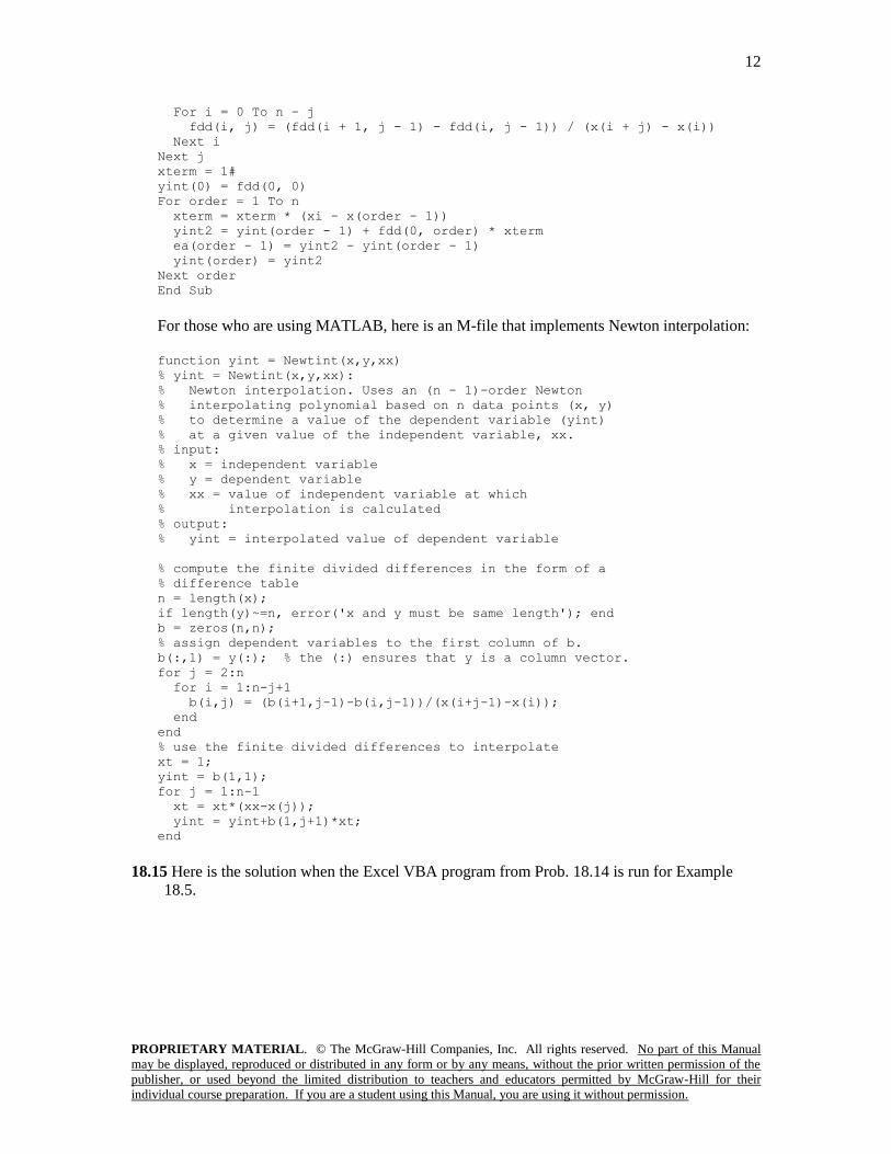
For those who are using MATLAB, here is an M-file that implements Newton interpolation:
function yint = Newtint(x,y,xx)
% yint = Newtint(x,y,xx):
% Newton interpolation. Uses an (n - 1)-order Newton
% interpolating polynomial based on n data points (x, y)
% to determine a value of the dependent variable (yint)
% at a given value of the independent variable, xx.
% input:
% x = independent variable
% y = dependent variable
% xx = value of independent variable at which
% interpolation is calculated
% output:
% yint = interpolated value of dependent variable
% compute the finite divided differences in the form of a
% difference table
n = length(x);
if length(y)~=n, error('x and y must be same length'); end
b = zeros(n,n);
% assign dependent variables to the first column of b.
b(:,1) = y(:); % the (:) ensures that y is a column vector.
for j = 2:n
for i = 1:n-j+1
b(i,j) = (b(i+1,j-1)-b(i,j-1))/(x(i+j-1)-x(i));
end
end
% use the finite divided differences to interpolate
xt = 1;
yint = b(1,1);
for j = 1:n-1
xt = xt*(xx-x(j));
yint = yint+b(1,j+1)*xt;
end
18.15 Here is the solution when the Excel VBA program from Prob. 18.14 is run for Example
18.5.

13
PROPRIETARY MATERIAL. © The McGraw-Hill Companies, Inc. All rights reserved. No part of this Manual
may be displayed, reproduced or distributed in any form or by any means, without the prior written permission of the
publisher, or used beyond the limited distribution to teachers and educators permitted by McGraw-Hill for their
individual course preparation. If you are a student using this Manual, you are using it without permission.
18.16 Here are the solutions when the program from Prob. 18.14 is run for Probs. 18.1 through
18.3.
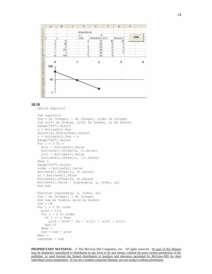
18.17 A plot of the error can easily be added to the Excel application. Note that we plot the
absolute value of the error on a logarithmic scale. The following shows the solution for Prob.
18.4:
The following shows the solution for Prob. 18.5:
14
PROPRIETARY MATERIAL. © The McGraw-Hill Companies, Inc. All rights reserved. No part of this Manual
may be displayed, reproduced or distributed in any form or by any means, without the prior written permission of the
publisher, or used beyond the limited distribution to teachers and educators permitted by McGraw-Hill for their
individual course preparation. If you are a student using this Manual, you are using it without permission.
18.18 Option Explicit
Sub LagrInt()
Dim n As Integer, i As Integer, order As Integer
Dim x(10) As Double, y(10) As Double, xi As Double
Range("a5").Select
n = ActiveCell.Row
Selection.End(xlDown).Select
n = ActiveCell.Row - n
Range("a5").Select
For i = 0 To n
x(i) = ActiveCell.Value
ActiveCell.Offset(0, 1).Select
y(i) = ActiveCell.Value
ActiveCell.Offset(1, -1).Select
Next i
Range("e3").Select
order = ActiveCell.Value
ActiveCell.Offset(1, 0).Select
xi = ActiveCell.Value
ActiveCell.Offset(2, 0).Select
ActiveCell.Value = Lagrange(x, y, order, xi)
End Sub
Function Lagrange(x, y, order, xi)
Dim i As Integer, j As Integer
Dim sum As Double, prod As Double
sum = 0#
For i = 0 To order
prod = y(i)
For j = 0 To order
If i <> j Then
prod = prod * (xi - x(j)) / (x(i) - x(j))
End If
Next j
sum = sum + prod
Next i
Lagrange = sum
15
PROPRIETARY MATERIAL. © The McGraw-Hill Companies, Inc. All rights reserved. No part of this Manual
may be displayed, reproduced or distributed in any form or by any means, without the prior written permission of the
publisher, or used beyond the limited distribution to teachers and educators permitted by McGraw-Hill for their
individual course preparation. If you are a student using this Manual, you are using it without permission.
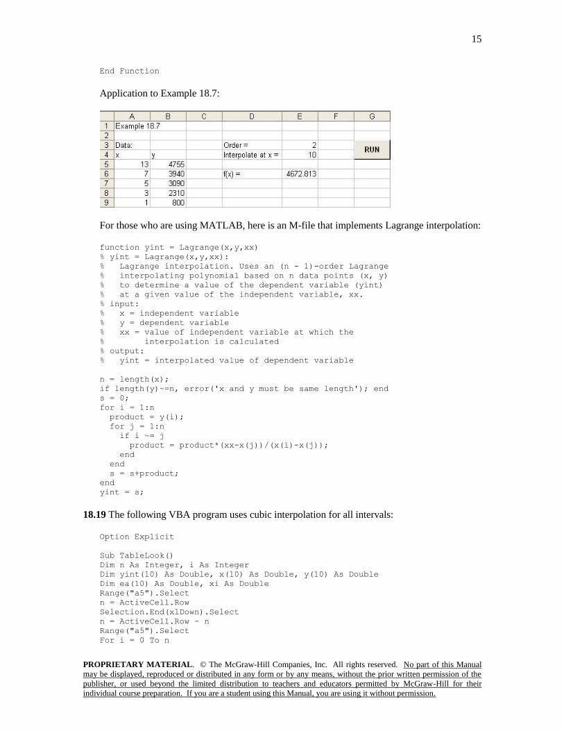
End Function
Application to Example 18.7:
For those who are using MATLAB, here is an M-file that implements Lagrange interpolation:
function yint = Lagrange(x,y,xx)
% yint = Lagrange(x,y,xx):
% Lagrange interpolation. Uses an (n - 1)-order Lagrange
% interpolating polynomial based on n data points (x, y)
% to determine a value of the dependent variable (yint)
% at a given value of the independent variable, xx.
% input:
% x = independent variable
% y = dependent variable
% xx = value of independent variable at which the
% interpolation is calculated
% output:
% yint = interpolated value of dependent variable
n = length(x);
if length(y)~=n, error('x and y must be same length'); end
s = 0;
for i = 1:n
product = y(i);
for j = 1:n
if i ~= j
product = product*(xx-x(j))/(x(i)-x(j));
end
end
s = s+product;
end
yint = s;
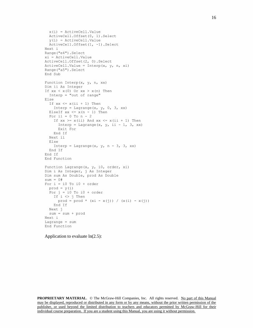
18.19 The following VBA program uses cubic interpolation for all intervals:
Option Explicit
Sub TableLook()
Dim n As Integer, i As Integer
Dim yint(10) As Double, x(10) As Double, y(10) As Double
Dim ea(10) As Double, xi As Double
Range("a5").Select
n = ActiveCell.Row
Selection.End(xlDown).Select
n = ActiveCell.Row - n
Range("a5").Select
For i = 0 To n
16
PROPRIETARY MATERIAL. © The McGraw-Hill Companies, Inc. All rights reserved. No part of this Manual
may be displayed, reproduced or distributed in any form or by any means, without the prior written permission of the
publisher, or used beyond the limited distribution to teachers and educators permitted by McGraw-Hill for their
individual course preparation. If you are a student using this Manual, you are using it without permission.
x(i) = ActiveCell.Value
ActiveCell.Offset(0, 1).Select
y(i) = ActiveCell.Value
ActiveCell.Offset(1, -1).Select
Next i
Range("e4").Select
xi = ActiveCell.Value
ActiveCell.Offset(2, 0).Select
ActiveCell.Value = Interp(x, y, n, xi)
Range("a5").Select
End Sub
Function Interp(x, y, n, xx)
Dim ii As Integer
If xx < x(0) Or xx > x(n) Then
Interp = "out of range"
Else
If xx <= x(ii + 1) Then
Interp = Lagrange(x, y, 0, 3, xx)
ElseIf xx <= x(n - 1) Then
For ii = 0 To n - 2
If xx >= x(ii) And xx <= x(ii + 1) Then
Interp = Lagrange(x, y, ii - 1, 3, xx)
Exit For
End If
Next ii
Else
Interp = Lagrange(x, y, n - 3, 3, xx)
End If
End If
End Function
Function Lagrange(x, y, i0, order, xi)
Dim i As Integer, j As Integer
Dim sum As Double, prod As Double
sum = 0#
For i = i0 To i0 + order
prod = y(i)
For j = i0 To i0 + order
If i <> j Then
prod = prod * (xi - x(j)) / (x(i) - x(j))
End If
Next j
sum = sum + prod
Next i
Lagrange = sum
End Function
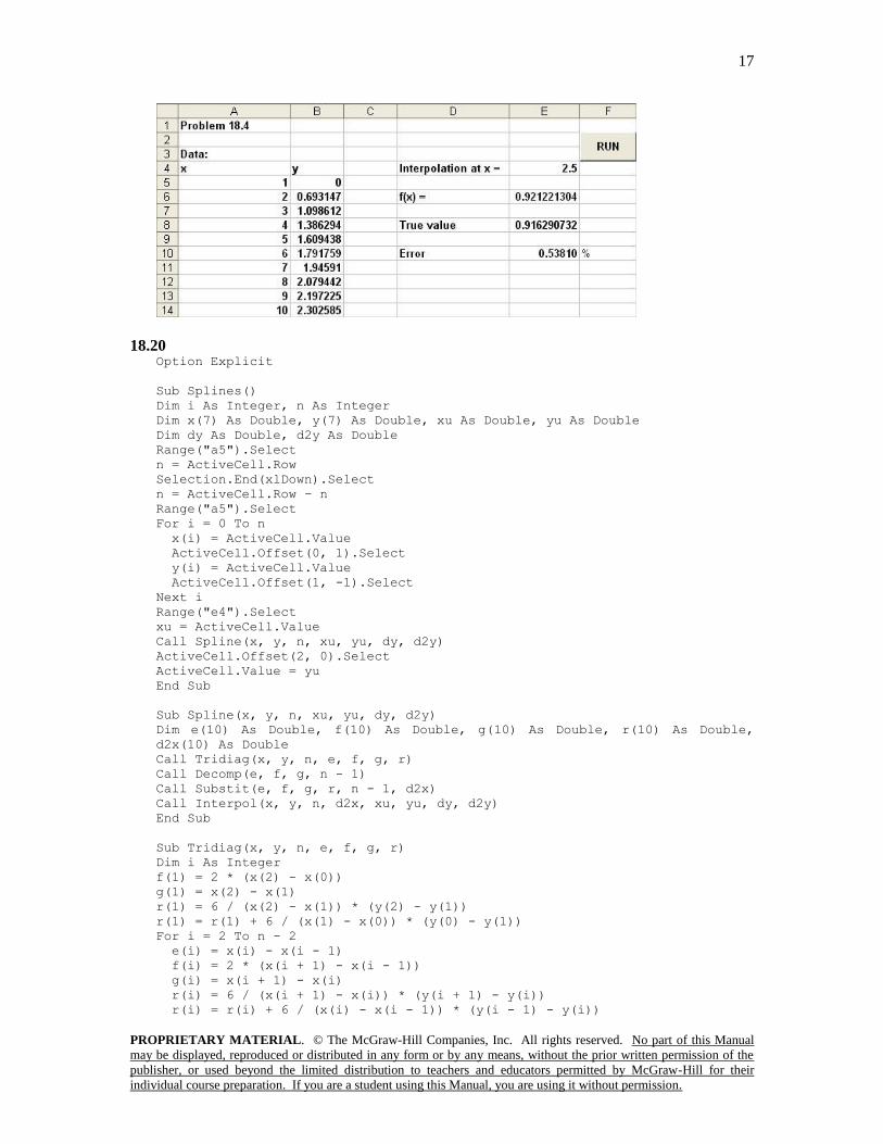
Application to evaluate ln(2.5):
17
PROPRIETARY MATERIAL. © The McGraw-Hill Companies, Inc. All rights reserved. No part of this Manual
may be displayed, reproduced or distributed in any form or by any means, without the prior written permission of the
publisher, or used beyond the limited distribution to teachers and educators permitted by McGraw-Hill for their
individual course preparation. If you are a student using this Manual, you are using it without permission.
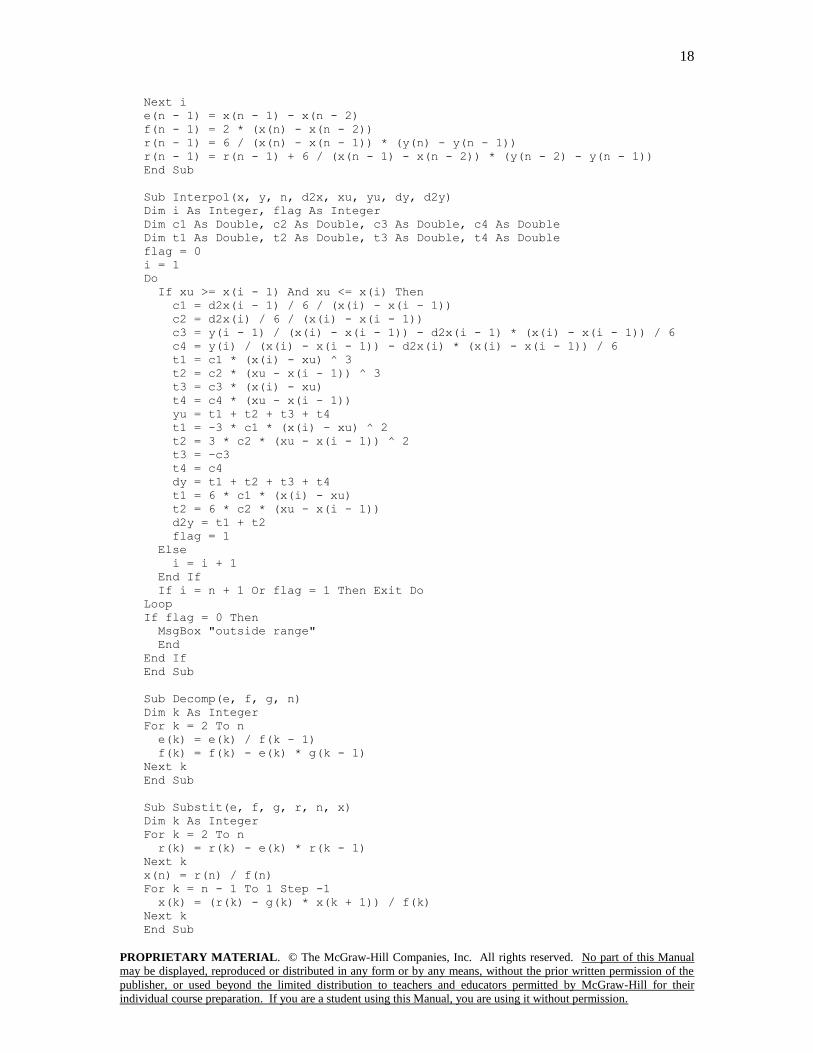
18.20 Option Explicit
Sub Splines()
Dim i As Integer, n As Integer
Dim x(7) As Double, y(7) As Double, xu As Double, yu As Double
Dim dy As Double, d2y As Double
Range("a5").Select
n = ActiveCell.Row
Selection.End(xlDown).Select
n = ActiveCell.Row - n
Range("a5").Select
For i = 0 To n
x(i) = ActiveCell.Value
ActiveCell.Offset(0, 1).Select
y(i) = ActiveCell.Value
ActiveCell.Offset(1, -1).Select
Next i
Range("e4").Select
xu = ActiveCell.Value
Call Spline(x, y, n, xu, yu, dy, d2y)
ActiveCell.Offset(2, 0).Select
ActiveCell.Value = yu
End Sub
Sub Spline(x, y, n, xu, yu, dy, d2y)
Dim e(10) As Double, f(10) As Double, g(10) As Double, r(10) As Double,
d2x(10) As Double
Call Tridiag(x, y, n, e, f, g, r)
Call Decomp(e, f, g, n - 1)
Call Substit(e, f, g, r, n - 1, d2x)
Call Interpol(x, y, n, d2x, xu, yu, dy, d2y)
End Sub
Sub Tridiag(x, y, n, e, f, g, r)
Dim i As Integer
f(1) = 2 * (x(2) - x(0))
g(1) = x(2) - x(1)
r(1) = 6 / (x(2) - x(1)) * (y(2) - y(1))
r(1) = r(1) + 6 / (x(1) - x(0)) * (y(0) - y(1))
For i = 2 To n - 2
e(i) = x(i) - x(i - 1)
f(i) = 2 * (x(i + 1) - x(i - 1))
g(i) = x(i + 1) - x(i)
r(i) = 6 / (x(i + 1) - x(i)) * (y(i + 1) - y(i))
r(i) = r(i) + 6 / (x(i) - x(i - 1)) * (y(i - 1) - y(i))
18
PROPRIETARY MATERIAL. © The McGraw-Hill Companies, Inc. All rights reserved. No part of this Manual
may be displayed, reproduced or distributed in any form or by any means, without the prior written permission of the
publisher, or used beyond the limited distribution to teachers and educators permitted by McGraw-Hill for their
individual course preparation. If you are a student using this Manual, you are using it without permission.
Next i
e(n - 1) = x(n - 1) - x(n - 2)
f(n - 1) = 2 * (x(n) - x(n - 2))
r(n - 1) = 6 / (x(n) - x(n - 1)) * (y(n) - y(n - 1))
r(n - 1) = r(n - 1) + 6 / (x(n - 1) - x(n - 2)) * (y(n - 2) - y(n - 1))
End Sub
Sub Interpol(x, y, n, d2x, xu, yu, dy, d2y)
Dim i As Integer, flag As Integer
Dim c1 As Double, c2 As Double, c3 As Double, c4 As Double
Dim t1 As Double, t2 As Double, t3 As Double, t4 As Double
flag = 0
i = 1
Do
If xu >= x(i - 1) And xu <= x(i) Then
c1 = d2x(i - 1) / 6 / (x(i) - x(i - 1))
c2 = d2x(i) / 6 / (x(i) - x(i - 1))
c3 = y(i - 1) / (x(i) - x(i - 1)) - d2x(i - 1) * (x(i) - x(i - 1)) / 6
c4 = y(i) / (x(i) - x(i - 1)) - d2x(i) * (x(i) - x(i - 1)) / 6
t1 = c1 * (x(i) - xu) ^ 3
t2 = c2 * (xu - x(i - 1)) ^ 3
t3 = c3 * (x(i) - xu)
t4 = c4 * (xu - x(i - 1))
yu = t1 + t2 + t3 + t4
t1 = -3 * c1 * (x(i) - xu) ^ 2
t2 = 3 * c2 * (xu - x(i - 1)) ^ 2
t3 = -c3
t4 = c4
dy = t1 + t2 + t3 + t4
t1 = 6 * c1 * (x(i) - xu)
t2 = 6 * c2 * (xu - x(i - 1))
d2y = t1 + t2
flag = 1
Else
i = i + 1
End If
If i = n + 1 Or flag = 1 Then Exit Do
Loop
If flag = 0 Then
MsgBox "outside range"
End
End If
End Sub
Sub Decomp(e, f, g, n)
Dim k As Integer
For k = 2 To n
e(k) = e(k) / f(k - 1)
f(k) = f(k) - e(k) * g(k - 1)
Next k
End Sub
Sub Substit(e, f, g, r, n, x)
Dim k As Integer
For k = 2 To n
r(k) = r(k) - e(k) * r(k - 1)
Next k
x(n) = r(n) / f(n)
For k = n - 1 To 1 Step -1
x(k) = (r(k) - g(k) * x(k + 1)) / f(k)
Next k
End Sub
19
PROPRIETARY MATERIAL. © The McGraw-Hill Companies, Inc. All rights reserved. No part of this Manual
may be displayed, reproduced or distributed in any form or by any means, without the prior written permission of the
publisher, or used beyond the limited distribution to teachers and educators permitted by McGraw-Hill for their
individual course preparation. If you are a student using this Manual, you are using it without permission.
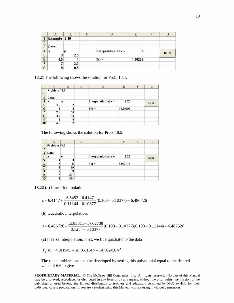
18.21 The following shows the solution for Prob. 18.4:
The following shows the solution for Prob. 18.5:
18.22 (a) Linear interpolation:
486726.6)10377.0108.0(10377.011144.0
4147.65453.64147.6
s
(b) Quadratic interpolation:
487526.6)11144.0108.0)(10377.0108.0(10377.01254.0
02738.1783811.15486726.6
s
(c) Inverse interpolation. First, we fit a quadratic to the data
2
2 982456.54860154.28011945.4)( vvvf
The roots problem can then be developed by setting this polynomial equal to the desired
value of 6.6 to give
20
PROPRIETARY MATERIAL. © The McGraw-Hill Companies, Inc. All rights reserved. No part of this Manual
may be displayed, reproduced or distributed in any form or by any means, without the prior written permission of the
publisher, or used beyond the limited distribution to teachers and educators permitted by McGraw-Hill for their
individual course preparation. If you are a student using this Manual, you are using it without permission.
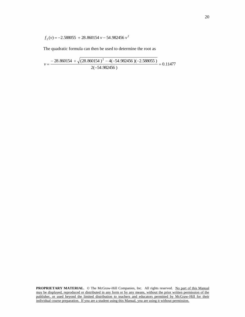
2
2 982456.54860154.28588055.2)( vvvf
The quadratic formula can then be used to determine the root as
11477.0)982456.54(2
)588055.2)(982456.54(4)860154.28(860154.28 2
v