chaotic time series forecasting with …...chaotic time series forecasting with residual analysis...

CHAOTIC TIME SERIES FORECASTINGWITH RESIDUAL ANALYSIS USING

SYNERGY OF ENSEMBLE NEURAL NETWORKS ANDTAGUCHI’S DESIGN OF EXPERIMENTS

BY

MUHAMMAD ARDALANI-FARSAMaster of Applied Science, Mechanical Engineering, Ryerson University, 2006

A dissertationpresented to Ryerson University

in partial fulfillment of therequirements for the degree of

Doctor of Philosophyin the program of

Mechanical Engineering

Toronto, Ontario, Canada, 2010Muhammad Ardalani-Farsa 2010 ©

ii

AUTHOR’S DECLARATION

I hereby declare that I am the sole author of this dissertation

I authorize Ryerson University to lend this dissertation to other institutions or individuals for the

purpose of scholarly research.

I further authorize Ryerson University to reproduce this dissertation by photocopying or by other

means, in total or in part, at the request of other institutions or individuals for the purpose of

scholarly research.

iii

BORROWER’S PAGE

Ryerson University requires the signatures of all persons using or photocopying this dissertation.

Please sign below and give the address and date.

iv

ABSTRACT

Chaotic Time Series Forecasting with Residual Analysis Using Synergy of

Ensemble Neural Networks and Taguchi’s Design of Experiments

Doctor of Philosophy, 2010, Muhammad Ardalani-Farsa, Mechanical Engineering

School of Graduate Studies, Ryerson University

This dissertation aims to develop an effective and practical method to forecast chaotic

time series. Chaotic behaviour has been observed in the areas of marketing, stock

markets, supply chain management, foreign exchange rates, weather forecasting and

many others. An effective forecasting method can reduce the potential risks and

uncertainty and facilitate planning and decision making in chaotic systems.

In this study, residual analysis using a combination of the embedding theorem and

ensemble artificial neural networks is adopted to forecast chaotic time series. Based

on the embedding theorem, the embedding parameters are determined and the time

series is reconstructed into proper phase space points. The embedded phase space

points are fed into the first neural network and trained. The weights and biases are

kept to predict the future values of phase space points and accordingly to obtain

future values of chaotic time series. The residual of the predicted time series is further

analyzed; and, if a chaotic behaviour is observed, then the residuals are processed as a

new chaotic time series and predicted. This iterative residual analysis can be repeated

several times depending on the desired accuracy level and computational efficiency.

Finally, the last neural network is trained using neural networks’ result values of the

time series and the residuals as input and the original time series as output. The initial

weights and biases of the neural networks are improved using genetic algorithms.

Taguchi’s design of experiments is adopted to identify appropriate factor-level

combinations to improve the result of the proposed forecasting method. A systematic

approach is proposed to improve the combination of ensemble artificial neural

networks and their parameters. The proposed methodology is applied to a number of

benchmark and some real life chaotic time series. In addition, the proposed

forecasting method has been applied to financial sector time series, namely, stock

markets and foreign exchange rates. The experimental results confirm that the

proposed method can predict the chaotic time series more effectively in terms of error

indices when compared with other existing forecasting methods in the literature.

v

ACKNOWLEDGEMENTS

I am very thankful to my supervisor, Dr. Saeed Zolfaghari, whose guidance, support and

encouragement from the initial to the final level allowed me to develop this dissertation. I owe

my deepest gratitude to my parents who encouraged me to start my PhD and unconditionally

supported me. It is an honour for me to thank the Director of Mechanical Engineering Graduate

Program, Dr. Greg Kawall, for his abundant support. I am grateful to Dr. Kamran Behdinan for

helping me to smoothly begin my PhD program. Further, I wish to thank the external examiner

of my committee, Dr. Uday Venkatadri, committee chair, Dr. Ana Pejovic-Milic, and other

members of the committee, Dr. Alireza Sadeghian, Dr. Liping Fang and Dr. Mohamad Jaber for

their constructive comments and suggestions. I would like to offer my gratitude to all of those

who have inspired and supported me in any respect during the completion of the dissertation.

Lastly, I would like to thank Dr. Robert Roseberry for reviewing and proofreading my

dissertation.

vi

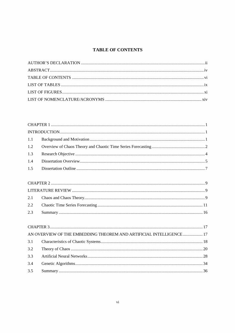
TABLE OF CONTENTS

AUTHOR’S DECLARATION ................................................................................................................ii

ABSTRACT........................................................................................................................................... iv

TABLE OF CONTENTS .......................................................................................................................vi

LIST OF TABLES ................................................................................................................................. ix

LIST OF FIGURES................................................................................................................................ xi

LIST OF NOMENCLATURE/ACRONYMS ....................................................................................... xiv

CHAPTER 1 ........................................................................................................................................... 1

INTRODUCTION................................................................................................................................... 1

1.1 Background and Motivation ........................................................................................................ 1

1.2 Overview of Chaos Theory and Chaotic Time Series Forecasting ................................................ 2

1.3 Research Objective ..................................................................................................................... 4

1.4 Dissertation Overview................................................................................................................. 5

1.5 Dissertation Outline .................................................................................................................... 7

CHAPTER 2 ........................................................................................................................................... 9

LITERATURE REVIEW ........................................................................................................................ 9

2.1 Chaos and Chaos Theory............................................................................................................. 9

2.2 Chaotic Time Series Forecasting ............................................................................................... 11

2.3 Summary .................................................................................................................................. 16

CHAPTER 3.......................................................................................................................................... 17

AN OVERVIEW OF THE EMBEDDING THEOREM AND ARTIFICIAL INTELLIGENCE.................. 17

3.1 Characteristics of Chaotic Systems............................................................................................ 18

3.2 Theory of Chaos ....................................................................................................................... 20

3.3 Artificial Neural Networks........................................................................................................ 28

3.4 Genetic Algorithms................................................................................................................... 34

3.5 Summary .................................................................................................................................. 36

vii

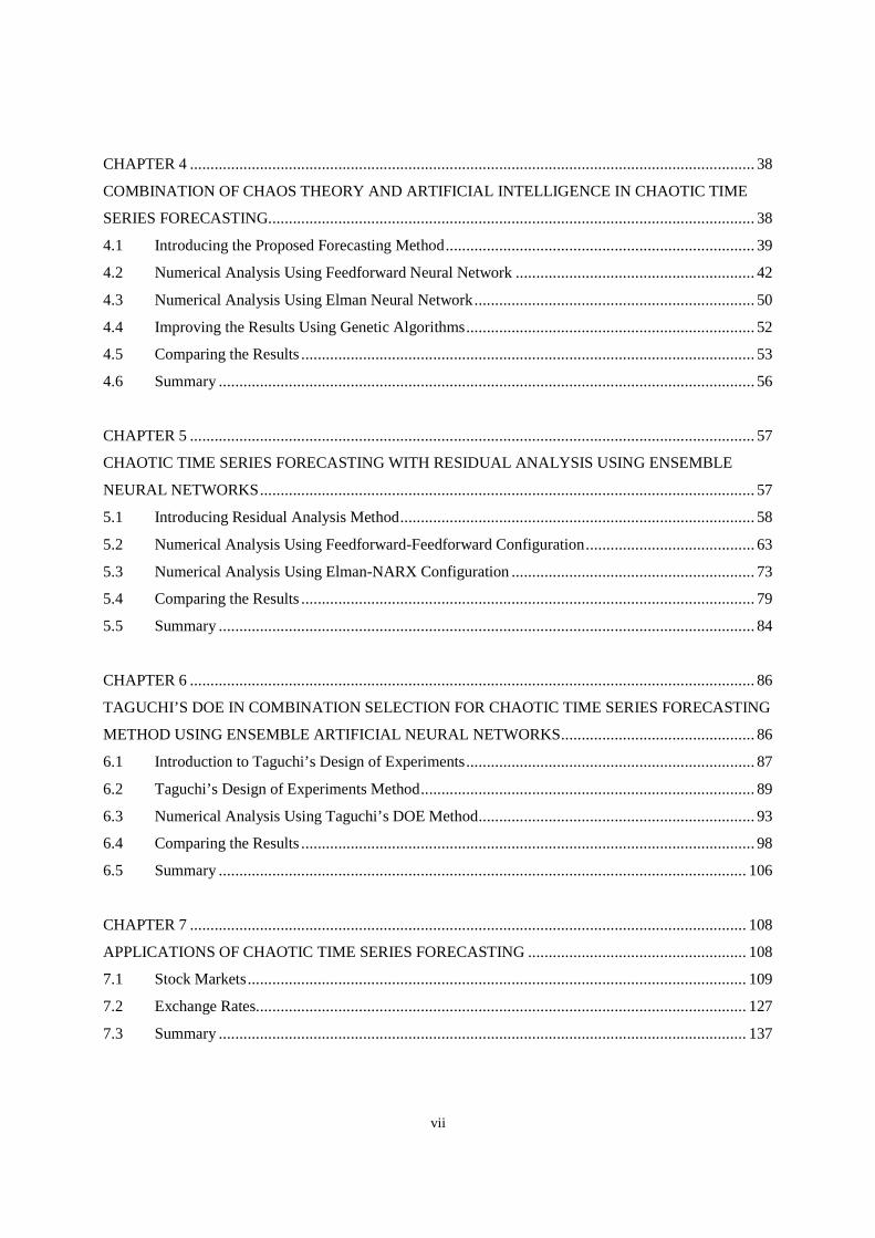
CHAPTER 4 ......................................................................................................................................... 38

COMBINATION OF CHAOS THEORY AND ARTIFICIAL INTELLIGENCE IN CHAOTIC TIME

SERIES FORECASTING...................................................................................................................... 38

4.1 Introducing the Proposed Forecasting Method........................................................................... 39

4.2 Numerical Analysis Using Feedforward Neural Network .......................................................... 42

4.3 Numerical Analysis Using Elman Neural Network.................................................................... 50

4.4 Improving the Results Using Genetic Algorithms...................................................................... 52

4.5 Comparing the Results .............................................................................................................. 53

4.6 Summary .................................................................................................................................. 56

CHAPTER 5 ......................................................................................................................................... 57

CHAOTIC TIME SERIES FORECASTING WITH RESIDUAL ANALYSIS USING ENSEMBLE

NEURAL NETWORKS........................................................................................................................ 57

5.1 Introducing Residual Analysis Method...................................................................................... 58

5.2 Numerical Analysis Using Feedforward-Feedforward Configuration......................................... 63

5.3 Numerical Analysis Using Elman-NARX Configuration ........................................................... 73


5.5 Summary .................................................................................................................................. 84

CHAPTER 6 ......................................................................................................................................... 86

TAGUCHI’S DOE IN COMBINATION SELECTION FOR CHAOTIC TIME SERIES FORECASTING

METHOD USING ENSEMBLE ARTIFICIAL NEURAL NETWORKS............................................... 86

6.1 Introduction to Taguchi’s Design of Experiments...................................................................... 87

6.2 Taguchi’s Design of Experiments Method................................................................................. 89

6.3 Numerical Analysis Using Taguchi’s DOE Method................................................................... 93


6.5 Summary ................................................................................................................................ 106

CHAPTER 7 ....................................................................................................................................... 108

APPLICATIONS OF CHAOTIC TIME SERIES FORECASTING ..................................................... 108

7.1 Stock Markets......................................................................................................................... 109

7.2 Exchange Rates....................................................................................................................... 127

7.3 Summary ................................................................................................................................ 137

viii

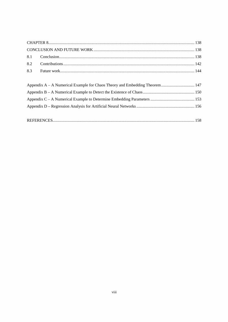
CHAPTER 8........................................................................................................................................ 138

CONCLUSION AND FUTURE WORK .............................................................................................. 138

8.1 Conclusion.............................................................................................................................. 138

8.2 Contributions .......................................................................................................................... 142

8.3 Future work............................................................................................................................. 144

Appendix A – A Numerical Example for Chaos Theory and Embedding Theorem............................... 147

Appendix B – A Numerical Example to Detect the Existence of Chaos ................................................ 150

Appendix C – A Numerical Example to Determine Embedding Parameters ......................................... 153

Appendix D – Regression Analysis for Artificial Neural Networks ...................................................... 156

REFERENCES.................................................................................................................................... 158

ix

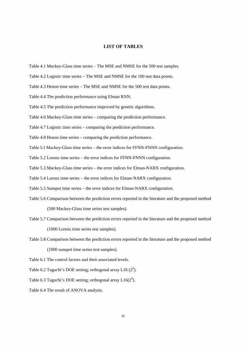
LIST OF TABLES

Table 4.1 Mackey-Glass time series – The MSE and NMSE for the 500 test samples.

Table 4.2 Logistic time series – The MSE and NMSE for the 100 test data points.

Table 4.3 Henon time series – The MSE and NMSE for the 500 test data points.

Table 4.4 The prediction performance using Elman RNN.

Table 4.5 The prediction performance improved by genetic algorithms.

Table 4.6 Mackey-Glass time series – comparing the prediction performance.

Table 4.7 Logistic time series – comparing the prediction performance.

Table 4.8 Henon time series – comparing the prediction performance.

Table 5.1 Mackey-Glass time series – the error indices for FFNN-FNNN configuration.

Table 5.2 Lorenz time series – the error indices for FFNN-FNNN configuration.

Table 5.3 Mackey-Glass time series – the error indices for Elman-NARX configuration.

Table 5.4 Lorenz time series – the error indices for Elman-NARX configuration.

Table 5.5 Sunspot time series – the error indices for Elman-NARX configuration.

Table 5.6 Comparison between the prediction errors reported in the literature and the proposed method

(500 Mackey-Glass time series test samples).


(1000 Lorenz time series test samples).


(1000 sunspot time series test samples).

Table 6.1 The control factors and their associated levels.

Table 6.2 Taguchi’s DOE setting; orthogonal array L16 (28).

Table 6.3 Taguchi’s DOE setting; orthogonal array L16(28).

Table 6.4 The result of ANOVA analysis.

x

Table 6.5 The response table for Lorenz time series, Mackey-Glass time series, sunspot time series and far-

infrared NH3 laser time series.


(1000 Lorenz time series validation data).


(500 Mackey-Glass time series validation data).


(1000 sunspot time series validation data).


(100 far-infrared NH3 laser time series validation data).


(94 British Airlines stock test data).


(82 Southwest Airlines stock test data).


(70 Ryanair stock test data).


(500 Lucent stock test data).


(157 EUR/USD test data).


(500 USD/JPY test data).

Table D.1 The regression analysis between the proposed Elman and feedforward neural network response

and the corresponding targets when applied to Mackey-Glass, Logistic and Henon time series.

xi

LIST OF FIGURES

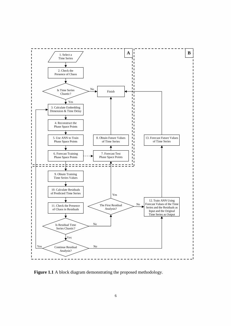
Figure 1.1 A block diagram demonstrating the proposed methodology.

Figure 3.1 Single node in a feedforward neural network.

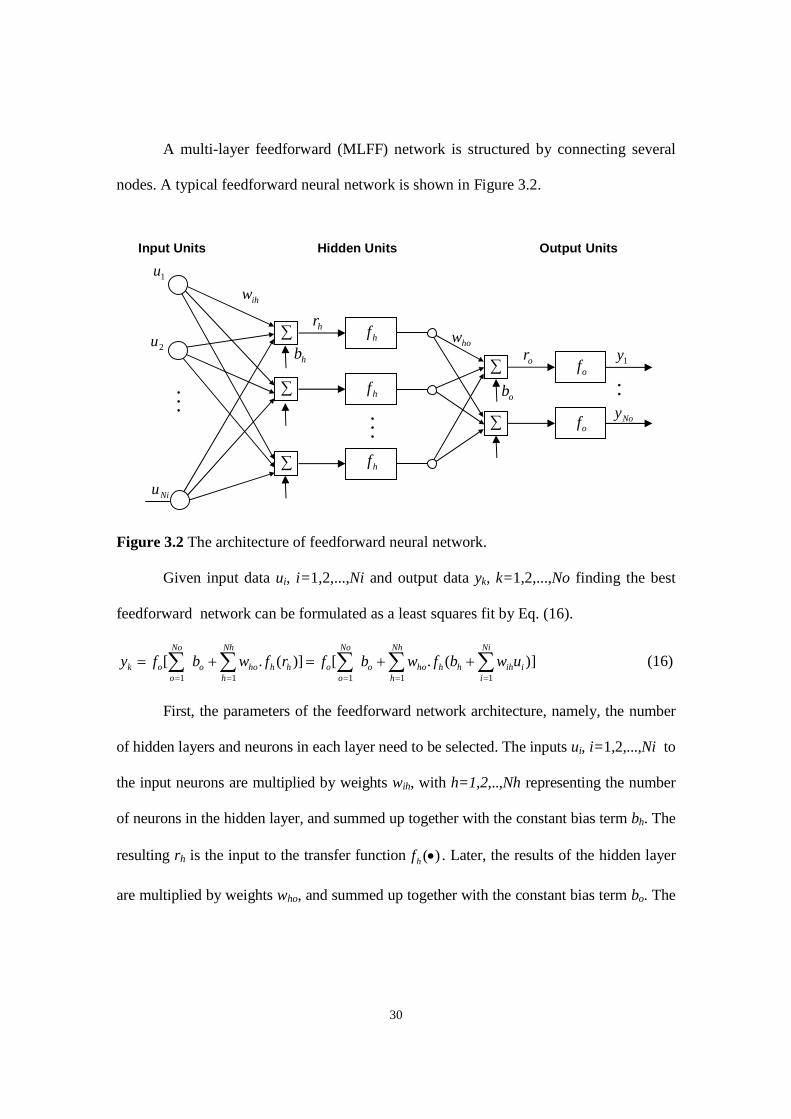
Figure 3.2 The architecture of feedforward neural network.

Figure 3.3 The architecture of Elman recurrent neural network.

Figure 3.4 The architecture of NARX neural network.

Figure 3.5 A string representing gene and chromosome in genetic algorithms.

Figure 3.6 Schematic illustration of genetic algorithms.

Figure 4.1 A block diagram demonstrating the proposed forecasting method.

Figure 4.2 Mackey-Glass chaotic time series a) in time domain, b) in phase space domain.

Figure 4.3 Comparison of Mackey-Glass time series and forecast values using FFNN.

Figure 4.4 Logistic chaotic time series a) in time domain, b) in phase space domain.

Figure 4.5 Comparison of Logistic time series data and forecast values using FFNN.

Figure 4.6 Henon chaotic time series a) in time domain, b) in phase space domain.

Figure 4.7 Comparison of Henon time series data and forecast values using FFNN.

Figure 4.8 Comparison of M-G time series data and forecast values using Elman ANN.

Figure 4.9 Comparison of Logistic time series data and forecast values using Elman RNN.

Figure 4.10 Comparison of Henon time series data and forecast values using Elman RNN.

Figure 5.1 A FFNN correlating the original and residual time series prediction to original time series.

Figure 5.2 A NARX network correlating the original and residuals forecasts to original time series.

Figure 5.3 A FFNN correlating the original time series prediction and the prediction of residuals in various

levels to original time series.

Figure 5.4 Mackey-Glass Time Series – Comparing the original time series data and the predicted values.

Figure 5.5 Mackey-Glass time series –First residual values a) in the time domain b) in the phase space domain.

Figure 5.6 Mackey-Glass time series – The comparison of the first residual values and the predicted values.

xii

Figure 5.7 Mackey-Glass time series – The second residual values, a)in time domain b) in phase space domain.

Figure 5.8 Mackey-Glass time series – The comparison of the second residual values and the predicted values.

Figure 5.9 The comparison between original Mackey-Glass time series and the final predicted values.

Figure 5.10 Lorenz time series, a) in time domain, b) in phase space domain.

Figure 5.11 Lorenz time series – The comparison of the original time series samples and the predicted

values based on feedforward network.

Figure 5.12 Lorenz time series – The first residuals a) in time domain, b) in phase space domain.

Figure 5.13 Lorenz time series – the comparison of the first residual and predicted values.

Figure 5.14 The comparison between original Lorenz time series and the final predicted values.

Figure 5.15 Sunspot time series – The comparison of the original time series samples and the predicted

values based on Elman network.

Figure 5.16 The comparison between original sunspot time series and the final predicted values.


Figure 6.2 Comparison between original Mackey-Glass time series and the final predicted values.

Figure 6.3 The comparison between original sunspot time series and the final predicted values.

Figure 6.4 The marked area in Figure 6.3.

Figure 6.5 Comparison between original far-infrared NH3 laser series and final forecast values.

Figure 7.1 The daily closing price of British Airlines stock for Jan. 1, 2003 to Jan. 10, 2005.

Figure 7.2 Largest Lyapunov exponent graph for British Airlines stock data.

Figure 7.3 British Airlines stock data in phase space domain.

Figure 7.4 British Airlines stock data – Comparing the original stock data and the predicted values.

Figure 7.5 British Airlines stock data – The comparison of the first residual values and the predicted values.

Figure 7.6 British Airlines stock data – The comparison of the second residual values and the predicted values.

Figure 7.7 The comparison between original British Airlines stock data and the final predicted values.

Figure 7.8 The daily closing price of Southwest Airlines stock December 18, 2002 to November 17, 2004.

xiii

Figure 7.9 The comparison between original Southwest Airlines stock data and the final predicted values.

Figure 7.10 The daily closing price of Ryanair stock for the period May 06, 2003 to March 17, 2005.

Figure 7.11 The comparison between original Ryanair stock data and the final predicted values.

Figure 7.12 The scaled daily closing price of Lucent incorporated stock for the period November 28, 1998

to November 28, 2003.

Figure 7.13 The comparison between scaled Lucent stock data and the final predicted values.

Figure 7.14 The exchange rate EUR/USD from February 01, 2002 to October 31, 2008.

Figure 7.15 Largest Lyapunov exponent graph for EUR/USD data.

Figure 7.16 The comparison between original EUR/USD data time series and the final predicted values.

Figure 7.17 The daily exchange rates between the US dollar and the Japanese yen for the period January

01, 2003 and December 31, 2006.

Figure 7.18 USD/JPY data in the phase space domain with D = 3 and T = 5.

Figure 7.19 USD/JPY data – Comparing the original test data and the predicted values.

Figure 7.20 USD/JPY data – The comparison of the first residual values and the predicted values.

Figure 7.21 The comparison between original USD/JPY data and the final predicted values.

Figure A.1 The original states of Lorenz system.

Figure A.2 Lorenz time series reconstructed into the phase space points with T = 3 and D = 3.

Figure B.1 Henon chaotic time series with 1000 data points.

Figure B.2 Power spectrum plot for Henon time series.

Figure B.3 Largest Lyapunov exponent plot for Henon time series.

Figure C.1 Average mutual information graph for Henon time series.

Figure C.2 Cao’s graph to identify embedding dimension for Henon time series.

Figure C.3 Henon time series in phase space domain.

Figure D.1 The regression analysis between the feedforward network response and the corresponding

targets when applied to Mackey-Glass time series.

xiv

LIST OF NOMENCLATURE/ACRONYMS

Rn : vector space

n : dimension of vector space Rn

s(t) : state of the original chaotic system

Q : function governing a chaotic system

x(t) : observe quantity

Y(t) : phase space points

D : embedding dimension

T : time delay

)(kX : Fourier transform

)(kP : power spectrum

: Lyapunov exponent

H : Hurst exponent

C(r) : mean of points in a sphere of radius r

dc : correlation dimension

)(TI : average mutual information

Pr(x(t), x(t+T)) : joint probability density at time t and t+T leading to x(t) and x(t+T)

Pr(x(t)) : probability densities at time t resulting to x(t)

Pr(x(t+T)) : probability densities at time t+T resulting to x(t+T)

NN : nearest neighbour

E(D) : Cao’s embedding dimension parameter

E1(D) : ratio of E(D+1) over E(D)

uj : ANN’s input to the input layer

wjk : ANN’s weight

xv

k : number of neurons in the hidden layer

bk : ANN’s bias

rk : input to the transfer function f

f : ANN’s transfer function

yk : ANN’s output

Ni : number of neurons in input layer

No : number of neurons in output layer

Nh : number of neurons in hidden layer

)(hf : hidden layer transfer function

)(of : output layer transfer function

bo : output layer bias

bh : hidden layer bias

who : hidden layer weight

wih : output layer weight

ud : NARX network’s input delay

yd : NARX network’s output delay.

hiw1 : weights of the connections between the first input units and the hidden units

hiw 2 : weights of the connections between the second input units and the hidden units

tp : probability of selecting the chromosomes for mating

ft : fitness of the chromosome

G : estimation of function Q

iy

: predicted data

y : average of observed data

1D : the first residual time series embedding dimension

xvi

1T : the first residual time series time delay,

)(1 te : the first residual value

x'(i) : prediction value of the time series

)(1 ie : prediction value of the first residual time series

)(2 te : the second residual value

)(2 ie : prediction value of the second residual time series

M : level of residual analysis

S/N : signal-to-noise ratio

Purelin : linear transfer function

tansig : hyperbolic tangent sigmoid transfer function

traingdx : gradient descent with momentum and adaptive learning rate backpropagation

trainbr : Bayesian regulation backpropagation

trainlm : Levenberg-Marquardt backpropagation

largelyap : function to calculate the largest Lyapunov exponent

takens_estimator : function to calculate correlation dimension

amutual : function to calculate time delay

cao : function to calculate embedding dimension

xvii

AFS : Adaptive Fuzzy System

AI : Artificial intelligence

AMB : Adaptive Memory-Based regression

ANFIS : Adaptive-Network-based Fuzzy Interface System

ANN : Artificial Neural Network

ANOVA : Analysis of Variance

AR : Autoregressive

ARMA : Autoregressive Moving Average

ARX : Autoregressive model with eXogenous input

ATNN : Backpropagation continuous-time FFNN with Adaptable Time delays

BGALR : Breeder Genetic Algorithms with Line Recombination

BPNN : Backpropagation continuous-time FFNN with fixed time delays

CCPND : Complete Counter-Propagation Networks with Delays

CHF/USD : Exchange rates between the Swiss franc and the US dollar

CPN : Counter-Propagation Networks

DCS-LMM : Dynamic Cell Structures combined with Local Linear Models

DECS : Dynamic Evolving Computation System

DEM/FRF : Exchange rates between the Deutsche mark and the French franc

DLE : Distributed Local Experts

DLM : Distributed Local Models

DOE : Design of Experiments

EP : Error Propagation

EPNet : Evolvable Programming Net

ESN : Echo-State Networks

EUR/GBP : Exchange rates between the Euro and the Britain pound

EUR/USD : Exchange rates between the Euro and the US dollar

xviii

FD : Fractal Dimension

FFNN : Feedforward Neural Network

FIR : Finite Impulse Response neural network

FNT : Flexible Neural Tree

GA : Genetic Algorithms

GDP : Gross Domestic Product

GFPE : Genetic Fuzzy Predictor Ensemble

GMDH-GA : Group Method of Data Handling using Genetic Algorithms

GP : Gaussian Process

GPM : Genetic Programming-based Modeling

HMM : Hidden Markov Model

LLE : Largest Lyapunov Exponent

LoLiMoT : Locally Linear neuro-fuzzy Model with locally linear model Tree

LSTM : Long Short-Term Memory

MANFIS : Multi-input multi-output Adaptive-Network-based Fuzzy Interface System

MAPE : Mean Absolute Percentage Error

MLP : Multi-Layer Perceptron neural network

MSE : Mean Squared Error

MS-SVR : Multi-Scale Support Vector Regression

NARX : Nonlinear Autoregressive model with eXogenous input

NMSE : Normalized Mean Squared Error

OA : Orthogonal Arrays

OLS : Ordinary least squares

PANN : Polynomial Artificial Neural Networks

PNN : Probabilistic Neural Networks

PRESS : Predicted Sum of Squares

xix

RBF : Radial Basis Function network

RL-GP : Recurrent Linear – Genetic Programming

RMSE : Root Mean Squared Error

RNN : Recurrent Neural Network

RSOM : Recurrent Self-Organizing Map

SOM : Self-Organizing Map

SVM : Support Vector Machine

SVR : Support Vector Regression

TAR : Threshold Autoregression

TDNN : Time Delay Neural Network

USD/JPY : Exchange rates between the US dollar and the Japanese yen

Volterra-TLS : Volterra Total Least Square

VQIT : Vector-Quantization using Information Theoretic

WNN : Wavelet Neural Networks

1

CHAPTER 1

INTRODUCTION

1.1 Background and Motivation

Over the last several decades, prediction of chaotic time series has been a popular and

challenging subject. Chaos theory as a new area of mathematics has been used to analyze

chaotic systems and draw the hidden information from random-look data produced by

chaotic systems. Chaotic time series are deterministic systems and inherit a high degree of

complexity. Although chaotic time series show the characteristics of dynamical systems as

random, in the embedding phase space, they present deterministic behaviour [1].

The application of chaos theory is becoming increasingly widespread in a variety

of disciplines. An early application of chaos theory was proposed in modelling and data

analysis of mixing processes [2,3]. Chaos theory has been applied to the control of robot

servos where the robot can learn from its environment and recognize the beginning of

random behaviour [4]. Chaos has also been applied in communications, the optimization

of telephone exchanges [5] and the transmission of digital signals [6]. Data analysis

methods developed for the analysis of chaotic behaviour have been applied to bulk

chemical reactions [7].

Prediction of nonlinear time series is a useful method to evaluate characteristics of

dynamical systems. Prediction of chaotic time series has been observed in the areas of

marketing system [8,9], foreign exchange rates [10], signal processing [11], supply chain

2

management [12], traffic flow [13], power load [14], weather forecasting [15], sunspot

[16], cardiovascular control [17] and many others. Due to the importance of these fields

and widespread applications of chaotic systems in real life, the interest in a robust

technique to predict chaotic time series has increased.

There are several types of time series such as periodic, seasonal, stochastic, chaotic

and others. To differentiate between deterministic and stochastic data, it is necessary to

search for similar or nearby states and compare their progress over time. Determining the

difference between the time progress of the nearby states, the random data can be

differentiated from deterministic data. For deterministic data the error will remain either

small for stable data or evolve exponentially with time for chaotic data. The error for

stochastic data will be randomly distributed [18]. In this study, the focus is to identify a

chaotic time series from non-chaotic data and forecast the future of the chaotic time series.

Many of the proposed forecasting methods in the literature are either ineffective

when applied to chaotic time series or difficult to implement. The motivation of this

dissertation is to develop a more easy-to-use, effective in terms of error indices and

practical method to forecast chaotic time series.

1.2 Overview of Chaos Theory and Chaotic Time Series Forecasting

Chaos theory, as an essential part of nonlinear theory, has provided an appropriate

tool to study the characteristics of the dynamical systems and predict the trend of

complex systems. There are four fundamental characteristics for chaotic systems:

aperiodic, that is, the same state will not be repeated; bounded, meaning that

neighbouring states remain within a finite range and do not approach infinity;

3

deterministic, meaning that there is a governing rule with no random term to predict the

future states of the system; and sensitivity to initial conditions, meaning that small

difference in initial conditions will cause two points close to each other to diverge as the

state of system progresses [19].

Takens’ embedding theorem [20] is an essential element of chaotic time series

analysis. A set of single observations from a chaotic system can be reconstructed into a series

of D-dimensional vectors with two parameters of time delay and dimension. Based on

Takens' theorem, if the value of embedding dimension is large enough, the reconstructed

vectors exhibit many of the significant properties of the original time series [21].

A number of techniques have been introduced in the last several decades to

predict chaotic time series. These methods are classified into two major categories of

local and global modelling methods. In the local modelling technique, a group of local

estimators performs the forecasting task. In global modelling, a single fitting model

predicts the future of a system [22,23]. Local modelling methods have been proposed by

Farmer and Sidorowich [24], Kennel [11] and McNames [25] among others.

Artificial neural networks (ANNs) as part of global modelling were employed by

researchers to forecast chaotic time series. Multi-layer perceptron neural networks (MLP)

[16,26], recurrent neural networks (RNN) [1,27], the nonlinear autoregressive model with

exogenous input (NARX) [28,29] are applied to chaotic time series.

Some other artificial intelligence (AI) methods such as radial basis function (RBF)

[30,31], self-organizing map (SOM) [32,33], support vector machine (SVM) [34,35],

genetic algorithms (GA) [36,37], fuzzy, neuro-fuzzy [38,39] and wavelet neural networks

(WNN) [40,41] among others are used in the literature to forecast chaotic time series.

4

A combination of forecasting methods forms another type of forecasting

technique known as ensemble modelling. The research work presented by Wichard and

Ogorzalek [42] describes the use of ensemble methods to build proper models for chaotic

time series prediction.

Taguchi’s design of experiments (DOE) method has been adopted by many

researchers in the field of artificial intelligent to find an optimum design. Kim and Yum [43],

Khaw et al. [44], Lin and Tseng [45], Ortiz-Rodríguez et al. [46], Packianather and Drake

[47], Wang et al. [48], Yang and Lee [49], Peterson et al. [50] have used Taguchi’s DOE to

optimize the design of ANN. Mouli et al. [51] have demonstrated that Taguchi’s method can

be utilized as a pre-step to the neural network method to obtain the optimum result.

1.3 Research Objective

The main objective of this dissertation is to develop more accurate and practical

method to forecast chaotic time series. It is essential to integrate an easy to implement

methodology with proper use of the theories to ensure the resulting forecasting method is

capable of predicting chaotic time series more accurately and effectively. The following

steps are taken into consideration to achieve the objective of this research work:

Developing an effective and practical forecasting method based on the

precise definition of chaos theory and embedding theorem;

Incorporating the residuals of the forecasting method in order to increase

the forecasting accuracy;

5

Enhancing the design of the proposed forecasting method using a systematic

approach to facilitate the combination selection of ensemble artificial

neural networks and their parameters;

Applying the proposed forecasting method to well-known chaotic time series and

comparing its performance with the results reported in the literature;

Applying the proposed forecasting method to the financial time series, namely,

stock markets and foreign exchange rates.

1.4 Dissertation Overview

The block diagram shown in Figure 1.1 presents the proposed methodology to

develop an original model to forecast chaotic time series. The block diagram is divided

into two Blocks, A and B. Block A demonstrates the process implemented in Chapter 4.

In Chapter 4, a unique technique based on precise definition of chaos theory and

artificial neural networks is proposed to analyze and forecast chaotic time series. As

shown in Figure 1.1, the first step after selecting a time series is to analyze the time

series and investigate the presence of chaos in the time series. When the presence of

chaos in confirmed, then the embedding parameters, D and T, are determined and

accordingly the phase space points are formed. Based on chaos theory, there exists an

unknown mathematical equation which can forecast the future value of the phase space

points. An artificial neural network is employed to capture the functional relationships

among the given phase space points.

6

Figure 1.1 A block diagram demonstrating the proposed methodology.

1. Select aTime Series

2. Check thePresence of Chaos

Is Time SeriesChaotic?

FinishNo

3. Calculate EmbeddingDimension & Time Delay

Yes

4. Reconstruct thePhase Space Points

5. Use ANN to TrainPhase Space Points

6. Forecast TrainingPhase Space Points

9. Obtain TrainingTime Series Values

10. Calculate Residualsof Predicted Time Series

Is Residual TimeSeries Chaotic?

11. Check the Presenceof Chaos in Residuals

7. Forecast TestPhase Space Points

8. Obtain Future Valuesof Time Series

Continue ResidualAnalysis?

The First ResidualAnalysis?

12. Train ANN UsingForecast Values of the TimeSeries and the Residuals as

Input and the OriginalTime Series as Output

13. Forecast Future Valuesof Time Series

Yes

Yes

No

No

NoYes

A B

7

Therefore, the embedded phase space points are fed into a neural network and

trained. The weights and biases of the trained neural network are kept to forecast the

future of phase space points. When the unknown phase space points are predicted, the

future values of the time series are obtained consequently. Genetic algorithms can be

applied to block A to improve the prediction results by selecting proper initial weights

and biases for the artificial neural network. Block A in Figure 1.1 can be used

independently to forecast one step ahead of a chaotic time series.

Block B in Figure 1.1 is added to the proposed forecasting method to increase

accuracy of prediction by investigating and incorporating the residuals. This will be discussed

in Chapter 5. As demonstrated in Block B Figure 1.1, the residuals of the predicted time

series are further analyzed. In some events, the residuals show a high degree of correlation

and demonstrate chaotic behaviour. Therefore, the residuals are considered as a new chaotic

time series and reconstructed according to the embedding theorem. A new neural network is

trained to predict the future values of residual time series. The residual analysis can be

repeated several times. The number of residual analysis depends on the characteristics of the

residuals and if the incorporation of the residuals can enhance the performance of the

forecasting method. Finally, a neural network is trained using neural networks’ result values

of the time series and the residuals as input and the original time series as output. The weights

and biases of the final artificial neural network are kept to predict the future values of the

original time series. Taguchi’s design of experiments can be applied to the overall process

illustrated in Figure 1.1 to identify the proper factor-level combinations and consequently

improve the forecasting results. The implementation of Taguchi’s design of experiments on

the proposed forecasting method is discussed in Chapter 6.

8

1.5 Dissertation Outline

This dissertation consists of eight chapters. The current chapter presents an

introduction to chaos theory and the background of chaotic time series forecasting. The

motivation and objective of this study are discussed in this chapter.

Chapter 2 provides a comprehensive literature review on chaos theory and different

types of chaotic time series forecasting such as local, global and ensemble methods.

Chapter 3 defines chaos theory mathematically and discusses the methods to

determine existence of chaos in times series. The methods to calculate embedding

parameters and reconstruct chaotic time series are presented in Chapter 3. Static and

dynamic artificial neural networks, and genetic algorithms are formulated in this chapter.

Chapter 4 applies the precise definition of chaos theory and the embedding

theorem to develop an original technique to forecast chaotic time series. Artificial neural

networks and genetic algorithms are adopted to develop the forecasting method.

In Chapter 5, the application of residual analysis and ensemble neural networks in

increasing the accuracy of the proposed forecasting method are demonstrated. Dynamic

ANNs are utilized to improve the performance of the proposed forecasting method.

Taguchi’s design of experiments as an efficient approach to identify the proper

factor-level combinations is introduced in Chapter 6 to improve the result of the proposed

forecasting method for chaotic time series.

Chapter 7 applies the forecasting method developed in this study to real life

applications such as stock markets and foreign exchange rates.

Chapter 8 concludes the objective of the current research work and proposes

future work in this area.

9

CHAPTER 2

LITERATURE REVIEW

2.1 Chaos and Chaos Theory

In 1686, Sir Issac Newton in “Mathematical Principles of Natural Philosophy” revealed a

new finding that almost every phenomenon in universe works under deterministic

equations with no element of chance and can be fully predicted [52,53].

In 1779, Pierre Simon De Laplace confirmed Newton’s theory and added that due

to errors in observations random terms need to be introduced to the governing equations

[54,55]. Further, he proposed that the current state in nature is the result of the state in the

preceding moment.

A century later, in 1873, Clerk Maxwell said, “when an infinitely small variation

in the present state may bring about a finite difference in the state of the system in a finite

time, the condition of the system is said to be unstable…[and] renders impossible the

prediction of future events…”[56].

In 1898, the French mathematician, Jacques Hadamard, highlighted that a very

small difference or error in initial conditions can make the long-term prediction of a

system impossible [57].

In the early 20th century, Henri Poincare stated that in certain deterministic

systems a subtle change which is negligible can cause a considerable effect which cannot

be neglected. He stated that due to this phenomenon, the outcome of the deterministic

10

system appears as random. Based on his theory, in 1903, Poincare suggested that if the

laws of nature and the initial state of the universe were known exactly, the future state of

the universe could be predicted. Even the approximation of the initial state of the

universe could not be helpful as a subtle difference in the initial state would cause a

considerable difference in the future state of the universe [55].

In the early 1960s, Edward Lorenz created a computer model using 12

deterministic equations to forecast weather systems reasonably accurately. In 1961, he

repeated a simulation by changing the number of decimals in the initial conditions of a

particular model. He realized that the small change in the initial conditions caused a

drastic difference in the final result and exponentially amplified the error [58]. This

unusual behaviour of deterministic systems was recognized for the first time by Lorenz

and he developed the well-known butterfly effect. He concluded that the sensitivity to

initial conditions in certain systems amplifies a small error due to a subtle change in

initial conditions and causes enormous consequences. He analogically stated that a small

change in the state of the atmosphere due to a flap of a butterfly’s wings can grow

exponentially and over a period of time can create a devastating tornado.

Later in 1975, Li and Yorke [59] used the term chaos for the first time. The

phenomena which Li and Yorke described in their paper as chaos was the same

phenomena that Newton, Laplace, Poincare and Lorenz had previously studied.

In 1986 at a Royal Society seminar the word chaos was defined as “stochastic

behaviour occurring in a deterministic system” [54]. Ian Stewart [54] interpreted the

definition accepted at the Royal Society seminar and suggested “Chaos is lawless

behaviour governed entirely by law”.

11

In 1993, Ralph Stacey [60] focused on the patterns created by chaotic systems and

defined chaos as a pattern generated by a fixed law within a random behaviour.

Two years later, Kaplan and Glass [61] elaborated the definition of chaos and

suggested “chaos is defined to be aperiodic bounded dynamics in a deterministic system

with sensitive dependence on initial conditions”.

In 1996, Abarbanel [62] elaborated on Kaplan and Glass’s definition and

proposed that “chaos is the deterministic evolution of a nonlinear system which is

between regular behaviour and stochastic behaviour or ‘noise’. This motion of nonlinear

systems is slightly predictable, non-periodic and specific orbits change exponentially

rapidly in responses to changes in initial conditions or orbit perturbations”.

Being aperiodic and bounded, having the sensitivity to initial conditions and

possessing a prediction horizon due to the deterministic nature of chaotic systems are the

four key points highlighted in Kaplan and Glass [61] and Abarbanel’s [62] definition.

2.2 Chaotic Time Series Forecasting

The future state of a complex system is not known to anyone; however, the

attempt to approximately predict the future state is beneficial to decision makers. In the

past several decades, some nonlinear techniques have been introduced in the literature to

forecast the future state of chaotic systems.

Before the 1980s, traditional linear autoregressive moving average (ARMA)

models introduced by Box and Jenkins [63] were popular models in the area of

forecasting [29,64]. ARMA models are linear and are not capable of forecasting

nonlinear, non-stationary and chaotic time series [29,31,65,66,67]. Therefore, ARMA

12

models are not popular, accurate and practical methods to forecast nonlinear time series

[68,69,70,71,72,73]. In the 1980s, gradually the essential tools to analyze chaotic time

series were developed [74]. Chaos theory, as an essential part of nonlinear theory, has

provided an appropriate tool to illustrate the characteristics of the dynamical systems and

predict the trend of complex systems.

There are two main approaches to forecast chaotic time series: local modeling and

global modeling [23,75,76]. A combination of forecasting methods known as the

ensemble method is also used for forecasting.

2.2.1 Local Models

Local models perform the forecasting by searching for the local regions of the time

series which approximately present a region of the data immediately before the point to be

forecasted. In local modeling, the overall prediction model consists of several local estimators

where the local estimators define the various portions of the input space [22].

Several local methods are presented in the literature to forecast chaotic time series.

In 1969, Lorenz [77] proposed the first local model to predict the weather system. In 1987,

Farmer and Sidorowich [24] developed a local model using scaling law. Later, Casdagli

[23] proposed a new technique based on Farmer and Sidorowich’s [24] scaling law.

In early 1990s, Jacobs et al. [78] and Kennel [11] employed local models to

forecast chaotic time series. In late 1990s, McNames [25] proposed a nearest trajectory

strategy which later was followed by Bontempi et al. [76] to develop a predicted sum of

squares (PRESS) method.

13

In 1998, Zhang et al. [79] developed a local forecasting model based on

Lyapunov exponents. In the same year, a method involving dynamic cell structures

combined with local linear models (DCS-LMM) was reported by Chudy and Farkas [80]

and ordinary least squares (OLS) by Kugiumtzis et al. [81].

In 2001, Sello [82] developed a model based on a local hypothesis of the

behaviour of embedding space, employing an optimal number of neighbouring vectors.

One year later, Fontenla-Romero [83] proposed distributed local models (DLM).

Recently, Gholipour et al. [84] presented a locally linear neuro-fuzzy model with locally

linear model tree (LoLiMoT) and Martinez-Rego et al. [22] reported distributed local

experts based on vector-quantization using information-theoretic concept (DLE-VQIT).

2.2.2 Global Models

There are a number of forecasting methods based on the global modeling approach

in the literature. In global models only one fitting function is engaged to forecast the future

of the system [33]. Since the 1970s, numerous global methods such as bilinear models

[85,86], exponential autoregressive models [87,88], state-dependent models [89,90],

threshold autoregression (TAR) [91], the threshold model [92], neural gas [93], adaptive

memory-based regression (AMB) [94], the long short-term memory (LSTM) Gaussian

process (GP) [95], echo-state networks (ESNs) [96], the flexible neural tree (FNT) [97],

and the dynamic evolving computation system (DECS) [98] are introduced in the literature.

Artificial neural networks (ANNs) as part of global modeling were employed by

researchers to forecast chaotic time series. Multi-layer perceptron neural networks (MLP) has

been used by Elsner [99], Park et al. [16] and Liu et al. [26]. Tapped delay line neural

14

networks (TDLNN) are employed by Veelen et al. [100] and Moller [101]. Zhang and Man

[1], Ma et al. [27], Tenti [102], Connor and Atlas [103], Connor and Martin [104], Bone et

al. [105], Han et al. [106], Assaad et al. [107] have utilized recurrent neural networks (RNN).

The nonlinear autoregressive model with exogenous input (NARX) has been also applied to

chaotic time series forecasting by Menezes and Barreto [28] and Diaconescu [29].

The ensemble method is introduced to improve the result of forecasting by

merging individual predictors. An ensemble can be the combination of the same class of

models such as ANN, SOM, SVR or different types [42]. The early ensemble model was

introduced by Guan et al. [108] which combined the nearest neighbours, artificial neural

networks, and genetic algorithms. Later, Lin et al. [109] merged the nearest neighbours

technique with genetic algorithms.

Chaotic time series forecasting using radial basis functions (RBF) [30,110,111,

112,113,114], the RBF based adaptive fuzzy system [115], the pseudo-Gaussian RBF

[116], the normalized RBF [112], the RBF autoregressive model (RBF-AR) [117,118]

and the RBF autoregressive model with exogenous input (RBF-ARX) [119,120,121] are

observed in the literature. Wavelet neural networks (WNN) [40,41,122,123,124] and

multi-wavelet networks [125] are also used to forecast chaotic time series.

The finite impulse response neural network (FIR) [126,127], backpropagation

continuous-time feedforward neural networks with fixed time delays (BPNN) [128],

backpropagation continuous-time feedforward neural networks with adaptable time

delays (ATNN) [128], the evolvable programming net (EPNet) [129], counter-

propagation networks (CPN) [130], complete counter-propagation networks with delays

15

(CCPND) [131] and polynomial artificial neural networks (PANN) [132] are examples of

global models applied to complex systems.

Support vector regression (SVR) [133,134,135,136] and its variations such as

multi-scale support vector regression (MS-SVR) [137], self-organizing map (SOM)

[32,33,138,139,140,141] and its variations such as recurrent SOM (RSOM) [32] and

support vector machine (SVM) [34,68,142] and its variations such as support vector

echo-state machine [143] and least square SVM [35] have been used for chaotic time

series prediction.

Some other artificial intelligence (AI) methods such as fuzzy and neuro-fuzzy

[38,39,144], adaptive-network-based fuzzy interface system (ANFIS) [145], multi-input

multi-output adaptive-network-based fuzzy inference system (MANFIS) [39], genetic

algorithms [36,37,108,109], breeder genetic algorithms with line recombination

(BGALR) [146], group method of data handling using genetic algorithms (GMDH-GA)

[147], genetic programming-based modeling (GPM) [69], recurrent linear – genetic

programming (RL-GP) [148], genetic programming augmented by binary string fitness

[149], volterra [150,151,152] and volterra total least square (Volterra-TLS) [153] have

been developed to forecast dynamical systems. Genetic fuzzy predictor ensemble (GFPE)

[154], error propagation (EP) [155], ensemble self generating neural networks merged

with genetic algorithms [156] come under ensemble forecasting methods. Wichard, and

Ogorzalek [42], Rojas [31] and Bouchachia and Bouchachia [157] reported ensemble

models which are capable of forecasting chaotic time series.

16

2.3 Summary

Since the 1980s, the necessary tools to study and forecast chaotic time series have

been developed. In local modeling, the overall prediction model consists of several local

estimators where the local estimators define the various portions of the input space. In

global modeling, one fitting function is engaged to forecast the future of the system. The

ensemble method is the combination of individual predictors.

Based on the definition of global modeling and the ensemble method, an integrated

definition for the ensemble-global model is a combination of predictors or forecasting

methods which form an overall fitting function to forecast the future of the system. In

Chapter 4, a global forecasting model is developed to forecast chaotic time series. In

Chapter 5, an ensemble-global model is introduced to increase the accuracy of prediction.

In Chapter 6, the result of the ensemble-global model proposed in Chapter 5 is improved

with Taguchi’s DOE. The application of the improved ensemble-global model proposed in

this study is applied to stock markets and foreign exchange rates in Chapter 7.

17

CHAPTER 3

AN OVERVIEW OF THE EMBEDDING THEOREMAND ARTIFICIAL INTELLIGENCE

There are four fundamental characteristics for chaotic systems: aperiodic, that is the

same state will not be repeated; bounded, meaning that neighbouring states remain

within a finite range and do not approach infinity; deterministic, meaning that there is a

governing rule with no random term to predict the future state of the system; and

sensitivity to initial conditions, meaning that a small difference in initial conditions will

cause two states close to each other to diverge as the state of the system progresses.

Quasi-periodic and hyper-chaotic systems fall under chaotic system [19]. Nonlinear

feedback systems, in which the current state of the system is fed back to generate the

future state, have the potential of being chaotic [60,158]. In the next section, the

characteristics of chaotic systems are reviewed in more detail.

The purpose of this chapter is to present the necessary theories and tools adopted in

this dissertation to develop an original method to forecast chaotic time series. In Section

3.1, the characteristics of chaotic systems are discussed. Chaos theory as an essential theory

to properly structure a forecasting method for chaotic systems is introduced in Section 3.2.

The definition of time series and chaotic time series, the methods to detect the existence of

chaos in a give time series, determining embedding parameters and the embedding theorem

are the subsections of Section 3.2. Two classes of artificial intelligence namely, artificial

18

neural networks and genetic algorithm are discussed in this chapter. Artificial neural

networks as practical tools to find a relationships among given data are elaborated in

Section 3.3. Genetic algorithms as an evolutionary method used for optimization are

discussed in Section 3.4. This chapter is concluded in Section 3.5.

3.1 Characteristics of Chaotic Systems

It is critical to identify the characteristics of chaotic systems precisely to choose

proper tools to analyze and investigate dynamical systems. Wilding [19] has presented a

comprehensive review on characteristics of chaotic systems.

Chaotic systems are deterministic. A system is deterministic when a governing

law determines the future state of the system based on previous states with no

involvement of random terms [159].

Complex systems inherit bounded behaviour. When data points which are

extracted from a dynamical system remain within a finite range and do not approach

infinity, the system is bounded. Another requirement of a bounded system is being

stationary. Being stationary means to have similar behaviour at all times or the mean and

standard deviation stay constant [61].

Aperiodic behaviour is the key element of chaotic systems. An aperiodic

characteristic is defined as a property of a system to show irregular oscillations which do

not increase, decrease or stay steady. In other words, the system is neither random nor

periodic [61].

19

A system which is operating in a stable mode can change to other modes such as

periodic or chaotic, if the system’s parameters are changed. Also, it is common for complex

systems to switch between various modes as the system progresses over time [160].

Sensitivity to initial conditions is the most well-known characteristic of chaotic

systems [58]. Even a subtle difference in initial conditions amplifies over time until the

future states of two points initially close to each other become drastically different. This

critical property of chaotic systems makes the long term prediction of complex systems

impossible. The Lyapunov exponent is an appropriate tool to quantify the convergence or

divergence of the system and determine the predictability horizon [161].

Chaotic systems generate patterns despite random-look behaviour. The generated

patterns do not repeat themselves but they have similar properties. Snowflakes are an

example of these types of patterns. A deterministic system generates the shape of

snowflakes; however, a small change impacts the final shape of the snowflakes. In chaos

literature, the attractor is referred to as the patterns produced by chaotic systems [19].

The term attractor is defined by Crutchfield et al. [55] as “The set of points in

phase space visited by the solution to an evolution equation long after (initial) transients

have died out”. In other words, attractors geometrically form the long-term projection of

a system in the phase space mode [55]. For a stable system, the attractor is a fixed point

attractor. The attractor for periodic systems is cyclic. A quasi-periodic system has an

attractor which is a combination of two or more periods. Chaotic systems have a strange

attractor [162] which is described by a stretching and folding operation [55]. The

stretching and folding process produces patterns which are known as fractals.

20

The view of reductionism is not valid for analyzing chaotic systems.

Reductionism states that a complicated problem can be broken into simple portions [163].

Later, by analyzing the simple portions of the complicated problem, the overall problem

can be resolved. Goldratt [164] demonstrated that in chaotic systems this methodology is

not valid and a subtle change in any of the simple parts may result in a drastic change in

the overall system’s response.

Chaotic systems when analyzed by a computer can produce different results. An

identical code can produce completely different results when run with two different

computers or software [54]. Peitgen [58] warned of the risk of relying only on the result

of computer packages. He emphasized that it is necessary to understand the outcome of

the computer packages and the reasons behind the generated outcomes.

3.2 Theory of Chaos

Chaos theory is a new area of mathematics which is also known as complexity or

nonlinear dynamics [165]. Although chaotic systems are deterministic and governed by

certain laws, due to nonlinear effects and sensitivity to initial conditions they are

predictable within limited horizon [54].

Many natural systems show nonlinear or chaotic behaviour. Using chaos theory,

these systems have been described by mathematical equations. For a chaotic system, the

phase space is defined as a vector space Rn with each point in the phase space being

described by an n-dimensional vector s(t), which is required to obtain the progression of

the system [166]. s(t) is defined in Eq. (1):

)](),...,(),(),([)( 321 tststststs n (1)

21

where t is an index for the time series and n is the dimension of vector space Rn. With the

use of the nonlinear function Q: Rn→Rn, which describes the system, the future value of

the system at time t+τ can be determined by Eq. (2).

)())(()( tstsQts (2)

A small change in the state of the system, s(t), will substantially influence the

trend of the system and after several iterations, the system becomes unforeseeable. This

behaviour of dynamical systems is known as sensitivity to initial conditions or the

butterfly effect [21].

The progression of a non-random system creates a trajectory named an attractor.

Takens’ embedding theorem [20] states that because the value of s(t) and its components,

s1(t), s2(t) , s3(t) ,… in a chaotic system are unknown, if one is able to observe a single

quantity or variable x(t) from this dynamical system, then the attractor can be unfolded

from this set of observed samples [62]. This means that if a single quantity x(t) is

observed from a chaotic system, the reconstructed dynamics of a system Y(t) = [x(t),

x(t+T), x(t+2T)…], with T defined as time delay, is geometrically similar to the original

attractor. Therefore, if a dynamical system s(t)→s(t+1) exists, then sequential order of

reconstructed phase space points Y(t)→Y(t+1) follows the unknown dynamics of

s(t)→s(t+1). Therefore, the behaviour of the actual system is reflected in the observed

time series generated from the system [154]. More details on chaos theory can be found

in the text book by Abarbanel [62]. A numerical example to explain chaos theory and

Taken’s embedding theorem is presented in Appendix A.

22

3.2.1 Chaotic Time Series

A time series is a sequence of scalar values over time. Zhang et al. [39] describe a

time series as “a sequence of regularly sampled quantities out of an observed system”.

Kantz and Scheiber [167] define a time series as a set of scalar values which measures the

status of a certain system over time. A time series is the historical record of a system,

with the measurements taken at regular intervals with a consistency in the method of

measurement and the system [168]. It is a useful source of information to analyze and

investigate the characteristics and behaviours of a system [39]. Being aperiodic, bounded,

deterministic and sensitive to initial conditions differentiates chaotic time series from

other types of time series [19]. Time series analysis consists of the techniques to

manipulate, characterize and perform quantitative and qualitative analysis to understand

the underlying characteristics of a system [168].

3.2.2 Determining Chaos in Systems

In analyzing time series, an important step is to determine the characteristics of the

data. The following methods have been used to differentiate chaotic data from non-chaotic

data. The Lyapunov exponent method which looks for the main characteristics of chaotic

systems, sensitivity to initial conditions, is the most preferable method in the literature.

Fourier transform

Fourier transform can be used to identify chaos in a given time series. The Fourier

transform calculates the present frequencies in a time series. Fourier transform of the time

series, x(t), t=0,1,2,..., N-1, where N is the number of points can be calculated by Eq. (3):

1

0

)/(2 1,...,2,1,0)(1

)(N

t

Nkti NketxN

kX (3)

23

where i is the imaginary number [169].

The power spectrum is the square of the X(k) and can be calculated by Eq. (4).

1,...,2,1,0)(1

)(

21

0

)/(2

2

NketxN

kPN

t

Nkti (4)

Plotting the power spectrum of the time series can assist in determining the nature

of the time series. The spectrum for chaotic time series will be broadband, meaning that

the difference between the highest power value and the lowest value in the power

spectrum plot is considerable, with a broad peak, meaning that a wide range of

frequencies are available in the power spectrum plot. Random data should have a

constant valued power spectrum. For periodic data, the power spectrum spikes at

frequencies that characterize the system and remain close to zero for the others [21,170].

A numerical example is included in Appendix B.

Lyapunov exponent

An important characteristic of chaotic systems which is defined as the butterfly

effect is the high sensitivity of the system to the initial conditions [161]. The largest

Lyapunov exponent is the most practical method to identify chaotic behaviour in a system.

The Lyapunov exponent quantifies the convergence and divergence of neighbouring

trajectories. If there exists a function which maps x(t) to x(t+1), x(t)→ R(x(t)) = x(t+1), for

two nearby initial points at x(0) and x(0)+Δx(0), after one iteration the separation of the

points can be calculated by Eq. (5):

))0(()0())0(())0()0(()1( xRxxRxxRx (5)

where dxdRR / .

24

The Lyapunov exponent at x(0) can be defined such that )0(/)1( xxe or can be re-

arranged as shown in Eq. (6).

))0((ln)0(/)1(ln xRxx (6)

The quantity )0(/)1( xx is the Lyapunov exponent or the measurement of the

stretching at x = x(0). If )0(/)1( xx is negative, it means the two nearby points

interchange their order (the larger becomes smaller, and vice versa) upon iteration.

To obtain the global Lyapunov exponent, the average of Eq. (6) over a large

number of iterations is calculated as presented in Eq. (7) [171].

1,...,2,1,0|))((|ln1

lim1

0

NttxRN

N

tN

(7)

The value zero is interpreted as cyclic behaviour, a negative exponent means non-

chaotic behaviour, and a positive Lyapunov exponent proves the existence of chaos in the

system [21,161]. A numerical example is included in Appendix B.

Hurst exponent

Harold Edwin Hurst is known for introducing the Hurst exponent as a

measurement for the predictability of a time series [172,173]. The Hurst exponent is

determined using R/S analysis. For a given time series with N points and selected p where

2/10 Np , the times series can be divided into N/p blocks.

For each block the maximum range, the average value and the standard deviation

are calculated. Then for each block the value of (range)/(standard deviation), rs, is

obtained and averaged over all the blocks. Eq. (8) shows the relation between the average

value rs and Hurst exponent:

25

Hp

rs

2(8)

where H is the Hurst exponent.

Hurst exponents can change between 0 and 1. The Hurst exponent of 0.5 shows a

true random walk. A value between 0 and 0.5 indicates non-persistent behaviour,

meaning that the data is not random but the current trend is unlikely to continue. A Hurst

exponent between 0.5 and 1 proves that the data are more persistent and the current

direction is likely to continue. A Hurst exponent of 0 means that the time series changes

direction with every sample. A constant time series with non-zero gradient will result in a

Hurst value of 1 [174]. A numerical example is included in Appendix B.

Fractal dimension

Another method to identify the existence of chaos in a system is fractal dimension.

Non-integer fractal dimension shows that the system is chaotic. Correlation dimension is

one of the most common fractal dimensions used in the literature [21,175]. If a sphere of

radius r is centred on a specific point in D-dimensional space, then the mean of points in

the sphere, C(r), excluding the centre point can be calculated by Eq. (9):

)1(

0

)1(

,0

)()()1(

1)(

DTN

j

DTN

jkk

kYjYrNN

rC (9)

where Θ(x) is the indicator function defined as

01

00)(

xif

xifx .

A plot of C(r) versus r should give an approximately straight line whose slope is

the correlation dimension dc as formulated by Eq. (10).

26

rd

rCdd

Rc

log

)(loglim

0 (10)

The correlation dimension dc with integer value shows that the attractor is a

simple geometric object. A non-integer value for dc indicates that the attractor is strange

and the system is chaotic [21,175]. A numerical example is included in Appendix B.

3.2.3 Embedding Theorem

In the absence of a governing equation for a chaotic system, the phase space

points are generated from the original time series using the embedding method [166].

The embedding theorem proposes that if an appropriate dimension is selected for a

chaotic time series, the data can be reconstructed and the unfolded data can reveal the

hidden information of the system.

A chaotic time series can be embedded in multi-dimensional space by plotting the

data point Y(t), t=1,2,...,N-(D-1)T where Y(t) = [x(t), x(t+T), ..., x(t+(D-1)T)], N is the

length of the original time series, D is the embedding dimension of the time series, and T

is time delay. The method of embedding observed data in a D-dimensional space is

known as phase space reconstruction [62]. To apply Taken’s theorem properly,

appropriate selection of the embedding dimension D and time delay T are required [21].

A numerical example is included in Appendix C.

3.2.4 Determining Time Delay

To select proper time delay T, low correlation between nearby elements in the

phase space points should be provided without being too long. The first minimum of the

average mutual information function can be selected as time delay [21].

27

Average mutual information is a theoretic method to connect two sets of

measurements with each other and establish a criterion for their mutual dependence based on

the notion of information connection between them. Average mutual information is used to

give a precise definition to the notion that measurements x(t) at time t are connected in an

information theoretic fashion to measurements x(t+T) at time t+T. Therefore, the average

mutual information between x(t) and x(t+T) can be calculated by Eq. (11):

))(Pr())(Pr(

))(),(Pr(log))(),(Pr()(

)(),(2

Ttxtx

TtxtxTtxtxTI

Ttxtx

(11)

where Pr(x(t), x(t+T)) is the joint probability density at time t and t+T leading to x(t) and

x(t+T) concurrently. Pr(x(t)) and Pr(x(t+T)) are the probability densities at time t and t+T

resulting in x(t) and x(t+T), respectively. For a time series, the histogram of the

measurements can be used to calculate the probabilities [21,62].

I(T) determines the average amount of information shared by two values in the

time series. When the value of T increases, x(t) and x(t+T) become independent and I(T)

will tend to zero [62]. A numerical example is included in Appendix C.

3.2.5 Determining Embedding Dimension

To choose a suitable embedding dimension D, it is important to understand the

impact of the embedding dimension on the structure of an attractor. As the embedding

dimension increases, the attractor unfolds. When the attractor is unfolded completely, the

same point on the attractor will not cross itself [21].

The method of false nearest neighbours suggests that, when the attractor’s

trajectories come to cross, two neighbouring phase space points stand extremely apart

from each other in the successive order of the embedded time series. Cao [176] has

28

implemented this idea and has developed a method to estimate an effective embedding

dimension [21]. Cao [176] defined Eq. (12) to calculate E(D):

1

0

11

)()(

)()(1)(

DTN

tNN

DD

NNDD

tYtY

tYtY

DTNDE (12)

where N is the length of the original time series, the subscript D refers to the embedding

dimension, and the superscript NN means the nearest neighbour to the other vector as

calculated by Eq. (13).

)()(max)()(10

TtxjTtxtYtY NN

Dj

NNDD

(13)

As D becomes large enough, E1(D), the ratio of E(D+1) over E(D), which can be

calculated by Eq. (14) approaches 1.

)(

)1()(1

DE

DEDE

(14)

The appropriate embedding dimension is given by the value of D where E1(D)

stops changing. Practically, this means choosing the value of D where E1(D) begins to

level out, near unity [21]. A numerical example is included in Appendix C.

3.3 Artificial Neural Networks

Artificial neural networks (ANNs) are nonlinear methods which simulate the

human neural system. They have the functions of self-organizing, data-driven, self-study,

self-adaptive and associated memory. ANNs are capable of capturing the hidden

functional relationships among the given data [177].

Neural networks consist of extensive classes of various architectures. They are

composed of a number of interconnecting elements named neurons. Neural networks can

29

be categorized into dynamic and static networks. Static or feedforward networks do not

have any delay or feedback elements. On the contrary, the output of dynamic networks

depends on the current, previous inputs or outputs of the network [178]. In this section, a

feedforward neural network and two dynamic neural networks, the Elman neural network

and the NARX neural network, are reviewed.

3.3.1 Feedforward Neural Network

The feedforward neural network is the most popular and most widely used architecture

and consists of an input layer, several hidden layers, an output layer, a summation and a

nonlinear transfer function as shown in Figure 3.1.

Input Layer Hidden Layer Output Layer

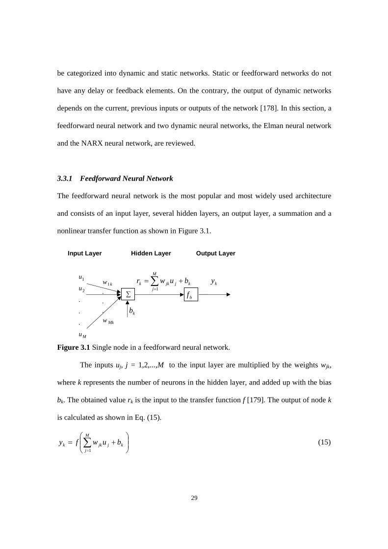
Figure 3.1 Single node in a feedforward neural network.

The inputs uj, j = 1,2,...,M to the input layer are multiplied by the weights wjk,

where k represents the number of neurons in the hidden layer, and added up with the bias

bk. The obtained value rk is the input to the transfer function f [179]. The output of node k

is calculated as shown in Eq. (15).

M

jkjjkk buwfy

1

(15)

Mu

u

u

.

.

.

2

1

hf

kb

kj

M

jjkk buwr

1ky

∑

Mk

k

w

w

.

.

.

1

30

A multi-layer feedforward (MLFF) network is structured by connecting several

nodes. A typical feedforward neural network is shown in Figure 3.2.

Figure 3.2 The architecture of feedforward neural network.

Given input data ui, i=1,2,...,Ni and output data yk, k=1,2,...,No finding the best

feedforward network can be formulated as a least squares fit by Eq. (16).

])(.[)](.[11111

Ni

iiihhh

Nh

hhoo

No

oohh

Nh

hhoo

No

ook uwbfwbfrfwbfy (16)

First, the parameters of the feedforward network architecture, namely, the number

of hidden layers and neurons in each layer need to be selected. The inputs ui, i=1,2,...,Ni to

the input neurons are multiplied by weights wih, with h=1,2,..,Nh representing the number

of neurons in the hidden layer, and summed up together with the constant bias term bh. The

resulting rh is the input to the transfer function )(hf . Later, the results of the hidden layer

are multiplied by weights who, and summed up together with the constant bias term bo. The

∑ hf

∑

hfof

of

1y

Noy

1u

2u

Hidden Units Output Units

ihw

how

.

.

....

.

.

Niu

hr

or

Input Units

hf

∑

∑

∑hb

ob

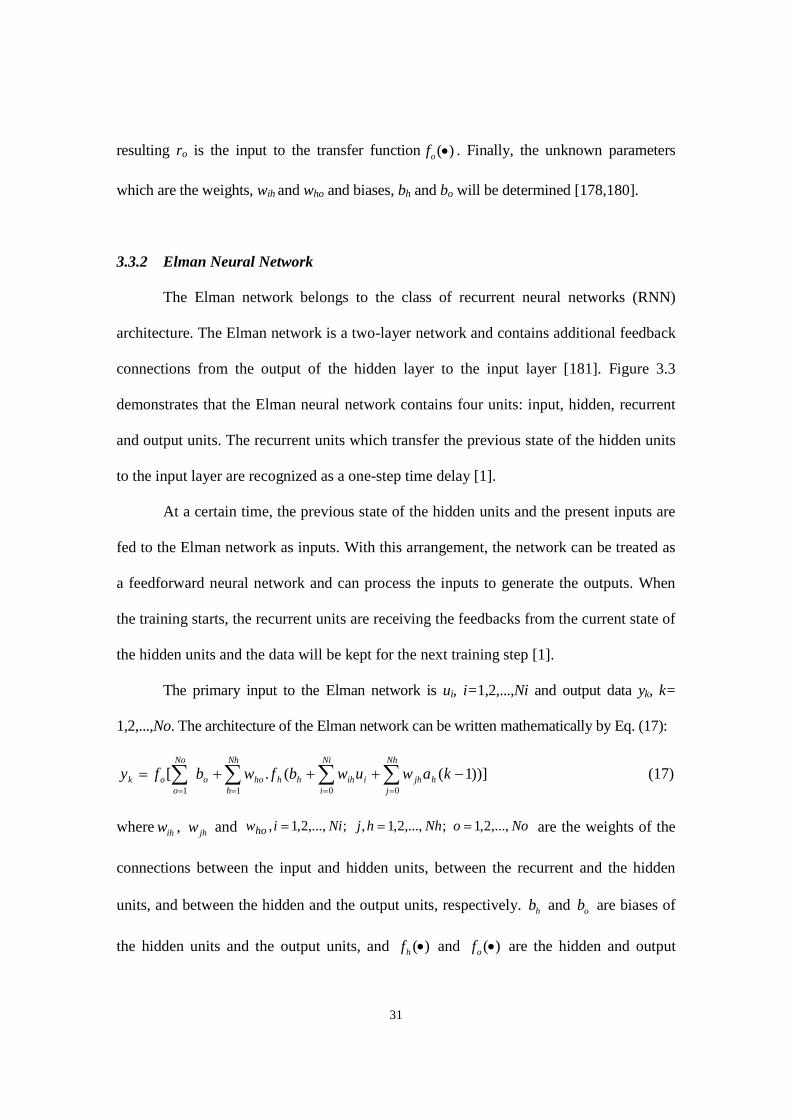
31

resulting ro is the input to the transfer function )(of . Finally, the unknown parameters

which are the weights, wih and who and biases, bh and bo will be determined [178,180].

3.3.2 Elman Neural Network

The Elman network belongs to the class of recurrent neural networks (RNN)

architecture. The Elman network is a two-layer network and contains additional feedback

connections from the output of the hidden layer to the input layer [181]. Figure 3.3

demonstrates that the Elman neural network contains four units: input, hidden, recurrent

and output units. The recurrent units which transfer the previous state of the hidden units

to the input layer are recognized as a one-step time delay [1].

At a certain time, the previous state of the hidden units and the present inputs are

fed to the Elman network as inputs. With this arrangement, the network can be treated as

a feedforward neural network and can process the inputs to generate the outputs. When

the training starts, the recurrent units are receiving the feedbacks from the current state of

the hidden units and the data will be kept for the next training step [1].

The primary input to the Elman network is ui, i=1,2,...,Ni and output data yk, k=

1,2,...,No. The architecture of the Elman network can be written mathematically by Eq. (17):

)])1((.[0 011

Ni

i

Nh

jhjhiihhh

Nh

hhoo

No

ook kawuwbfwbfy (17)

where ihw , jhw and NooNhhjNiiwho ,...,2,1;,...,2,1,;,...,2,1, are the weights of the

connections between the input and hidden units, between the recurrent and the hidden

units, and between the hidden and the output units, respectively. hb and ob are biases of

the hidden units and the output units, and )(hf and )(of are the hidden and output

32

hf

hf

hf

of

of

1y

Noy

)(1 ka

)(2 ka

)(kaNh

)1(1 ka

)1(2 ka

)1( kaNh

ob

hb

1u

2u

Niu

ihw

jhw

how

functions, respectively [1]. The structure of Eq. (17) is similar to Eq. (16) which is

generated for a feedforward neural network. However, the last term in Eq. (17),

Nh

jhjh kaw

0

)1( , represents the feedback from the hidden layer to the input layer

Figure 3.3 The architecture of Elman recurrent neural network.

3.3.3 NARX Neural Network

The nonlinear autoregressive with exogenous input (NARX) neural network is

another class of ANNs which are suitable for modeling nonlinear systems and time series

[15]. The NARX network is a dynamic neural network and contains recurrent feedback

from several layers of the network to the input layer [166,182,183]. NARX can be

mathematically represented by Eq. (18):

)](),...,();(),...,([)1( uy dnunudnynyfny (18)

∑

∑

∑

R

R

R

∑

∑

Re

cu

rre

nt

Un

its

Inp

ut

Un

its

Z-1

Z-1

Z-1

Hidden Units Output Units...

.

.

.

.

.

.

.

.

.

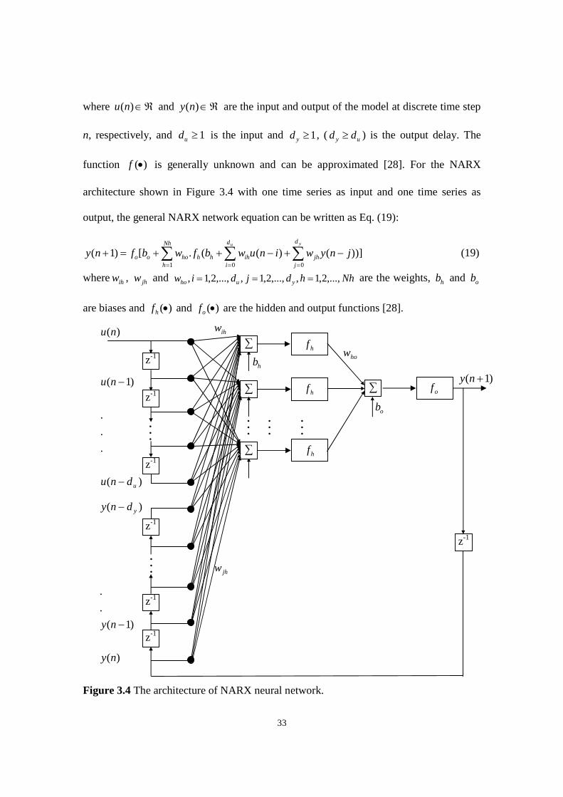
33

)(

.

.

.

)1(

)(

udnu

nu

nu

)(

)1(

.

.

)(

ny

ny

dny y

)1( nyof

hf

hf

hf

hb

ob

ihw

how

jhw

where )(nu and )(ny are the input and output of the model at discrete time step

n, respectively, and 1ud is the input and 1yd , ( uy dd ) is the output delay. The

function )(f is generally unknown and can be approximated [28]. For the NARX

architecture shown in Figure 3.4 with one time series as input and one time series as

output, the general NARX network equation can be written as Eq. (19):

)])()((.[)1(0 01

u yd

i

d

jjhihhh

Nh

hhooo jnywinuwbfwbfny (19)

where ihw , jhw and Nhhdjdiw yuho ,...,2,1,,...,2,1,,...,2,1, are the weights, hb and ob

are biases and )(hf and )(of are the hidden and output functions [28].

Figure 3.4 The architecture of NARX neural network.

z-1

z-1

z-1

z-1

z-1

z-1

z-1

.

.

.

.

.

.

∑

∑

∑

∑

.

.

....

.

.

.

34

The NARX network can be used in multi-time series input and multi-time series

output applications. The equation for a general NARX network with two inputs and one

output can be written as Eq. (20):

)])()2()1((.[)1(1 2

01 02 02211

1

u u yd

i

d

i

d

jjhhihihh

N

hhooo jnywinuwinuwbfwbfny

(20)

where hiw1 and hiw 2 , 21 ,...,2,12,,...,2,11 uu didi are the weights of the connections between

the first input units and the hidden units and between the second input units and the hidden

units, respectively [28].

3.4 Genetic Algorithms

Genetic algorithms are an evolutionary method which simulates the process of

natural selection proposed by Darwin in 1859 [184]. Genetic algorithms follow the

survival strategy used by nature to modify species. In 1975, Holland [185] introduced the

GA method for the first time for optimization purposes [70].

In the GA method, the optimization parameters are represented as strings of

binary digits to mimic biological chromosomes. Crossover and mutation are used to

generate new offspring. The format of the chromosomes is the first step in the design of

the structure of a GA search. The parameters are restructured as binary strings to form

strings of digits [70]. In GA literature, the space assigned to each parameter is called a

gene. Each gene contains several binary digits. A chromosome is formed when several

genes are combined as shown in Figure 3.5.

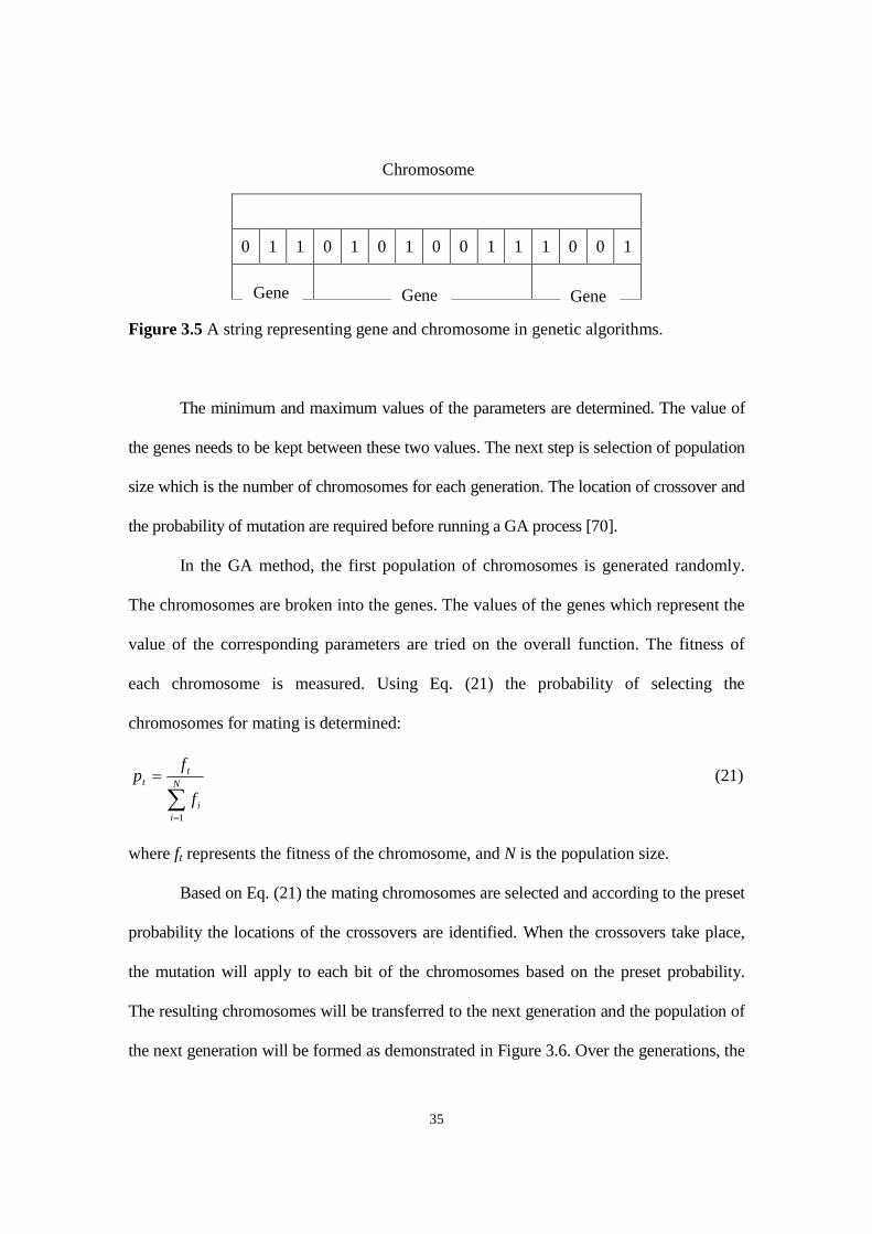
35

0 1 1 0 1 0 1 0 0 1 1 1 0 0 1

Figure 3.5 A string representing gene and chromosome in genetic algorithms.

The minimum and maximum values of the parameters are determined. The value of

the genes needs to be kept between these two values. The next step is selection of population

size which is the number of chromosomes for each generation. The location of crossover and

the probability of mutation are required before running a GA process [70].

In the GA method, the first population of chromosomes is generated randomly.

The chromosomes are broken into the genes. The values of the genes which represent the

value of the corresponding parameters are tried on the overall function. The fitness of

each chromosome is measured. Using Eq. (21) the probability of selecting the

chromosomes for mating is determined:

N

ii

tt

f

fp

1

(21)

where ft represents the fitness of the chromosome, and N is the population size.

Based on Eq. (21) the mating chromosomes are selected and according to the preset

probability the locations of the crossovers are identified. When the crossovers take place,

the mutation will apply to each bit of the chromosomes based on the preset probability.

The resulting chromosomes will be transferred to the next generation and the population of

the next generation will be formed as demonstrated in Figure 3.6. Over the generations, the

Chromosome

Gene Gene Gene

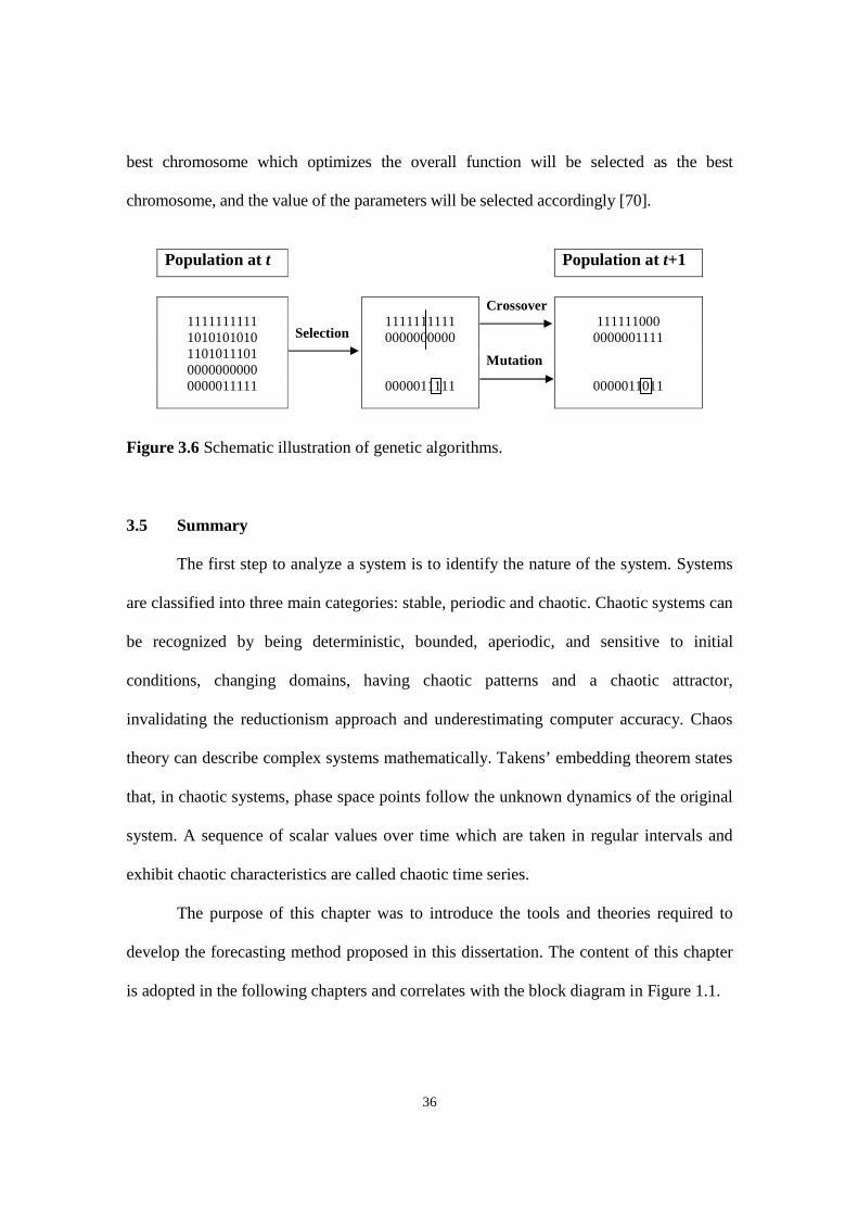
36

best chromosome which optimizes the overall function will be selected as the best

chromosome, and the value of the parameters will be selected accordingly [70].

Population at t Population at t+1

Crossover

Selection

Mutation

11111111111010101010110101110100000000000000011111

11111111110000000000

0000011111

1111110000000001111

0000011011

Figure 3.6 Schematic illustration of genetic algorithms.

3.5 Summary

The first step to analyze a system is to identify the nature of the system. Systems

are classified into three main categories: stable, periodic and chaotic. Chaotic systems can

be recognized by being deterministic, bounded, aperiodic, and sensitive to initial

conditions, changing domains, having chaotic patterns and a chaotic attractor,

invalidating the reductionism approach and underestimating computer accuracy. Chaos

theory can describe complex systems mathematically. Takens’ embedding theorem states

that, in chaotic systems, phase space points follow the unknown dynamics of the original

system. A sequence of scalar values over time which are taken in regular intervals and

exhibit chaotic characteristics are called chaotic time series.

The purpose of this chapter was to introduce the tools and theories required to

develop the forecasting method proposed in this dissertation. The content of this chapter

is adopted in the following chapters and correlates with the block diagram in Figure 1.1.

37

In Section 3.2.2, four methods, Fourier transform, Lyapunov exponent, Hurst

exponent and fractal dimension, were introduced to identify the existence of chaos in a

system. The application of Section 3.2.2 is reflected in the block diagram items 2 and 11.

Based on the content of Sections 3.2.3, 3.2.4 and 3.2.5, to apply the embedding theorem,

proper time delay and embedding dimension are required. The application of Sections

3.2.4 and 3.2.5 is mentioned in the block diagram item 3. Also, the block diagram item 4

presents the application of Section 3.2.3.

Artificial neural networks are nonlinear models which simulate the human neural

system and have the functions of self-organizing, data-driven, self-study, self-adaptive

and associated memory. ANNs are capable of capturing the hidden functional

relationships among the given data. The feedforward neural network is an example of

static neural networks and Elman and NARX are the examples of dynamic neural

networks. The content of Section 3.3 is used in the block diagram items 6 and 12. In the

block diagram item 6, the artificial neural network architectures introduced in Sections

3.3.1 and 3.3.2 can be used. In the block diagram item 12, the artificial neural network

architectures discussed in Sections 3.3.1 and 3.3.3 can be adopted.

Genetic algorithms as an evolutionary method which simulates the process of

natural selection can be used for the purpose of optimization. Genetic algorithms in

Section 3.4 can be employed to improve the result of the neural networks presented in the

block diagram items 6 and 12.

38

CHAPTER 4

COMBINATION OF CHAOS THEORY ANDARTIFICIAL INTELLIGENCE IN CHAOTIC TIMESERIES FORECASTING

In this chapter, a unique technique based on chaos theory and artificial neural networks is

proposed to analyze and forecast chaotic time series. The first requirement is to analyze

the time series and investigate the presence of chaos in the time series. The embedding

theorem is used to determine the embedding parameters D and T, and accordingly the

chaotic time series is reconstructed into the phase space points. Based on chaos theory,

there exists an unknown mathematical equation which can forecast the future value of the

phase space points. Artificial neural networks are employed to capture the functional

relationships among the given phase space points. Therefore, the embedded phase space

points are fed into a neural network and trained. The weights and biases of the trained

neural network are kept to forecast the future of phase space points. When the unknown

phase space points are predicted, the future values of the time series are obtained

consequently. Two neural network architectures, feedforward and Elman, are utilized for

forecasting. Genetic algorithms are merged with the proposed method to improve the

performance of the forecasting method by selecting the best initial weights and biases for

the neural networks. The Mackey-Glass, Logistic and Henon time series are used to

validate the performance of the proposed technique. The numerical experimental results

39

confirm that the proposed method can forecast the chaotic time series effectively and

accurately when compared with the existing forecasting methods.

The content of the current chapter has been presented at the Canadian Operational

Research Society (CORS) conference [186], published in the Proceedings of the 3rd

World Conference on Production and Operations Management [187] and accepted for

publication by the International Journal of Applied Management Science [188].

The current chapter is structured as follows. In Section 4.1, a novel forecasting

method developed in this research work, which is based on the precise definition of chaos

theory, is presented. In order to evaluate the performance of the proposed method, three

well-known chaotic time series, Mackey-Glass, Logistic and Henon are used for

benchmarking. In Section 4.2, feedforward neural network architecture is selected to

forecast the chaotic time series. In Section 4.3, Elman RNN architecture is selected to

forecast the chaotic time series. In Section 4.4, genetic algorithms are utilized to improve

the performance of the neural networks. Section 4.5 compares the performance of the

proposed forecasting method in this chapter with the results presented in similar research

works in the literature. Section 4.6 concludes Chapter 4.

4.1 Introducing the Proposed Forecasting Method

This section introduces an original technique which has been developed to forecast one

step ahead of a given chaotic time series. The current state is used to forecast the next state. When

the next state is predicted, the real value of the next state is used to forecast the following state and

so on. The key difference between this technique and the techniques proposed in the literature

[1,13] is the utilization of the precise definition of chaos theory and the embedding theorem.

40

Chaos theory states that for a chaotic system, there exists an unknown

mathematical equation which can describe the system, Eq. (2). On the other hand,

Taken’s [20] embedding theorem claims that in phase space mode, a chaotic system

reflects most of the characteristics of the original system. Therefore, s(t) in Eq. (2) can be

replaced by Y(t). Also, unknown function Q: Rn→Rn can be estimated by function G:

RD→RD where D is the embedding dimension. D mimics n, the dimension of the original

state. Eq. (2) at time t+1 can be rewritten as Eq. (22) which is the next state of the system.

)1())(()( tYtYGtY (22)

The contribution of ANN is to find an appropriate relationship between the

current state of the system and the next state of the system. In the current technique, an

artificial neural network is trained using a single phase space point (current state) as input

and a single phase space point (next state) as output. This complies precisely with the

definition of chaos theory and the embedding theorem.

On the other hand, in the forecasting methods proposed in the literature an

artificial neural network is trained either using a single phase space point as input and a

single point from the time series as output [13] or with multiple phase space points as

input and a single phase space point as output [1]. None of these approaches makes full

use of the precise definition of chaos theory.

Figure 4.1, which is Block A in Figure 1.1 demonstrates the required steps to

develop the proposed forecasting method. Based on the observed time series data set,

x(1), x(2), x(3), ..., x(N), where N is the length of the data set, the presence of chaos is

examined by Fourier transform, Lyapunov exponent, Hurst exponent and fractal

dimension as mentioned in Section 3.2.2. When the presence of chaos is detected in the

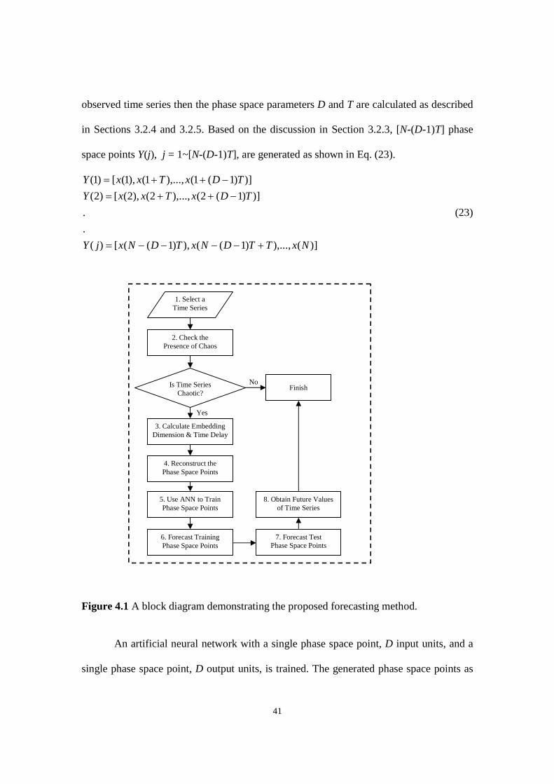
41

observed time series then the phase space parameters D and T are calculated as described

in Sections 3.2.4 and 3.2.5. Based on the discussion in Section 3.2.3, [N-(D-1)T] phase

space points Y(j), j = 1~[N-(D-1)T], are generated as shown in Eq. (23).

)](),...,)1((),)1(([)(

.

.

)])1(2(),...,2(),2([)2(

)])1(1(),...,1(),1([)1(

NxTTDNxTDNxjY

TDxTxxY

TDxTxxY

(23)

Figure 4.1 A block diagram demonstrating the proposed forecasting method.

An artificial neural network with a single phase space point, D input units, and a

single phase space point, D output units, is trained. The generated phase space points as

1. Select aTime Series

2. Check thePresence of Chaos

Is Time SeriesChaotic?

FinishNo

3. Calculate EmbeddingDimension & Time Delay

Yes

4. Reconstruct thePhase Space Points

5. Use ANN to TrainPhase Space Points

6. Forecast TrainingPhase Space Points

7. Forecast TestPhase Space Points

8. Obtain Future Valuesof Time Series

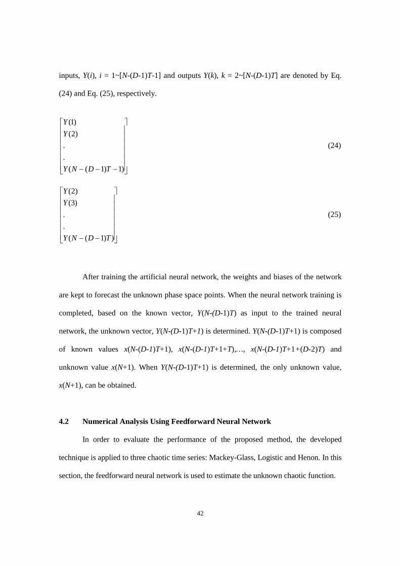
42

inputs, Y(i), i = 1~[N-(D-1)T-1] and outputs Y(k), k = 2~[N-(D-1)T] are denoted by Eq.

(24) and Eq. (25), respectively.

)1)1((

.

.

)2(

)1(

TDNY

Y

Y

(24)

))1((

.

.

)3(

)2(

TDNY

Y

Y

(25)

After training the artificial neural network, the weights and biases of the network

are kept to forecast the unknown phase space points. When the neural network training is

completed, based on the known vector, Y(N-(D-1)T) as input to the trained neural

network, the unknown vector, Y(N-(D-1)T+1) is determined. Y(N-(D-1)T+1) is composed

of known values x(N-(D-1)T+1), x(N-(D-1)T+1+T),…, x(N-(D-1)T+1+(D-2)T) and

unknown value x(N+1). When Y(N-(D-1)T+1) is determined, the only unknown value,

x(N+1), can be obtained.

4.2 Numerical Analysis Using Feedforward Neural Network

In order to evaluate the performance of the proposed method, the developed

technique is applied to three chaotic time series: Mackey-Glass, Logistic and Henon. In this

section, the feedforward neural network is used to estimate the unknown chaotic function.

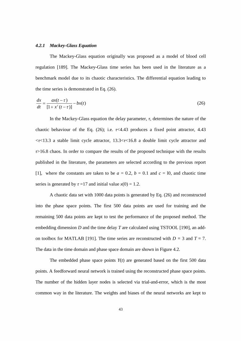
43

4.2.1 Mackey-Glass Equation

The Mackey-Glass equation originally was proposed as a model of blood cell

regulation [189]. The Mackey-Glass time series has been used in the literature as a

benchmark model due to its chaotic characteristics. The differential equation leading to

the time series is demonstrated in Eq. (26).

)()](1[

)(tbx

tx

tax

dt

dxc

(26)

In the Mackey-Glass equation the delay parameter, τ, determines the nature of the

chaotic behaviour of the Eq. (26); i.e. τ<4.43 produces a fixed point attractor, 4.43

<τ<13.3 a stable limit cycle attractor, 13.3<τ<16.8 a double limit cycle attractor and

τ>16.8 chaos. In order to compare the results of the proposed technique with the results

published in the literature, the parameters are selected according to the previous report

[1], where the constants are taken to be a = 0.2, b = 0.1 and c = l0, and chaotic time

series is generated by τ =17 and initial value x(0) = 1.2.

A chaotic data set with 1000 data points is generated by Eq. (26) and reconstructed

into the phase space points. The first 500 data points are used for training and the

remaining 500 data points are kept to test the performance of the proposed method. The

embedding dimension D and the time delay T are calculated using TSTOOL [190], an add-

on toolbox for MATLAB [191]. The time series are reconstructed with D = 3 and T = 7.

The data in the time domain and phase space domain are shown in Figure 4.2.

The embedded phase space points Y(t) are generated based on the first 500 data

points. A feedforward neural network is trained using the reconstructed phase space points.

The number of the hidden layer nodes is selected via trial-and-error, which is the most

common way in the literature. The weights and biases of the neural networks are kept to

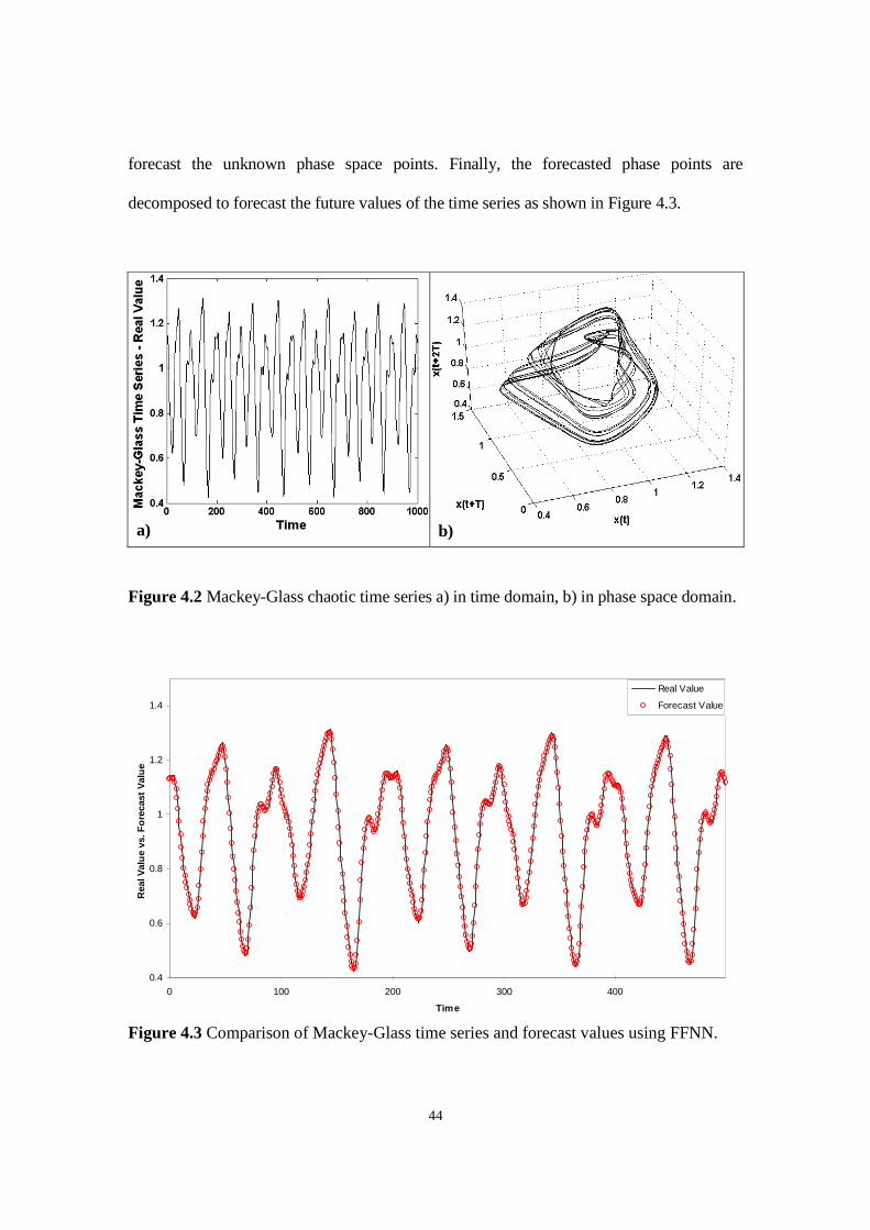
44

forecast the unknown phase space points. Finally, the forecasted phase points are

decomposed to forecast the future values of the time series as shown in Figure 4.3.

Figure 4.2 Mackey-Glass chaotic time series a) in time domain, b) in phase space domain.

0.4

0.6

0.8

1

1.2

1.4

0 100 200 300 400

Time

RealV

alu

evs.F

ore

cast

Valu

e

Real Value

Forecast Value

Figure 4.3 Comparison of Mackey-Glass time series and forecast values using FFNN.

a) b)

45

Based on the selected research works for comparison, the error indices are

calculated. In order to evaluate the prediction performance and compare it with the results

reported in the literature, the mean squared error (MSE) and the normalized mean

squared error (NMSE) are calculated by Eq. (27) and Eq. (28), respectively.

N

iii yy

NMSE

1

2)(1

(27)

N

ii

N

iii

yy

yy

NMSE

1

2

1

2

)(

)(

(28)

where iy , iy

and y are observed data, predicted data and the average of observed data,

respectively, and N is the length of observed data. The MSE and NMSE values are

reflected in Table 4.1. Appendix D exhibits the regression analysis between the network

response and the corresponding targets for the feedforward neural network.

Table 4.1 Mackey-Glass time series – The MSE and NMSE for the 500 test samples.

Prediction Error

Prediction Method Reference MSE NMSE

Proposed Method – FFNN 5.98E-05 1.20E-03

4.2.2 Logistic Equation

The Logistic equation is the most famous, oldest and simplest chaotic

mathematical system [70,171,192]. Although it has only one control parameter and one

variable, it demonstrates chaotic behaviour. The Logistic equation had been used in insect

studies [193] and fish population growth [194], however, physicist and mathematical

biologist May [195] revealed the importance of the Logistic equation [171] as a chaotic

system. The Logistic equation is written as Eq. (29).

46

)](1)[()1( txtrxtx (29)

With an initial state of x(0) = 0.36 and r = 4.0, a chaotic time series with 612 data

points is generated using Eq. (29). The data in the time domain is shown in Figure 4.4.

The embedding dimension D = 3 and the time delay T = 1 are selected based on Zhang et

al. [196] and the time series is reconstructed.

Figure 4.4 Logistic chaotic time series a) in time domain, b) in phase space domain.

The embedded phase space points Y(t) are obtained based on the first 512 data

points. The feedforward neural network is trained using the phase space points. The

remaining 100 data points are kept to examine the performance of the proposed

forecasting method. The weights and biases are kept to forecast the unknown phase space

points and consequently the future values of the time series as shown in Figure 4.5.

The MSE and NMSE are calculated to evaluate the performance of the proposed

method when applied to the Logistic time series and shown in Table 4.2. Appendix D

exhibits the regression analysis between the network response and the corresponding

targets for feedforward neural networks.

a) b)

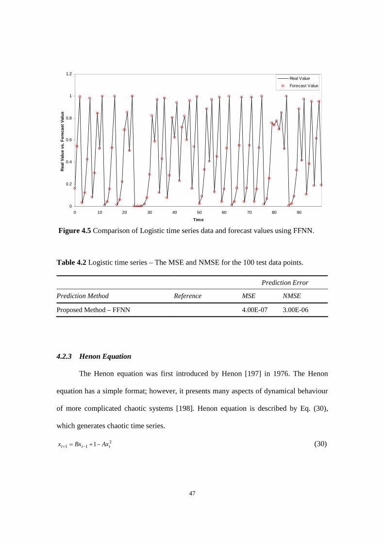
47

0

0.2

0.4

0.6

0.8

1

1.2

0 10 20 30 40 50 60 70 80 90

Time

RealV

alu

evs.F

ore

cast

Valu

e

Real Value

Forecast Value

Figure 4.5 Comparison of Logistic time series data and forecast values using FFNN.

Table 4.2 Logistic time series – The MSE and NMSE for the 100 test data points.

Prediction Error


Proposed Method – FFNN 4.00E-07 3.00E-06

4.2.3 Henon Equation

The Henon equation was first introduced by Henon [197] in 1976. The Henon

equation has a simple format; however, it presents many aspects of dynamical behaviour

of more complicated chaotic systems [198]. Henon equation is described by Eq. (30),

which generates chaotic time series.

211 1 ttt AxBxx (30)

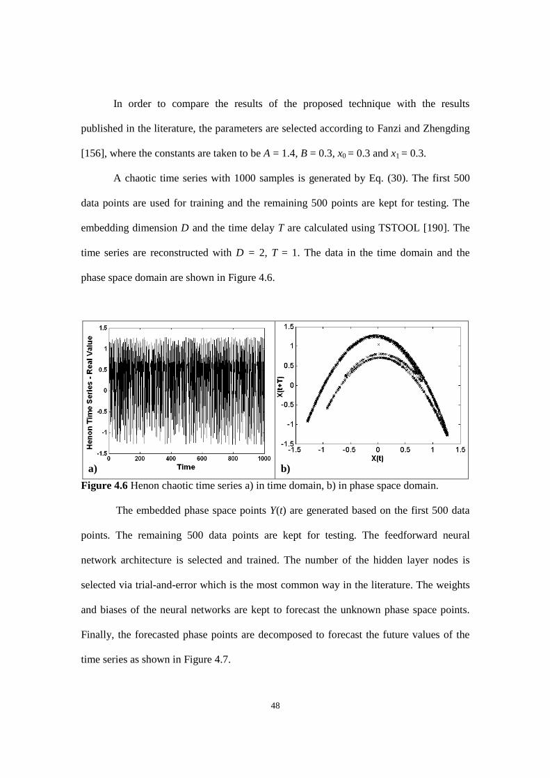
48

In order to compare the results of the proposed technique with the results

published in the literature, the parameters are selected according to Fanzi and Zhengding

[156], where the constants are taken to be A = 1.4, B = 0.3, x0 = 0.3 and x1 = 0.3.

A chaotic time series with 1000 samples is generated by Eq. (30). The first 500

data points are used for training and the remaining 500 points are kept for testing. The

embedding dimension D and the time delay T are calculated using TSTOOL [190]. The

time series are reconstructed with D = 2, T = 1. The data in the time domain and the

phase space domain are shown in Figure 4.6.

Figure 4.6 Henon chaotic time series a) in time domain, b) in phase space domain.

The embedded phase space points Y(t) are generated based on the first 500 data

points. The remaining 500 data points are kept for testing. The feedforward neural

network architecture is selected and trained. The number of the hidden layer nodes is

selected via trial-and-error which is the most common way in the literature. The weights

and biases of the neural networks are kept to forecast the unknown phase space points.

Finally, the forecasted phase points are decomposed to forecast the future values of the

time series as shown in Figure 4.7.

a) b)

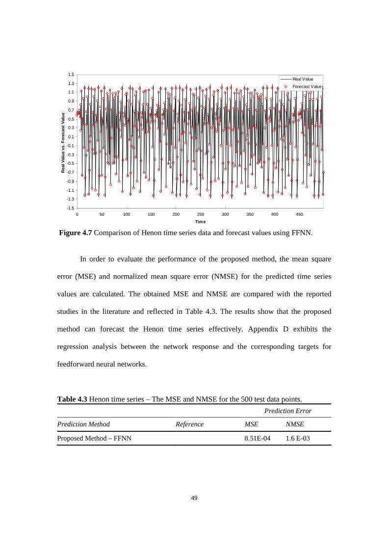
49

-1.5

-1.3

-1.1

-0.9

-0.7

-0.5

-0.3

-0.1

0.1

0.3

0.5

0.7

0.9

1.1

1.3

1.5

0 50 100 150 200 250 300 350 400 450

Time

RealV

alu

evs.F

ore

cast

Valu

e

Real Value

Forecast Value

Figure 4.7 Comparison of Henon time series data and forecast values using FFNN.

In order to evaluate the performance of the proposed method, the mean square

error (MSE) and normalized mean square error (NMSE) for the predicted time series

values are calculated. The obtained MSE and NMSE are compared with the reported

studies in the literature and reflected in Table 4.3. The results show that the proposed

method can forecast the Henon time series effectively. Appendix D exhibits the

regression analysis between the network response and the corresponding targets for

feedforward neural networks.

Table 4.3 Henon time series – The MSE and NMSE for the 500 test data points.

Prediction Error


Proposed Method – FFNN 8.51E-04 1.6 E-03

50

4.3 Numerical Analysis Using Elman Neural Network

The experiments in Section 4.2 which are performed with a feedforward neural

network are repeated with an Elman recurrent neural network. The conditions are kept the

same to be able to compare the results. The only difference between the Elman recurrent

network and the feedforward neural network is the feedback mechanism which transfers

the information in hidden layer to the input layer. Figure 4.8, Figure 4.9 and Figure 4.10

exhibit the outcomes of the proposed forecasting method when applied to the Mackey-

Glass (M-G), Logistic and Henon time series using the Elman recurrent network.

Table 4.4 presents the performance of the proposed forecasting method using the

Elman recurrent network for the three chaotic time series: Mackey-Glass, Logistic and

Henon. Appendix D exhibits the regression analysis between the network response and

the corresponding targets for Elman neural networks.

0.4

0.6

0.8

1

1.2

1.4

0 100 200 300 400

Time

RealV

alu

evs.F

ore

cast

Valu

e

Real Value

Forecast Value

Figure 4.8 Comparison of M-G time series data and forecast values using Elman ANN.

51

0

0.2

0.4

0.6

0.8

1

1.2

0 10 20 30 40 50 60 70 80 90

Time

RealV

alu

evs.F

ore

cast

Valu

e

Real Value

Forecast Value

Figure 4.9 Comparison of Logistic time series data and forecast values using Elman RNN.

-1.5

-1.3

-1.1

-0.9

-0.7

-0.5

-0.3

-0.1

0.1

0.3

0.5

0.7

0.9

1.1

1.3

1.5

0 50 100 150 200 250 300 350 400 450

Time

RealV

alu

evs

.F

ore

cast

Valu

e

Real Value

Forecast Value

Figure 4.10 Comparison of Henon time series data and forecast values using Elman RNN.

52

Table 4.4 The prediction performance using Elman RNN.

Prediction Error

Time Series MSE NMSE

Mackey-Glass 4.12E-05 8.05E-04

Logistic 2.44E-11 1.89E-10

Henon 5.41E-09 1.01E-08

4.4 Improving the Results Using Genetic Algorithms

In most training algorithms, the initial weights and biases of the neural network are

selected randomly. This will cause variation in the output of the neural network. To reduce

the variation of the neural network output and improve the performance of the prediction,

genetic algorithms (GA) are adopted to find appropriate initial weights and biases. The GA

objective function is to minimize the mean square error (MSE) between the predicted values

and the original values. The GA variables are weights and biases of the neural network.

When the GA is applied, the best weights and biases which improve MSE are selected.

Table 4.5 presents the performance of the proposed forecasting method improved

by genetic algorithms for both feedforward and Elman recurrent neural networks when

applied to the three chaotic time series: Mackey-Glass, Logistic and Henon.

Table 4.5 The prediction performance improved by genetic algorithms.

Prediction Error

Time Series MSE NMSE

Mackey-Glass – Feedforward 5.24E-05 1.0E-03

Mackey-Glass – Elman 3.67E-05 7.16E-04

Logistic – Feedforward 2.54E-08 1.90E-07

Logistic – Elman 1.62E-11 1.21E-10

Henon – Feedforward 6.53E-04 1.20E-03

Henon – Elman 4.76E-09 9.01E-09

53

4.5 Comparing the Results

The results obtained in this chapter based on the proposed method are compared

with the results presented in the literature. For the Mackey-Glass time series, the

performance of the proposed method in this chapter is compared with the results of a

simple feedforward neural network and the methods delivered by Zhang and Man [1] and

Zhang et al. [39]. The method suggested by Zhang et al. [39] utilizes the application of the

delay coordinate embedding technique in the multi-input multi-output adaptive-network-

based fuzzy inference system (MANFIS) to forecast chaotic time series. Zhang and Man

[1] used an Elman recurrent neural network to forecast chaotic time series. To improve

their results, Zhang and Man [1] proposed a multi-dimensional method which combines the

output of several trained neural networks with different embedding dimensions.

Table 4.6 compares the performance of the proposed method with the results

presented in the literature. Based on this comparison, the proposed method using an Elman

recurrent neural network and improved by genetic algorithms shows better performance.

Table 4.6 Mackey-Glass time series – comparing the prediction performance.

Prediction Error


Neuro-Fuzzy [39] 1.26E-03

RNN – D = 2 [1] 1.02E-03

RNN – D = 3 [1] 4.15E-04

RNN – Multi-dimension [1] 3.81E-04

Simple Feedforward 9.75E-04 1.9E-02

Proposed method – Elman 4.12E-05 8.05E-04

Proposed method – Elman & GA 3.67E-05 7.16E-04

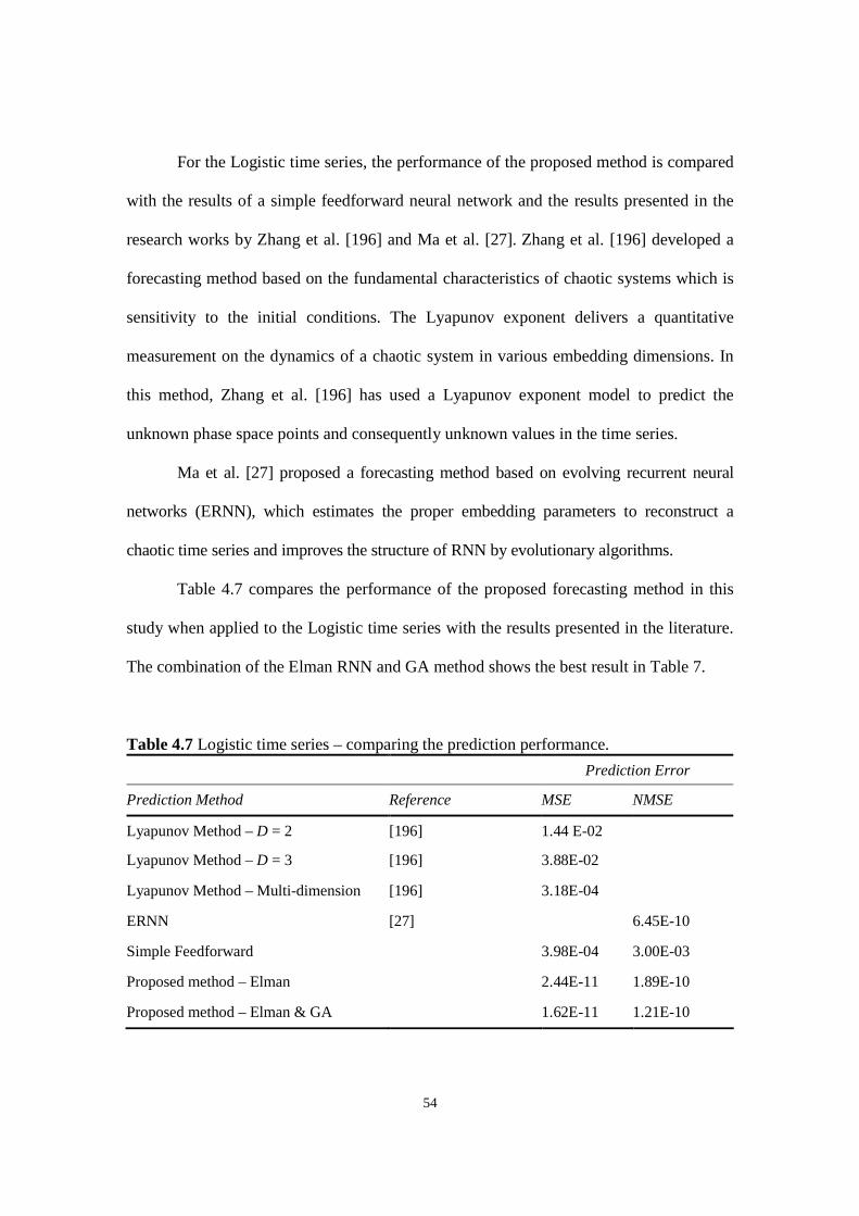
54

For the Logistic time series, the performance of the proposed method is compared

with the results of a simple feedforward neural network and the results presented in the

research works by Zhang et al. [196] and Ma et al. [27]. Zhang et al. [196] developed a

forecasting method based on the fundamental characteristics of chaotic systems which is

sensitivity to the initial conditions. The Lyapunov exponent delivers a quantitative

measurement on the dynamics of a chaotic system in various embedding dimensions. In

this method, Zhang et al. [196] has used a Lyapunov exponent model to predict the

unknown phase space points and consequently unknown values in the time series.

Ma et al. [27] proposed a forecasting method based on evolving recurrent neural

networks (ERNN), which estimates the proper embedding parameters to reconstruct a

chaotic time series and improves the structure of RNN by evolutionary algorithms.

Table 4.7 compares the performance of the proposed forecasting method in this

study when applied to the Logistic time series with the results presented in the literature.

The combination of the Elman RNN and GA method shows the best result in Table 7.

Table 4.7 Logistic time series – comparing the prediction performance.

Prediction Error


Lyapunov Method – D = 2 [196] 1.44 E-02

Lyapunov Method – D = 3 [196] 3.88E-02

Lyapunov Method – Multi-dimension [196] 3.18E-04

ERNN [27] 6.45E-10




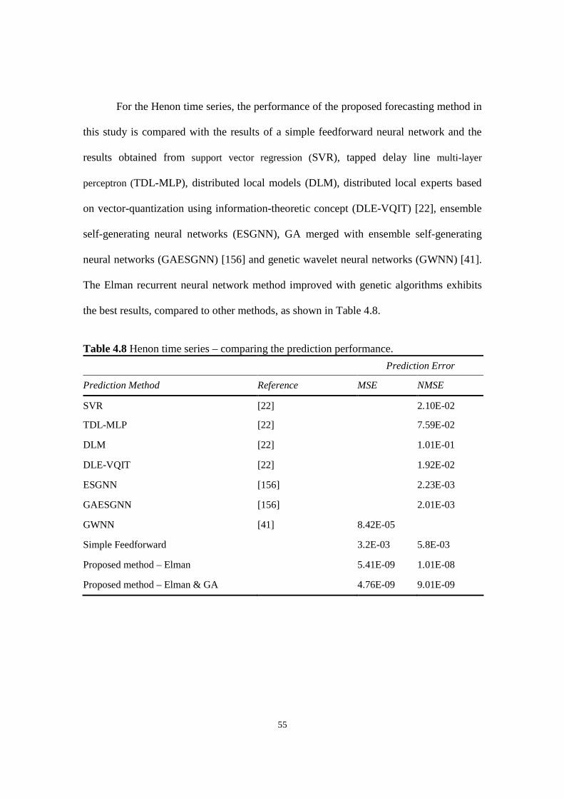
55

For the Henon time series, the performance of the proposed forecasting method in

this study is compared with the results of a simple feedforward neural network and the

results obtained from support vector regression (SVR), tapped delay line multi-layer

perceptron (TDL-MLP), distributed local models (DLM), distributed local experts based

on vector-quantization using information-theoretic concept (DLE-VQIT) [22], ensemble

self-generating neural networks (ESGNN), GA merged with ensemble self-generating

neural networks (GAESGNN) [156] and genetic wavelet neural networks (GWNN) [41].

The Elman recurrent neural network method improved with genetic algorithms exhibits

the best results, compared to other methods, as shown in Table 4.8.

Table 4.8 Henon time series – comparing the prediction performance.

Prediction Error


SVR [22] 2.10E-02

TDL-MLP [22] 7.59E-02

DLM [22] 1.01E-01

DLE-VQIT [22] 1.92E-02

ESGNN [156] 2.23E-03

GAESGNN [156] 2.01E-03

GWNN [41] 8.42E-05




56

4.6 Summary

In this chapter, a combination of chaos theory and neural networks is used to

develop a new technique to forecast chaotic time series. The phase space reconstruction

method is employed to reconstruct phase space points from chaotic time series using

embedding dimension D and time delay T. According to the phase space reconstruction

method, the phase space points will reproduce the key characteristics of the original time

series. Artificial neural networks which can capture the relationships among the data

where the underlying function is unknown or difficult to determine have been utilized to

forecast the future value of phase space points and consequently the chaotic time series.

The feedforward and Elman neural networks are selected for one step ahead

forecasting. The developed technique has been applied to three different chaotic time

series, Mackey-Glass, Logistic and Henon, to validate the effectiveness of the proposed

technique. The proposed method is merged with genetic algorithms to improve the

forecasting results. It has been observed that the new forecasting method improved with

GA presents an outstanding result. The comparison between the result of the proposed

technique and the results reported in the literature substantiates the effectiveness of the

proposed method.

57

CHAPTER 5

CHAOTIC TIME SERIES FORECASTING WITHRESIDUAL ANALYSIS USING ENSEMBLENEURAL NETWORKS

In this chapter, the contribution of residual analysis to improve the performance of the

proposed forecasting method in Chapter 4 is investigated. A combination of the embedding

theorem, artificial neural networks, residual analysis and genetic algorithms is employed to

develop an effective technique to forecast chaotic time series. Similar to the previous

method, the embedding theorem is utilized to unfold the chaotic time series and reconstruct

the phase space points. The first artificial neural network is trained to forecast the future

values of the phase space points and accordingly the original time series.

In the new approach, the residuals of the predicted time series are analyzed. In

some events, the residuals show a high degree of correlation and demonstrate chaotic

behaviour. Therefore, the residuals are considered as a new chaotic time series and

reconstructed according to the embedding theorem. A new neural network is trained to

predict the future values of the residual time series. The residual analysis can be repeated

several times. Finally, a neural network is trained using the neural networks’ result values

of the time series and the residuals as input and the original time series as output. The last

neural network is used to capture the relationship between the outcome of neural

networks and the original time series. The weights and biases of the final artificial neural

58

network are kept to predict the future values of the original time series. Two different

configurations are considered in the selection of artificial neural network combinations.

In the first configuration, all the selected neural networks are feedforward neural

networks. In the second configuration, the combination of Elman and NARX neural

networks is selected. The new proposed forecasting method is applied to the Mackey-

Glass and Lorenz equations which produce chaotic time series, and to a real life chaotic

time series, sunspot time series, to evaluate the validity of the proposed technique. The

experimental results confirm that the proposed method can predict the chaotic time series

more effectively and accurately when compared with the existing prediction methods.

The content of the current chapter has been presented at the 29th International

Symposium on Forecasting [199], submitted to Applied Artificial Intelligence Journal

[200], and published in the Proceedings of the Industrial Engineering Research

Conference [201] and the journal of Neurocomputing [202].

5.1 Introducing Residual Analysis Method

Heuristic models which are developed to predict time series mainly overlook the

characteristics of the residuals. In some cases, heuristic models cannot completely

capture the characteristics of the original time series, and the residuals show a high

correlation. The high correlation of the residuals means that prediction errors are not due

to randomness. This study considers this crucial finding and this section introduces a new

technique which employs a combination of the embedding theorem, artificial neural

networks, genetic algorithms and residual analysis to develop more effective method to

forecast one step ahead of a chaotic time series.

59

Figure 1.1 shows the block diagram demonstrating the proposed methodology in

this chapter. Block A in Figure 1.1 is discussed earlier in Chapter 4. it proposes a

forecasting method based on the embedding theorem and artificial neural networks.

Block B in Figure 1.1 proposes a new approach to enhance the results of the forecasting

method proposed in Chapter 4.

According to the Block A in Figure 1.1, the existence of chaos is investigated in the

observed time series data set, x(1), x(2), x(3), ..., x(N), where N is the length of the data set.

When the presence of chaos is detected in the observed time series, then the phase space

parameters, embedding dimension D and time delay T, are calculated. Based on the

discussion in Section 3.2.3, the phase space points are generated. An artificial neural

network with a single phase space point, D input units, and a single phase space point, D

output units, is trained. After training the artificial neural network, the weights and biases

of the network are kept to forecast the unknown phase space points. Finally the future

values of the time series are obtained.

So far, one step ahead of the original time series is predicted. As mentioned earlier,

in some cases heuristic models cannot completely capture the characteristics of the original

time series and therefore, the residuals are highly correlated. The residuals resulting from

the developed prediction method are analyzed, and it has been observed that in some cases

they demonstrate chaotic behaviour.

To investigate the contribution of the residual analysis in improving the

performance and accuracy of the proposed prediction method, the obtained residuals are

considered as a new chaotic time series and analyzed separately. Block B in Figure 1.1

demonstrates the required steps to analyze and incorporate the residuals into the proposed

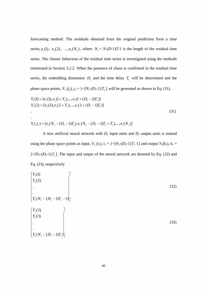
60

forecasting method. The residuals obtained from the original prediction form a time

series, )1(1e , )2(1e , ..., )( 11 Ne , where 1N = N-(D-1)T-1 is the length of the residual time

series. The chaotic behaviour of the residual time series is investigated using the methods

mentioned in Section 3.2.2. When the presence of chaos is confirmed in the residual time

series, the embedding dimension 1D and the time delay 1T will be determined and the

phase space points, Y1 (j1), j1 = 1~[N1-(D1-1) 1T ], will be generated as shown in Eq. (31).

)](),...,)1((),)1(([)(

.

.

)])1(2(),...,2(),2([)2(

)])1(1(),...,1(),1([)1(

1111111111111

1111111

1111111

NeTTDNeTDNejY

TDeTeeY

TDeTeeY

(31)

A new artificial neural network with D1 input units and D1 output units is trained

using the phase space points as input, Y1 (i1), i1 = 1~[N1-(D1-1) 1T -1] and output Y1(k1), k1 =

2~[N1-(D1-1) 1T ]. The input and output of the neural network are denoted by Eq. (32) and

Eq. (33), respectively

)1)1((

.

.

)2(

)1(

1111

1

1

TDNY

Y

Y

(32)

))1((

.

.

)3(

)2(

1111

1

1

TDNY

Y

Y

(33)

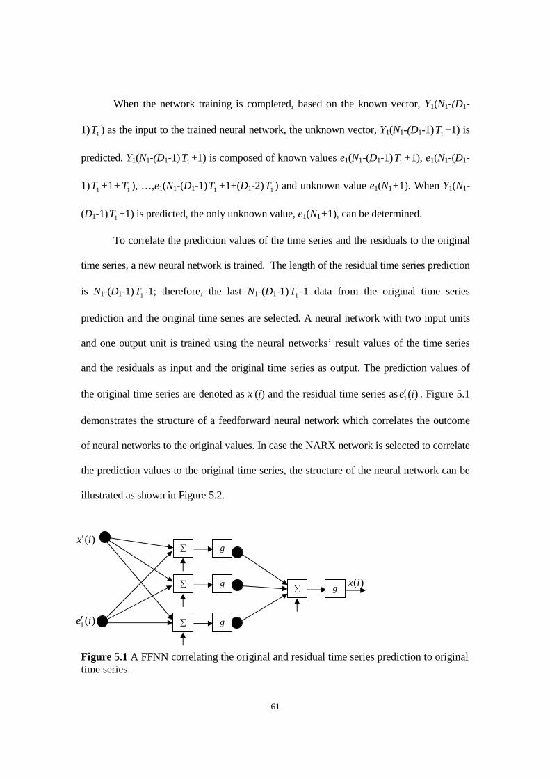
61

When the network training is completed, based on the known vector, Y1(N1-(D1-

1) 1T ) as the input to the trained neural network, the unknown vector, Y1(N1-(D1-1) 1T +1) is

predicted. Y1(N1-(D1-1) 1T +1) is composed of known values e1(N1-(D1-1) 1T +1), e1(N1-(D1-

1) 1T +1+ 1T ), …,e1(N1-(D1-1) 1T +1+(D1-2) 1T ) and unknown value e1(N1+1). When Y1(N1-

(D1-1) 1T +1) is predicted, the only unknown value, e1(N1+1), can be determined.

To correlate the prediction values of the time series and the residuals to the original

time series, a new neural network is trained. The length of the residual time series prediction

is N1-(D1-1) 1T -1; therefore, the last N1-(D1-1) 1T -1 data from the original time series

prediction and the original time series are selected. A neural network with two input units

and one output unit is trained using the neural networks’ result values of the time series

and the residuals as input and the original time series as output. The prediction values of

the original time series are denoted as x'(i) and the residual time series as )(1 ie . Figure 5.1

demonstrates the structure of a feedforward neural network which correlates the outcome

of neural networks to the original values. In case the NARX network is selected to correlate

the prediction values to the original time series, the structure of the neural network can be

illustrated as shown in Figure 5.2.

Figure 5.1 A FFNN correlating the original and residual time series prediction to originaltime series.

)(

)(

1 ie

ix

∑

)(ix∑

∑

g

g

g

∑ g

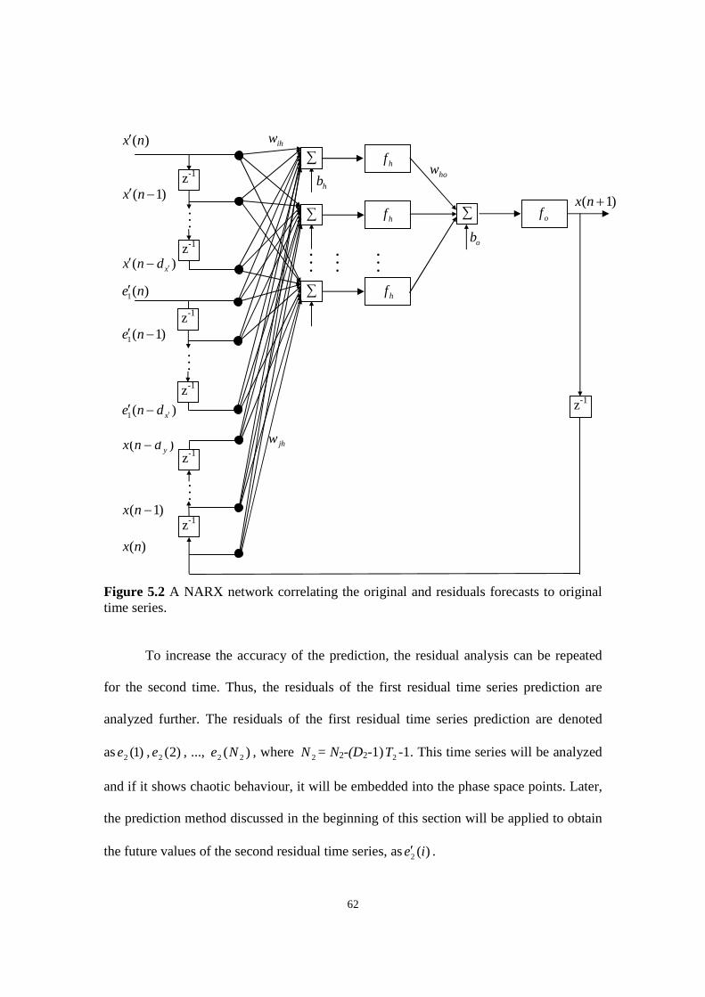
62

)(nx

)( ydnx

)1( nxof

hf

hf

hf

hb

ob

ihw

how

jhw

)( xdnx

)1( nx

)(nx

)1( nx

)(1 ne

)(1 xdne

)1(1 ne

Figure 5.2 A NARX network correlating the original and residuals forecasts to originaltime series.

To increase the accuracy of the prediction, the residual analysis can be repeated

for the second time. Thus, the residuals of the first residual time series prediction are

analyzed further. The residuals of the first residual time series prediction are denoted

as )1(2e , )2(2e , ..., )( 22 Ne , where 2N = N2-(D2-1) 2T -1. This time series will be analyzed

and if it shows chaotic behaviour, it will be embedded into the phase space points. Later,

the prediction method discussed in the beginning of this section will be applied to obtain

the future values of the second residual time series, as )(2 ie .

z-1

z-1

z-1

z-1

z-1

.

.

.

.

.

.

∑

∑

∑

∑

.

.

....

.

.

.

z-1

z-1

.

.

.

63

The residual analysis can be repeated several times. To correlate the neural

networks’ result values of the time series and the residuals in various levels to the

original time series, a neural network with M+1 input units, where M is the level of

residual analysis, and one output unit can be trained. Figure 5.3 demonstrates the

structure of the final neural network with M level of residual analysis which correlates the

prediction values to the original values. The proposed method is merged with genetic

algorithms to improve the forecasting results.

Figure 5.3 A FFNN correlating the original time series prediction and the prediction ofresiduals in various levels to original time series.

5.2 Numerical Analysis Using Feedforward-Feedforward Configuration

In this section, the unique approach developed in this chapter using feedforward-

feedforward neural network configuration is applied to two simulated chaotic systems:

Mackey-Glass and Lorenz equations.


The details of the Mackey-Glass equation have been presented in Section 4.2.1.

Similar to Section 4.2.1, the parameters in Eq. (26) are selected according to the previous

report by Zhang and Man [1], where the constants are taken to be a = 0.2, b = 0.1 and c = l0

and chaotic time series is generated by time delay τ =17 and initial value x(0) = 1.2.

)(

.

.

.

)(

)(

1

ie

ie

ix

M

∑

)(ix∑

∑

g

g

g

∑ g

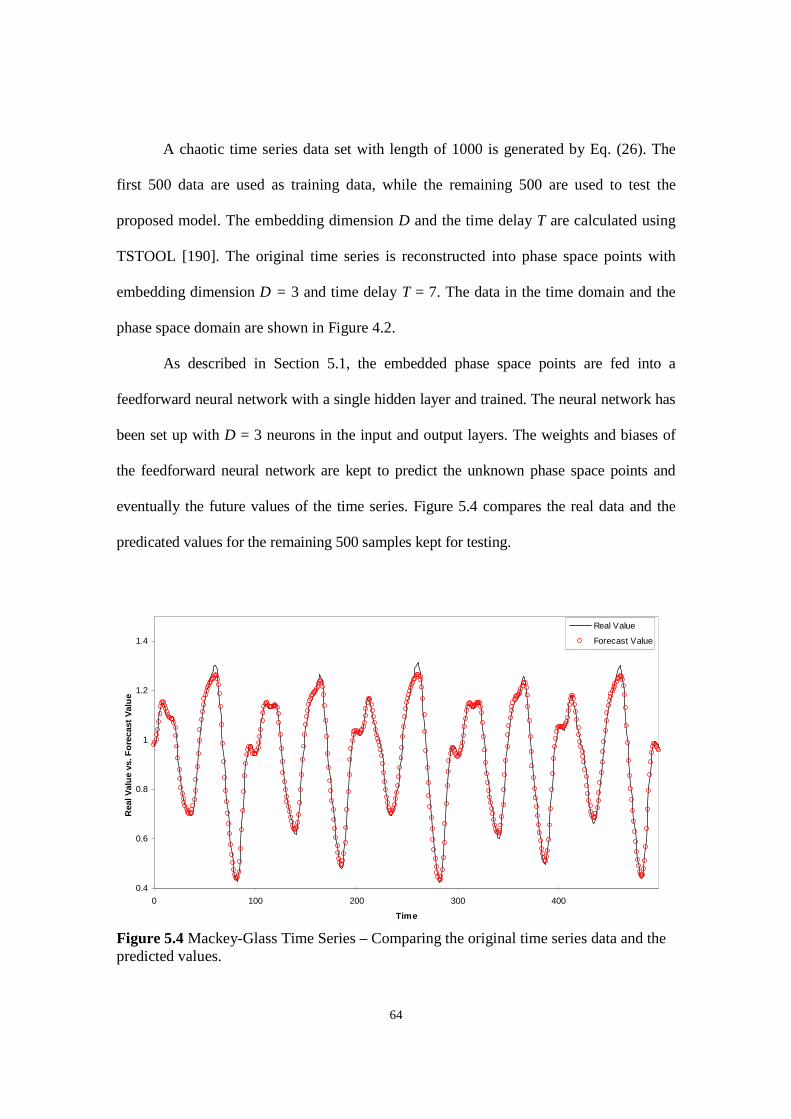
64

A chaotic time series data set with length of 1000 is generated by Eq. (26). The

first 500 data are used as training data, while the remaining 500 are used to test the

proposed model. The embedding dimension D and the time delay T are calculated using

TSTOOL [190]. The original time series is reconstructed into phase space points with

embedding dimension D = 3 and time delay T = 7. The data in the time domain and the

phase space domain are shown in Figure 4.2.

As described in Section 5.1, the embedded phase space points are fed into a

feedforward neural network with a single hidden layer and trained. The neural network has

been set up with D = 3 neurons in the input and output layers. The weights and biases of

the feedforward neural network are kept to predict the unknown phase space points and

eventually the future values of the time series. Figure 5.4 compares the real data and the

predicated values for the remaining 500 samples kept for testing.

0.4

0.6

0.8

1

1.2

1.4

0 100 200 300 400

Time

RealV

alu

evs.F

ore

cast

Valu

e

Real Value

Forecast Value

Figure 5.4 Mackey-Glass Time Series – Comparing the original time series data and thepredicted values.

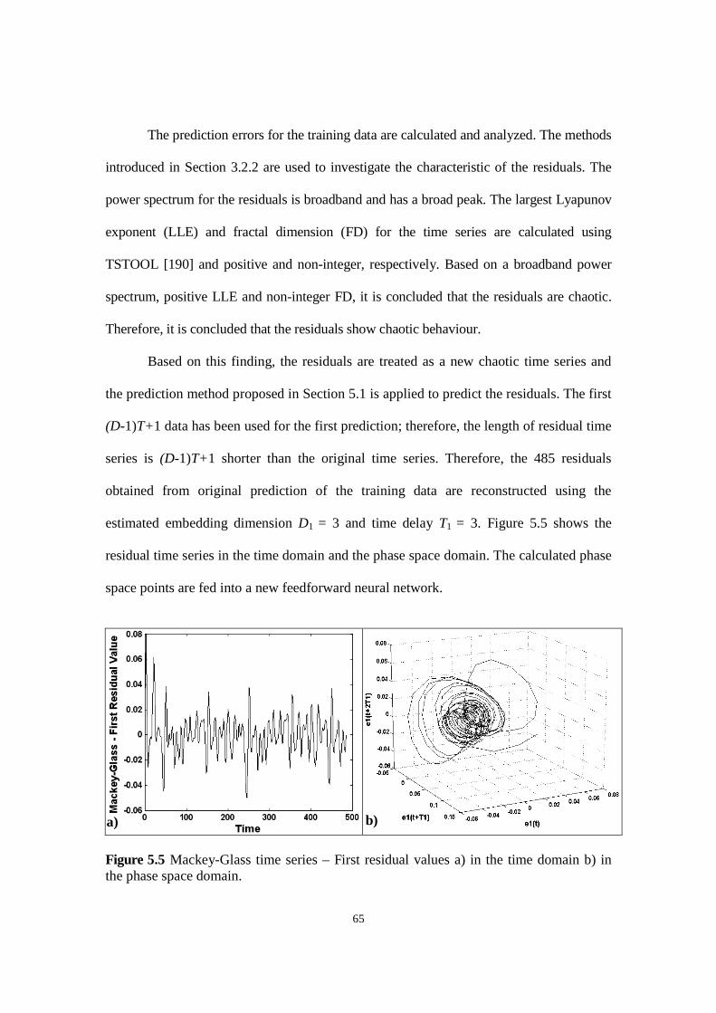
65

The prediction errors for the training data are calculated and analyzed. The methods

introduced in Section 3.2.2 are used to investigate the characteristic of the residuals. The

power spectrum for the residuals is broadband and has a broad peak. The largest Lyapunov

exponent (LLE) and fractal dimension (FD) for the time series are calculated using

TSTOOL [190] and positive and non-integer, respectively. Based on a broadband power

spectrum, positive LLE and non-integer FD, it is concluded that the residuals are chaotic.

Therefore, it is concluded that the residuals show chaotic behaviour.

Based on this finding, the residuals are treated as a new chaotic time series and

the prediction method proposed in Section 5.1 is applied to predict the residuals. The first

(D-1)T+1 data has been used for the first prediction; therefore, the length of residual time

series is (D-1)T+1 shorter than the original time series. Therefore, the 485 residuals

obtained from original prediction of the training data are reconstructed using the

estimated embedding dimension D1 = 3 and time delay T1 = 3. Figure 5.5 shows the

residual time series in the time domain and the phase space domain. The calculated phase

space points are fed into a new feedforward neural network.

Figure 5.5 Mackey-Glass time series – First residual values a) in the time domain b) inthe phase space domain.

a) b)

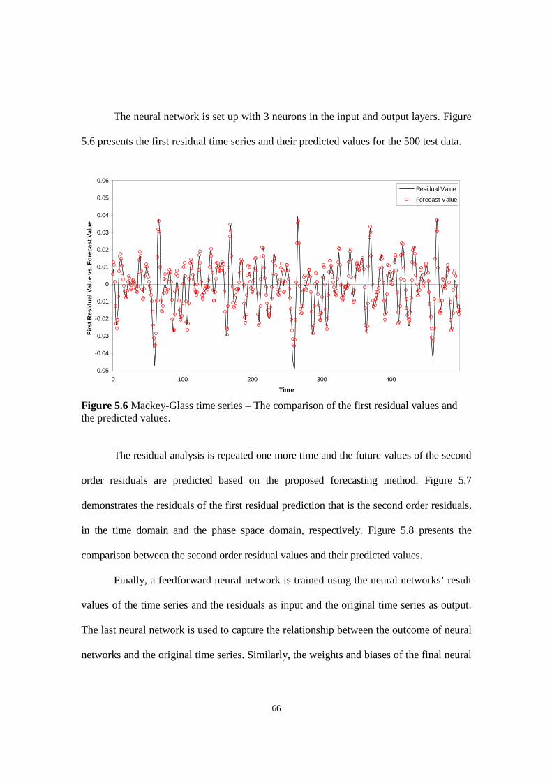
66

The neural network is set up with 3 neurons in the input and output layers. Figure

5.6 presents the first residual time series and their predicted values for the 500 test data.

-0.05

-0.04

-0.03

-0.02

-0.01

0

0.01

0.02

0.03

0.04

0.05

0.06

0 100 200 300 400

Time

Fir

st

Resid

ualV

alu

evs.F

ore

cast

Valu

e

Residual Value

Forecast Value

Figure 5.6 Mackey-Glass time series – The comparison of the first residual values andthe predicted values.

The residual analysis is repeated one more time and the future values of the second

order residuals are predicted based on the proposed forecasting method. Figure 5.7

demonstrates the residuals of the first residual prediction that is the second order residuals,

in the time domain and the phase space domain, respectively. Figure 5.8 presents the

comparison between the second order residual values and their predicted values.

Finally, a feedforward neural network is trained using the neural networks’ result

values of the time series and the residuals as input and the original time series as output.

The last neural network is used to capture the relationship between the outcome of neural

networks and the original time series. Similarly, the weights and biases of the final neural

67

network are improved using genetic algorithms and kept to predict the future value of

time series. Figure 5.9 compares the original values of the Mackey-Glass time series with

their predicted values.

Figure 5.7 Mackey-Glass time series – The second residual values, a) in time domain b)in phase space domain.

-0.01

0

0.01

0.02

0 100 200 300 400

Time

Seco

nd

Resid

ualV

alu

evs.F

ore

cast

Valu

e

Residual Value

Forecast Value

Figure 5.8 Mackey-Glass time series – The comparison of the second residual values andthe predicted values.

a) b)

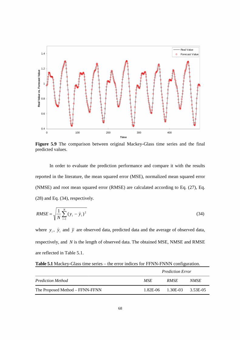
68

0.4

0.6

0.8

1

1.2

1.4

0 100 200 300 400

Time

RealV

alu

evs.F

ore

cast

Valu

e

Real Value

Forecast Value

Figure 5.9 The comparison between original Mackey-Glass time series and the finalpredicted values.

In order to evaluate the prediction performance and compare it with the results

reported in the literature, the mean squared error (MSE), normalized mean squared error

(NMSE) and root mean squared error (RMSE) are calculated according to Eq. (27), Eq.

(28) and Eq. (34), respectively.

N

iii yy

NRMSE

1

2)(1

(34)

where iy , iy

and y are observed data, predicted data and the average of observed data,

respectively, and N is the length of observed data. The obtained MSE, NMSE and RMSE

are reflected in Table 5.1.

Table 5.1 Mackey-Glass time series – the error indices for FFNN-FNNN configuration.

Prediction Error

Prediction Method MSE RMSE NMSE

The Proposed Method – FFNN-FFNN 1.82E-06 1.30E-03 3.53E-05

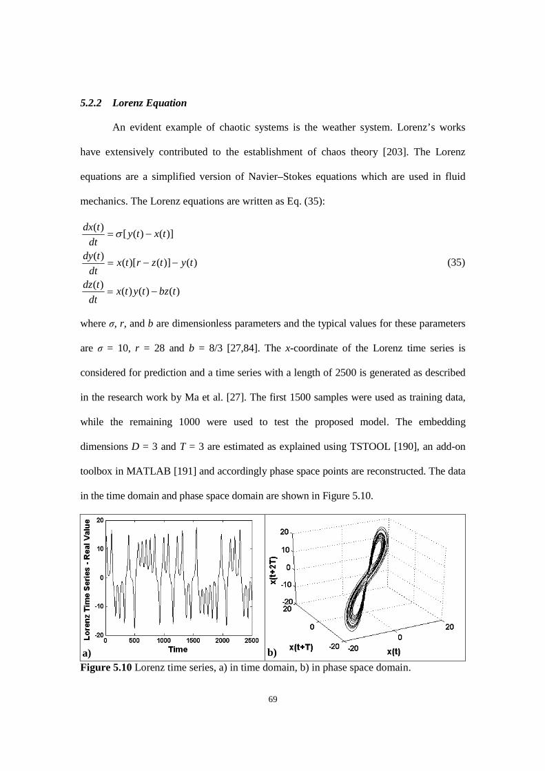
69

5.2.2 Lorenz Equation

An evident example of chaotic systems is the weather system. Lorenz’s works

have extensively contributed to the establishment of chaos theory [203]. The Lorenz

equations are a simplified version of Navier–Stokes equations which are used in fluid

mechanics. The Lorenz equations are written as Eq. (35):

)()()()(

)()]()[()(

)]()([)(

tbztytxdt

tdz

tytzrtxdt

tdy

txtydt

tdx

(35)

where σ, r, and b are dimensionless parameters and the typical values for these parameters

are σ = 10, r = 28 and b = 8/3 [27,84]. The x-coordinate of the Lorenz time series is

considered for prediction and a time series with a length of 2500 is generated as described

in the research work by Ma et al. [27]. The first 1500 samples were used as training data,

while the remaining 1000 were used to test the proposed model. The embedding

dimensions D = 3 and T = 3 are estimated as explained using TSTOOL [190], an add-on

toolbox in MATLAB [191] and accordingly phase space points are reconstructed. The data

in the time domain and phase space domain are shown in Figure 5.10.

Figure 5.10 Lorenz time series, a) in time domain, b) in phase space domain.

a) b)

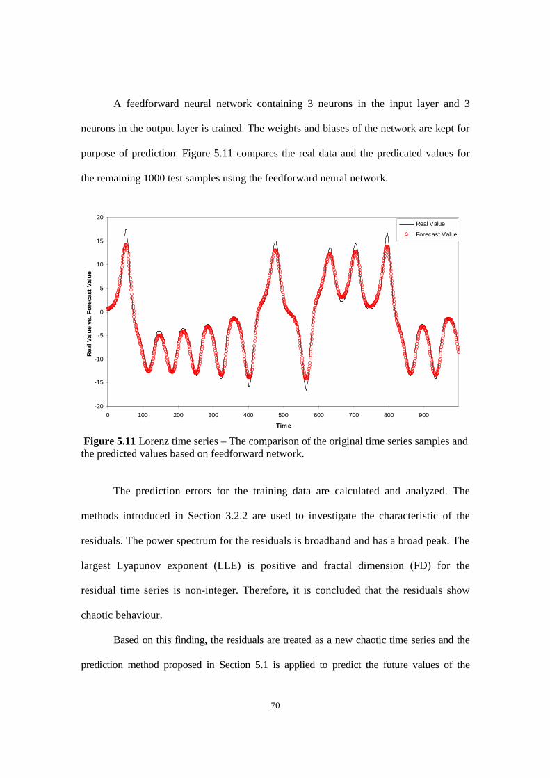
70

A feedforward neural network containing 3 neurons in the input layer and 3

neurons in the output layer is trained. The weights and biases of the network are kept for

purpose of prediction. Figure 5.11 compares the real data and the predicated values for

the remaining 1000 test samples using the feedforward neural network.

-20

-15

-10

-5

0

5

10

15

20

0 100 200 300 400 500 600 700 800 900

Time

RealV

alu

evs.F

ore

cast

Valu

e

Real Value

Forecast Value

Figure 5.11 Lorenz time series – The comparison of the original time series samples andthe predicted values based on feedforward network.

The prediction errors for the training data are calculated and analyzed. The

methods introduced in Section 3.2.2 are used to investigate the characteristic of the

residuals. The power spectrum for the residuals is broadband and has a broad peak. The

largest Lyapunov exponent (LLE) is positive and fractal dimension (FD) for the

residual time series is non-integer. Therefore, it is concluded that the residuals show

chaotic behaviour.

Based on this finding, the residuals are treated as a new chaotic time series and the

prediction method proposed in Section 5.1 is applied to predict the future values of the

71

residuals. The first (D-1)T+1 observations will help to predict the first prediction; therefore,

the length of residual time series is (D-1)T+1 shorter than the original time series. The

residuals may not inherit the same characteristics as the original time series; therefore, they

need to be analyzed independently. Therefore, 1493 samples are reconstructed with the new

embedding dimension D1 = 3 and time delay T1 = 3 for the residual time series. Figure 5.12

shows the first residual time series in the time domain and the phase space domain. Figure

5.13 presents the results of the first order residuals prediction.

The second level of residual analysis is performed and the evidence of chaos is

observed in the residuals. The second level of residuals are treated as a new time series

and predicted using a new feedforward neural network.

Figure 5.12 Lorenz time series – The first residuals a) in the time domain, b) in the phasespace domain.

Finally, a feedforward network is trained using the neural networks’ result values

of the time series and the residuals as input and the original time series as output to

a) b)

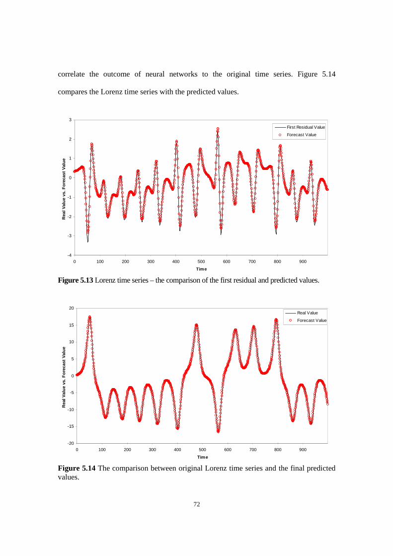
72

correlate the outcome of neural networks to the original time series. Figure 5.14

compares the Lorenz time series with the predicted values.

-4

-3

-2

-1

0

1

2

3

0 100 200 300 400 500 600 700 800 900

Time

Rea

lV

alu

evs.F

ore

cas

tV

alu

e

First Residual Value

Forecast Value

Figure 5.13 Lorenz time series – the comparison of the first residual and predicted values.

-20

-15

-10

-5

0

5

10

15

20

0 100 200 300 400 500 600 700 800 900

Time

RealV

alu

evs.F

ore

cast

Valu

e

Real Value

Forecast Value

Figure 5.14 The comparison between original Lorenz time series and the final predictedvalues.

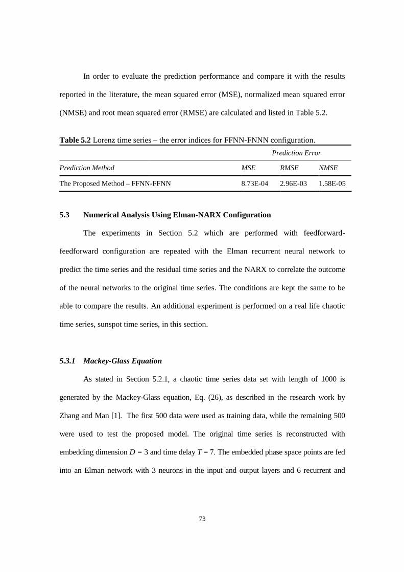
73


reported in the literature, the mean squared error (MSE), normalized mean squared error

(NMSE) and root mean squared error (RMSE) are calculated and listed in Table 5.2.

Table 5.2 Lorenz time series – the error indices for FFNN-FNNN configuration.

Prediction Error


The Proposed Method – FFNN-FFNN 8.73E-04 2.96E-03 1.58E-05

5.3 Numerical Analysis Using Elman-NARX Configuration

The experiments in Section 5.2 which are performed with feedforward-

feedforward configuration are repeated with the Elman recurrent neural network to

predict the time series and the residual time series and the NARX to correlate the outcome

of the neural networks to the original time series. The conditions are kept the same to be

able to compare the results. An additional experiment is performed on a real life chaotic

time series, sunspot time series, in this section.


As stated in Section 5.2.1, a chaotic time series data set with length of 1000 is

generated by the Mackey-Glass equation, Eq. (26), as described in the research work by

Zhang and Man [1]. The first 500 data were used as training data, while the remaining 500

were used to test the proposed model. The original time series is reconstructed with

embedding dimension D = 3 and time delay T = 7. The embedded phase space points are fed

into an Elman network with 3 neurons in the input and output layers and 6 recurrent and

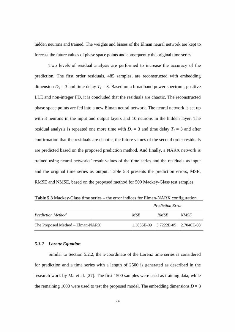
74

hidden neurons and trained. The weights and biases of the Elman neural network are kept to

forecast the future values of phase space points and consequently the original time series.

Two levels of residual analysis are performed to increase the accuracy of the

prediction. The first order residuals, 485 samples, are reconstructed with embedding

dimension D1 = 3 and time delay T1 = 3. Based on a broadband power spectrum, positive

LLE and non-integer FD, it is concluded that the residuals are chaotic. The reconstructed

phase space points are fed into a new Elman neural network. The neural network is set up

with 3 neurons in the input and output layers and 10 neurons in the hidden layer. The

residual analysis is repeated one more time with D2 = 3 and time delay T2 = 3 and after

confirmation that the residuals are chaotic, the future values of the second order residuals

are predicted based on the proposed prediction method. And finally, a NARX network is

trained using neural networks’ result values of the time series and the residuals as input

and the original time series as output. Table 5.3 presents the prediction errors, MSE,

RMSE and NMSE, based on the proposed method for 500 Mackey-Glass test samples.

Table 5.3 Mackey-Glass time series – the error indices for Elman-NARX configuration.

Prediction Error


The Proposed Method – Elman-NARX 1.3855E-09 3.7222E-05 2.7040E-08

5.3.2 Lorenz Equation

Similar to Section 5.2.2, the x-coordinate of the Lorenz time series is considered

for prediction and a time series with a length of 2500 is generated as described in the

research work by Ma et al. [27]. The first 1500 samples were used as training data, while

the remaining 1000 were used to test the proposed model. The embedding dimensions D = 3

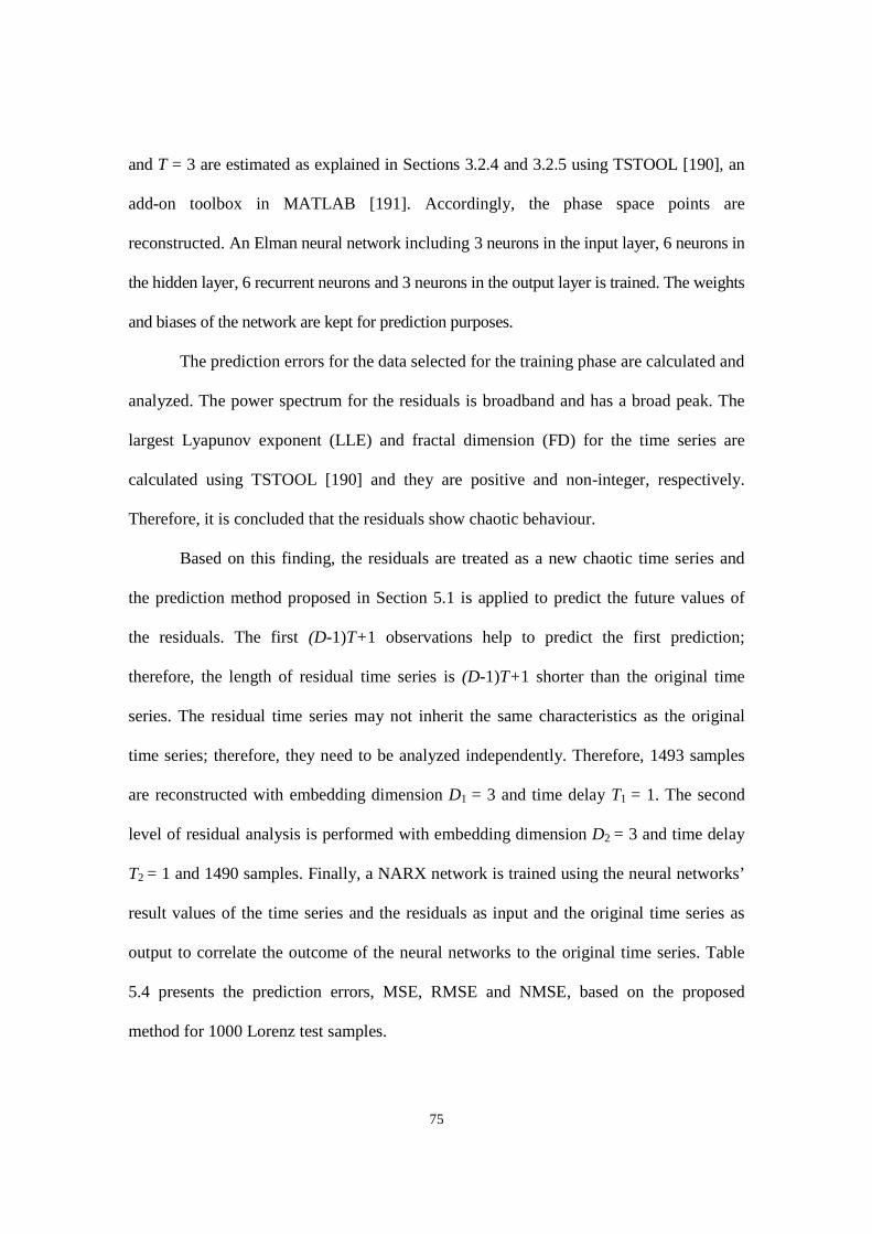
75

and T = 3 are estimated as explained in Sections 3.2.4 and 3.2.5 using TSTOOL [190], an

add-on toolbox in MATLAB [191]. Accordingly, the phase space points are

reconstructed. An Elman neural network including 3 neurons in the input layer, 6 neurons in

the hidden layer, 6 recurrent neurons and 3 neurons in the output layer is trained. The weights

and biases of the network are kept for prediction purposes.

The prediction errors for the data selected for the training phase are calculated and

analyzed. The power spectrum for the residuals is broadband and has a broad peak. The

largest Lyapunov exponent (LLE) and fractal dimension (FD) for the time series are

calculated using TSTOOL [190] and they are positive and non-integer, respectively.

Therefore, it is concluded that the residuals show chaotic behaviour.

Based on this finding, the residuals are treated as a new chaotic time series and

the prediction method proposed in Section 5.1 is applied to predict the future values of

the residuals. The first (D-1)T+1 observations help to predict the first prediction;

therefore, the length of residual time series is (D-1)T+1 shorter than the original time

series. The residual time series may not inherit the same characteristics as the original

time series; therefore, they need to be analyzed independently. Therefore, 1493 samples

are reconstructed with embedding dimension D1 = 3 and time delay T1 = 1. The second

level of residual analysis is performed with embedding dimension D2 = 3 and time delay

T2 = 1 and 1490 samples. Finally, a NARX network is trained using the neural networks’

result values of the time series and the residuals as input and the original time series as

output to correlate the outcome of the neural networks to the original time series. Table

5.4 presents the prediction errors, MSE, RMSE and NMSE, based on the proposed

method for 1000 Lorenz test samples.

76

Table 5.4 Lorenz time series – the error indices for Elman-NARX configuration.

Prediction Error



5.3.3 Sunspot Time Series

Forecasting solar activity is a challenging area and important topic for various

researchers and industries [82]. The sunspot time series is a good indication of solar

activity for solar cycles. The impact of solar activity has been observed on earth, climate,

weather, satellites and space missions; therefore, it is critical to forecast the sunspot time

series. However, because of the complexity of the system and the lack of a mathematical

model, forecasting the solar cycle is extremely challenging [84].

The monthly smoothed sunspot time series has been obtained from the SIDC

(World Data Center for the Sunspot Index) [204]. To compare the results with some of

the research works published in the literature, data are selected in the same conditions

reported by Ma et al. [27] and Gholipour et al. [84]. The sunspot series from November

1834 to June 2001 (2000 points) are selected and scaled between [0,1]. The first 1000

samples of time series are selected to train and the remaining 1000 samples are kept to test

the prediction method. The parameters D = 5 and T = 1 are estimated and accordingly the

phase space points are reconstructed. The Elman neural network consists of 5 neurons in

the input layer, 7 neurons in the hidden layer, 7 recurrent neurons and 5 neurons in the

output layer. The network is trained using a gradient descent with momentum and adaptive

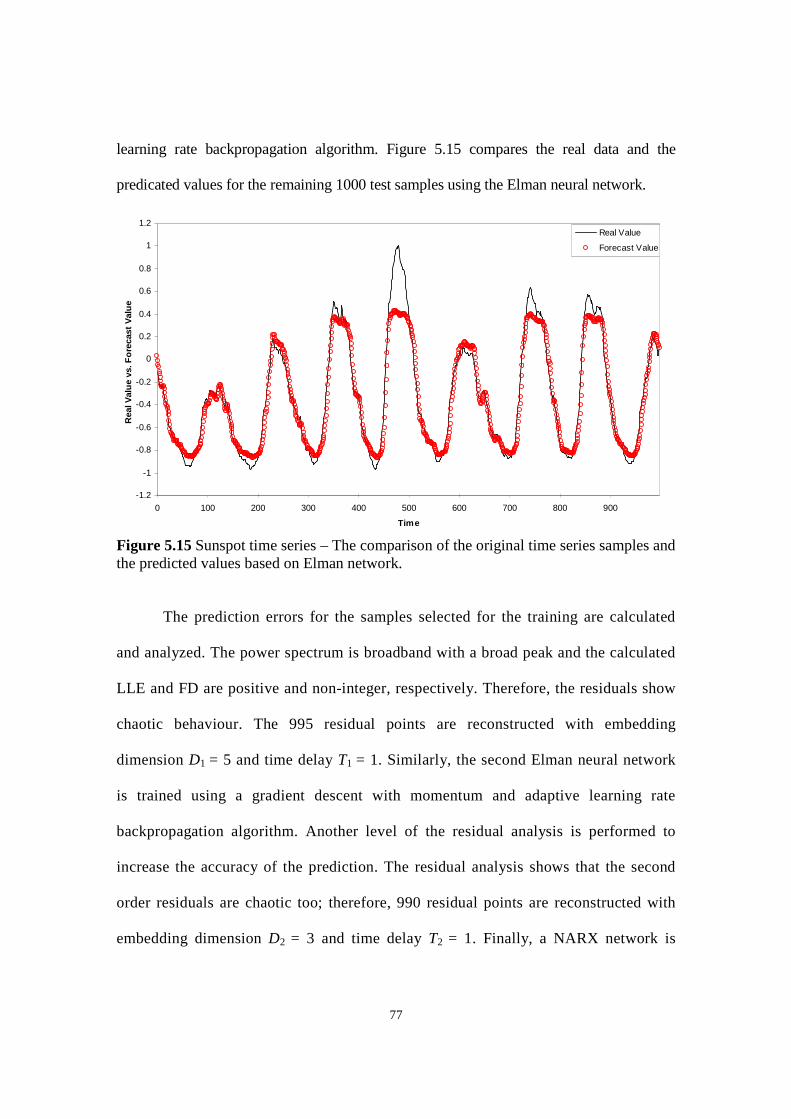
77

learning rate backpropagation algorithm. Figure 5.15 compares the real data and the

predicated values for the remaining 1000 test samples using the Elman neural network.

-1.2

-1

-0.8

-0.6

-0.4

-0.2

0

0.2

0.4

0.6

0.8

1

1.2

0 100 200 300 400 500 600 700 800 900

Time

RealV

alu

evs.F

ore

cast

Valu

e

Real Value

Forecast Value

Figure 5.15 Sunspot time series – The comparison of the original time series samples andthe predicted values based on Elman network.

The prediction errors for the samples selected for the training are calculated

and analyzed. The power spectrum is broadband with a broad peak and the calculated

LLE and FD are positive and non-integer, respectively. Therefore, the residuals show

chaotic behaviour. The 995 residual points are reconstructed with embedding

dimension D1 = 5 and time delay T1 = 1. Similarly, the second Elman neural network

is trained using a gradient descent with momentum and adaptive learning rate

backpropagation algorithm. Another level of the residual analysis is performed to

increase the accuracy of the prediction. The residual analysis shows that the second

order residuals are chaotic too; therefore, 990 residual points are reconstructed with

embedding dimension D2 = 3 and time delay T2 = 1. Finally, a NARX network is

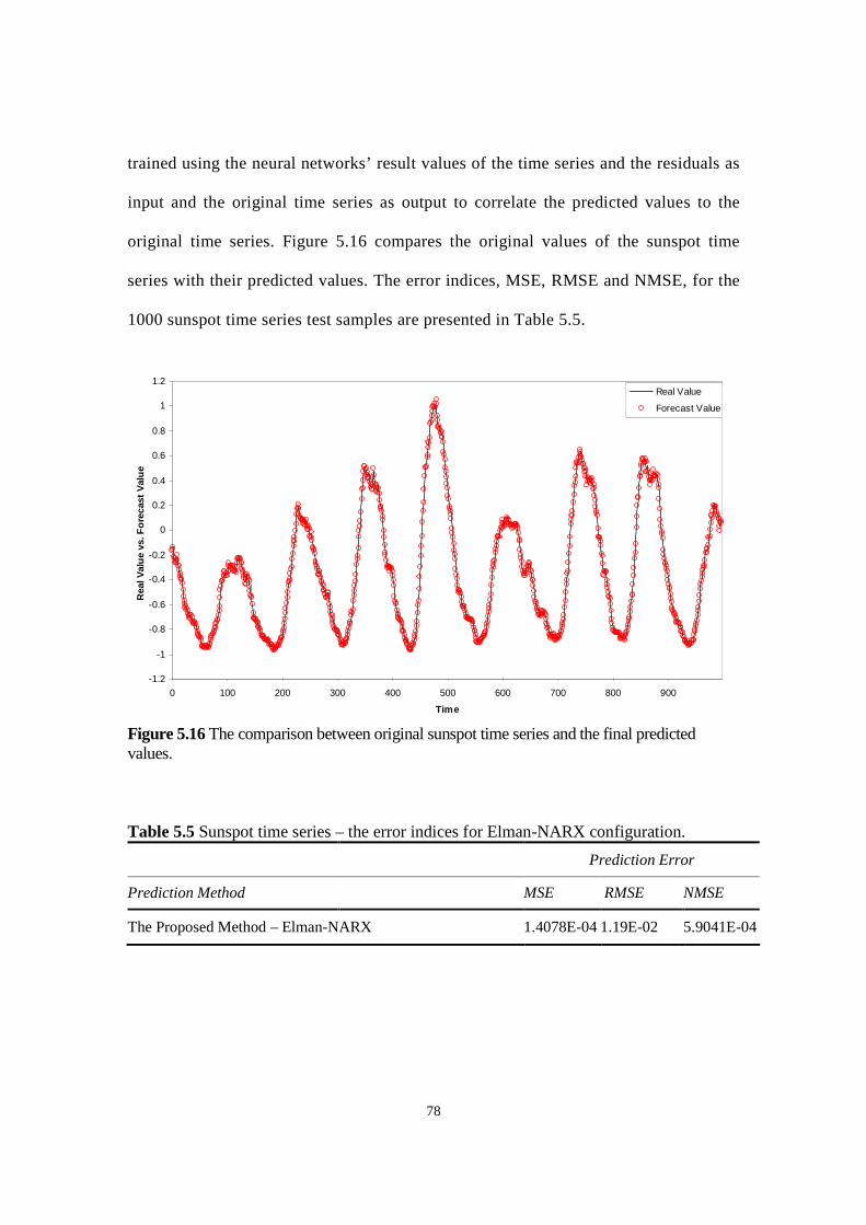
78

trained using the neural networks’ result values of the time series and the residuals as

input and the original time series as output to correlate the predicted values to the

original time series. Figure 5.16 compares the original values of the sunspot time

series with their predicted values. The error indices, MSE, RMSE and NMSE, for the

1000 sunspot time series test samples are presented in Table 5.5.

-1.2

-1

-0.8

-0.6

-0.4

-0.2

0

0.2

0.4

0.6

0.8

1

1.2

0 100 200 300 400 500 600 700 800 900

Time

RealV

alu

evs.F

ore

cast

Valu

e

Real Value

Forecast Value

Figure 5.16 The comparison between original sunspot time series and the final predictedvalues.

Table 5.5 Sunspot time series – the error indices for Elman-NARX configuration.

Prediction Error



79


To evaluate the proposed forecasting methods both in feedforward and Elman-

NARX configurations, the prediction accuracy of the methods when applied to the

Mackey-Glass, Lorenz and sunspot time series as benchmarking are compared to the

prediction performance of the methods presented in the literature.

For the Mackey-Glass time series, the performance of the proposed method in this

chapter is compared with the results reported in the literature. Wang and Mendel [205]

developed a forecasting method which generates fuzzy rules from sample data. In the

paper published by Cho and Wang [115], a method based on a neuro-fuzzy system with

adaptive capability to extract fuzzy if-then rules from input and output numerical data

through learning is suggested. The method by Cho and Wang [115] which is called radial

basis function (RBF) based adaptive fuzzy system (AFS) used Gaussian functions as the

membership functions of the premise portion of fuzzy rules. Also, Jang et al. [145] and

Zhang et al. [39] used neuro-fuzzy method to forecast chaotic time series.

In the research work by Rojas et al. [116], a framework to configure and train a

radial basis function (RBF) is introduced. A sequential learning algorithm is adopted to

organize the structure of the network. Pseudo-Gaussian function (PG) is used to modify

the structure of the Gaussian functions. Rojas et al. [31] developed an expert system

based on artificial intelligence in which the parameters of the ARMA model could be

determined automatically. In this study, a hybrid forecasting method was introduced

based on the artificial neural network and ARMA.

Kim and Kim [154] proposed a genetic fuzzy predictor ensemble (GFPE) method

to predict the future of chaotic time series. Gholipour et al. [84] examined several neural

80

and neuro-fuzzy models with different learning algorithms for prediction of several

benchmark chaotic time series. The performance of locally linear neuro-fuzzy models

with the developed locally linear model tree (LoLiMoT) learning algorithm is compared

with the prediction performance of radial basis function (RBF) neural network with

orthogonal least squares (OLS) learning algorithm, multi-layer perceptron neural network

with error backpropagation learning algorithm, and adaptive network based fuzzy

inference system.

Teo et al. [122] used a wavelet packet multi-layer perceptron neural network

(WP-MLP) trained by backpropagation learning method for prediction of chaotic time

series. Zhang and Man [1] developed a multi-dimension chaotic time series prediction

method using recurrent neural network (RNN) in embedding phase space. Similarly,

Assaad et al. [107] proposed a forecasting method based on boosted recurrent neural

networks. Inoue et al. [206] used hybrid neural networks to forecast chaotic time series.

Table 5.6 presents the comparison between the prediction errors, MSE, RMSE

and NMSE, reported in the literature and the proposed method for 500 Mackey-Glass test

samples. The results in Table 5.6 are sorted based on RMSE error index. Although

ERNN method shows close results compared to the proposed method for Mackey-Glass

time series, in other benchmarking time series the proposed forecasting method

supersedes ERNN method. The results show that the proposed forecasting method with

Elman-NARX configuration performs better in prediction of the Mackey-Glass chaotic

time series when compared to other prediction methods reported in the literature.

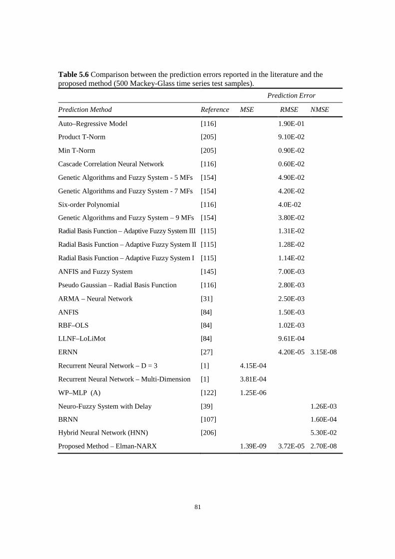
81

Table 5.6 Comparison between the prediction errors reported in the literature and theproposed method (500 Mackey-Glass time series test samples).

Prediction Error

Prediction Method Reference MSE RMSE NMSE

Auto–Regressive Model [116] 1.90E-01

Product T-Norm [205] 9.10E-02

Min T-Norm [205] 0.90E-02

Cascade Correlation Neural Network [116] 0.60E-02

Genetic Algorithms and Fuzzy System - 5 MFs [154] 4.90E-02

Genetic Algorithms and Fuzzy System - 7 MFs [154] 4.20E-02

Six-order Polynomial [116] 4.0E-02

Genetic Algorithms and Fuzzy System – 9 MFs [154] 3.80E-02

Radial Basis Function – Adaptive Fuzzy System III [115] 1.31E-02

Radial Basis Function – Adaptive Fuzzy System II [115] 1.28E-02

Radial Basis Function – Adaptive Fuzzy System I [115] 1.14E-02

ANFIS and Fuzzy System [145] 7.00E-03

Pseudo Gaussian – Radial Basis Function [116] 2.80E-03

ARMA – Neural Network [31] 2.50E-03

ANFIS [84] 1.50E-03

RBF–OLS [84] 1.02E-03

LLNF–LoLiMot [84] 9.61E-04

ERNN [27] 4.20E-05 3.15E-08

Recurrent Neural Network – D = 3 [1] 4.15E-04

Recurrent Neural Network – Multi-Dimension [1] 3.81E-04

WP–MLP (A) [122] 1.25E-06

Neuro-Fuzzy System with Delay [39] 1.26E-03

BRNN [107] 1.60E-04

Hybrid Neural Network (HNN) [206] 5.30E-02

Proposed Method – Elman-NARX 1.39E-09 3.72E-05 2.70E-08

82

The prediction performance for the Lorenz time series based on the proposed

method in this chapter is compared with the same of the forecasting methods presented in

the research works in the literature. The performance of the forecasting methods by Jang

et al. [145], Rojas et al. [116], Rojas et al. [31], Gholipour et al. [84], Ma et al. [27] and

Assaad et al. [107] when applied to the Lorenz time series is listed in Table 5.7.

Iokibe et al. [207] used local fuzzy reconstruction method in short-term prediction

of chaotic time series. Martinez-Rego et al. [22] used local dynamic modeling to develop

a new forecasting method to predict chaotic time series. The suggested method by

Martinez-Rego et al. [22] is consisted of three element of time delay line; information

theoretic based clustering method and a set of single layer neural networks. Tao and Xiao

[30] and Dhahri and Alimi [208] used a radial basis function network and Garcia and

Alarcon [40] employed wavelet networks to forecast chaotic time series.

The prediction accuracy for the 1000 Lorenz time series test samples, for the

demonstrated experiments based on feedforward-feedforward configuration and Elamn-

NARX configuration are compared with the results reported in the literature. Table 5.7

presents the comparison between the prediction errors, MSE, RMSE and NMSE

reported in the literature and the proposed method for 1000 Lorenz test samples. These

experiments confirm that the proposed method with Elman-NARX, when it is used to

forecast the future values of the Lorenz time series, generates better results compared to

other prediction methods reported in the literature.

83

Table 5.7 Comparison between the prediction errors reported in the literature and theproposed method (1000 Lorenz time series test samples).

Prediction Error


Local Fuzzy Reconstruction [207] 2.44E-01

Adaptive Neuro-Fuzzy Inference Systems (ANFIS) [145] 1.43E-01



Support Vector Regression [22] 1.46E-02

TDL-MLP [22] 1.56E-04

DLE-VQIT [22] 2.58E-04

RBF with Orthogonal LS [84] 1.41E-09

LLNF-LoLiMot [84] 9.80E-10

CIFCA-ROLSA [30] 1.30E-03

ROLSA [30] 4.63E-02

Evolving Recurrent Neural Network (ERNN) [27] 9.90E-10

Boosted Recurrent Neural Networks (BRNN) [107] 3.77E-03

MDE-RBF [208] 1.70E-01

Wavelet-Networks B [40] 1.64E-02

Proposed Method – Elman-NARX -- 1.173E-08 1.083E-04 1.983E-10

The performance of the proposed forecasting method in this chapter when applied

to the sunspot time series is compared with the results published by Sello [82], Gholipour

et al. [84], Teo et al. [122], McNish and Lincoln [209], Denkmayr and Cugnon [210], Ma

et al. [27] and Koskela et al. [127].

The forecasting method proposed by Sello [82] is based on a local hypothesis of

the behaviour on embedding space, employing an optimal number of neighbouring

vectors to forecast the future projection. Koskela et al. [127] has compared the

84

performance of a multi-layer neural network, finite impulse response (FIR) and an Elman

neural network when applied to the sunspot time series prediction.

The error indices, MSE, RMSE and NMSE for the 1000 sunspot time series test

samples are compared with the results reported in the literature and presented in Table 5.8.

The experiment performed for the sunspot time series confirms that the performance of

the proposed method with Elman-NARX configuration is better in prediction of the

sunspot time series when compared to other prediction methods reported in the literature.

Table 5.8 Comparison between the prediction errors reported in the literature and theproposed method (1000 sunspot time series test samples).

Prediction Error


Denkmayr [210] 1.85

Waldmeier [82] 5.60E-01

Sello – Nonlinear Method [82] 3.40E-01

WP-MLP (A) [122] 1.25E-01

Multi-Layer Perceptron (MLP) [127] 9.79E-02

McNish-Lincoln [209] 8.00E-02

RBF-OLS [84] 4.60E-02


ERNN [27] 1.29E-02 2.80E-03

Proposed Method – Elman-NARX -- 1.41E-04 1.19E-02 5.90E-04

5.5 Summary

In this chapter, a new prediction method was developed using a combination of the

embedding theorem, residual analysis, ensemble neural networks and genetic algorithms to

predict chaotic time series. Based on the embedding theorem, the original time series can

85

be unfolded with the embedding dimension and time delay and reconstructed into the phase

space points. A neural network was used to predict the future values of the embedded phase

space points. In some cases, the residuals of the forecasting method are not random and

follow the characteristics of the original time series. The accuracy of the prediction method

was further enhanced by analyzing and incorporating the residuals. The residual analysis

was repeated several times. Eventually, to capture the relationship between the outcome of

neural networks and the original time series, a new neural network was trained. Two

configurations for the ensemble neural networks were implemented. In the first

configuration, all the selected neural networks were feedforward neural networks. In the

second configuration, the combination of Elman and NARX neural networks was utilized.

The developed methods with both feedforward-feedforward and Elman-NARX

configurations have been validated for a one-step ahead prediction. The performance of the

proposed forecasting methods in terms of error indices has been compared with the

performance of reported forecasting methods in the literature. In the current chapter, the

neural network architectures and their parameters are determined arbitrarily. In the next

chapter, Taguchi’s DOE will be implemented to select proper neural network architectures

and parameters and improve the performance of the proposed forecasting method.

Despite its simplicity in implementation, the proposed model exhibited a superior

performance in predicting the chaotic time series. The developed algorithm was applied

to two chaotic systems, Mackey-Glass and Lorenz equations and a real life sunspot time

series. It has been concluded that the proposed model can perform more effectively and

accurately as compared to other prediction methods for chaotic time series.

86

CHAPTER 6

TAGUCHI’S DESIGN OF EXPERIMENTS INCOMBINATION SELECTION FOR CHAOTIC TIMESERIES FORECASTING METHOD USINGENSEMBLE ARTIFICIAL NEURAL NETWORKS

Taguchi’s design of experiments is an efficient approach to identify the proper factor-

level combinations utilized to improve the result of the proposed forecasting method for

chaotic time series. In the proposed method, residual analysis using a combination of

embedding theorem and ensemble artificial neural networks is utilized to forecast chaotic

time series. Based on the embedding theorem, the embedding parameters are determined

and the time series is reconstructed into proper phase space points. The embedded phase

space points are fed into the first neural network and trained. The weights and biases are

kept to predict the future values of the phase space points and the chaotic time series. The

residual of the predicted time series is analyzed, and it was observed that in some events

the residuals demonstrate chaotic behaviour. The residuals are considered as a new

chaotic time series and reconstructed according to the embedding theorem. A new neural

network is trained to predict the future values of the residual time series. The residual

analysis can be repeated several times. Finally, the last neural network is trained using the

neural networks’ result values of the time series and the residuals as input and the

original time series as output. The final network is used to capture the relationship

87

between the neural networks’ result values and the original time series. A systematic

approach is introduced using Taguchi’s design of experiments to select proper

combinations of ensemble artificial neural networks and their parameters.

The method is applied to the Mackey-Glass and the Lorenz equations which produce

chaotic time series, and two real life chaotic time series, sunspot and far-infrared NH3 laser

time series, to evaluate the performance of the proposed technique. The experimental results

confirm that the proposed method can predict the chaotic time series more effectively and

accurately when compared with the same method using arbitrary selection of architectures

and parameters and other existing forecasting methods in the literature.

The content of the current chapter has been presented at the International

Conference on Industrial Engineering and Systems Management [211] and submitted to

the journal of Neural Computing and Applications [212].

6.1 Introduction to Taguchi’s Design of Experiments

In the applications where multiple variables are involved, it is essential to

determine the best solution by identifying the proper levels of the variables. Design of

experiments (DOE) is a practical tool to investigate the impact on the outcome of a

system while changing the variables and to determine the appropriate levels.

The idea of DOE was first introduced by Sir Ronald Fisher in the early 1920s

when he proposed a systematic and analytical method to determine the impact of multiple

factors on the output of his experiments [213,214]. Factorial experimental design in

which experiments are carried out for all factor-level combinations was used by Fisher.

88

Taguchi in 1949 developed a method which utilized orthogonal arrays (OA) to

reduce the experimental numbers while maintaining reasonably sufficient information

[45,47,50,215,216]. Taguchi’s method gained its reputation mainly in the early 1980s

[217]. Taguchi’s DOE is usually performed with the aid of an analysis of variance

(ANOVA). It is one of the most effective techniques for improving the performance of a

system by selecting the optimum levels for the involved parameters.

DOE has been utilized by many practitioners for optimization and modelling

purposes. The contribution of Taguchi’s method to DOE is to simplify the use of this

method. This simplification has expanded the applications of DOE.

Many applications of Taguchi’s DOE are reported in the literature. Among

them, Wang et al. [218] has adopted Taguchi’s method to optimize the experimental

conditions for the gas chromatographic-mass spectrometric determination. Taguchi

method is used by Naidu and Gowda [219] in spray-painting application and Gandhi

[220] in the gear sub-assembly of gearboxes. Manna and Bhattacharyya [221] used

Taguchi’s method to optimize wire EDM parameters for aluminum reinforced metal

matrix composite. Taguchi’s DOE has helped Sukthomya and Tannock [222] to

develop an important manufacturing process for aircraft engines, Mezgar et al. [223] to

develop a robust manufacturing system and Tsai and Mort [224] to optimize an

integrated manufacturing system.

Taguchi’s method has been adopted by many researchers in the field of artificial

neural networks (ANN) to find an optimum design for the networks. Kim and Yum

[43], Khaw et al. [44], Lin and Tseng [45], Ortiz-Rodríguez et al. [46], Packianather

and Drake [47], Wang et al. [48], Yang and Lee [49] and Peterson et al. [50] have used

89

Taguchi’s DOE to optimize the design of ANN. Mouli et al. [51] has demonstrated that

Taguchi’s method can be utilized as a pre-step to the neural network method to obtain

the optimum result.

In the current research work, Taguchi’s design of experiments is utilized as a prior

step to determine the factor-level combinations to improve the performance of the

proposed method to forecast chaotic time series.

6.2 Taguchi’s Design of Experiments Method

Taguchi’s design of experiments is an efficient method to identify the optimum

factor-level combinations to minimize variation while maintaining the mean at the desired

level. Taguchi’s DOE can improve the performance of a process or a system with a limited

number of experimental data based on orthogonal arrays (OA). OA is the matrix of

combinations with the shortest possible elements. Similar to DOE, the purpose of

Taguchi’s method is to study the impact on the performance of the system while all the

design parameters are simultaneously varied. The two important elements in selecting the

orthogonal arrays are the factors and interactions and the levels for each factor [51].

The standard orthogonal arrays established by Taguchi contain 18 basic OA. The

name of the OA indicates the number of rows, columns and the number of levels in each

column. For instance, orthogonal array L27(310) consists of 27 rows and 10 columns and

each column has 3 levels. When an appropriate OA is selected, a table of combinations

will be formed and the experiments will be performed for each row of the OA table. The

results of the experiments will be analyzed using the analysis of variance (ANOVA)

method. Based on Taguchi’s approach, the ratio of signal (target or the mean of the

90

outcomes) to the noise (square deviation of the outcomes) which is called the S/N ratio

can be calculated by Eq. (36):

n iznNS

210

11log10/ (36)

where n is the number of variables and zi is the value of each variable. For each level of

each parameter, the S/N ratios are calculated and the graphs are generated. The proper

level for each parameter is achieved based on the highest S/N ratio [51].

6.2 Implementation of Taguchi’s DOE to the Forecasting Method

The process of forecasting the future values of a time series using residual

analysis and the ensemble method involves a number of parameters including the neural

network architecture, the neural network transfer function, the training method and

others, which affect the end result. In this study, Taguchi’s design of experiments is

employed to improve the proposed forecasting method by selecting the factors and their

levels, positioning them appropriately into a suitable OA, and conducting experiments.

The factors are selected from neural network architectures: FFNN, Elman and NARX,

MATLAB [191] transfer functions: purelin and tansig and MATLAB [191] training

methods: traingdx, trainbr and trainlm. Weights and biases of the neural networks which

cause variation in the result of the forecasting method are considered as noise factors.

Each experiment is taken from the OA and the performance of the forecasting method is

measured for that trial. The performance of the forecasting method is determined by the

normalized mean square error (NMSE) of the real data and the forecast values. The

resulting performances for all the experiments are analyzed and the appropriate

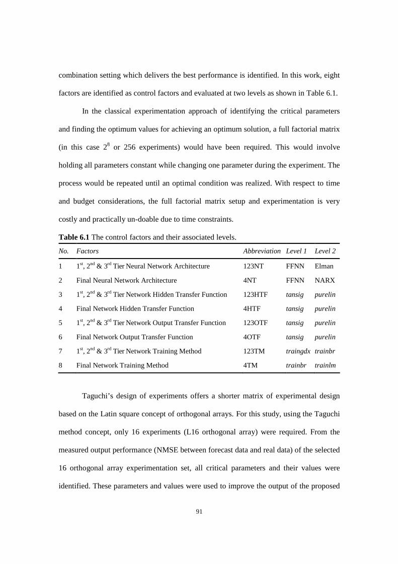
91

combination setting which delivers the best performance is identified. In this work, eight

factors are identified as control factors and evaluated at two levels as shown in Table 6.1.

In the classical experimentation approach of identifying the critical parameters

and finding the optimum values for achieving an optimum solution, a full factorial matrix

(in this case 28 or 256 experiments) would have been required. This would involve

holding all parameters constant while changing one parameter during the experiment. The

process would be repeated until an optimal condition was realized. With respect to time

and budget considerations, the full factorial matrix setup and experimentation is very

costly and practically un-doable due to time constraints.

Table 6.1 The control factors and their associated levels.

No. Factors Abbreviation Level 1 Level 2

1 1st, 2nd & 3rd Tier Neural Network Architecture 123NT FFNN Elman

2 Final Neural Network Architecture 4NT FFNN NARX

3 1st, 2nd & 3rd Tier Network Hidden Transfer Function 123HTF tansig purelin

4 Final Network Hidden Transfer Function 4HTF tansig purelin

5 1st, 2nd & 3rd Tier Network Output Transfer Function 123OTF tansig purelin

6 Final Network Output Transfer Function 4OTF tansig purelin

7 1st, 2nd & 3rd Tier Network Training Method 123TM traingdx trainbr

8 Final Network Training Method 4TM trainbr trainlm

Taguchi’s design of experiments offers a shorter matrix of experimental design

based on the Latin square concept of orthogonal arrays. For this study, using the Taguchi

method concept, only 16 experiments (L16 orthogonal array) were required. From the

measured output performance (NMSE between forecast data and real data) of the selected

16 orthogonal array experimentation set, all critical parameters and their values were

identified. These parameters and values were used to improve the output of the proposed

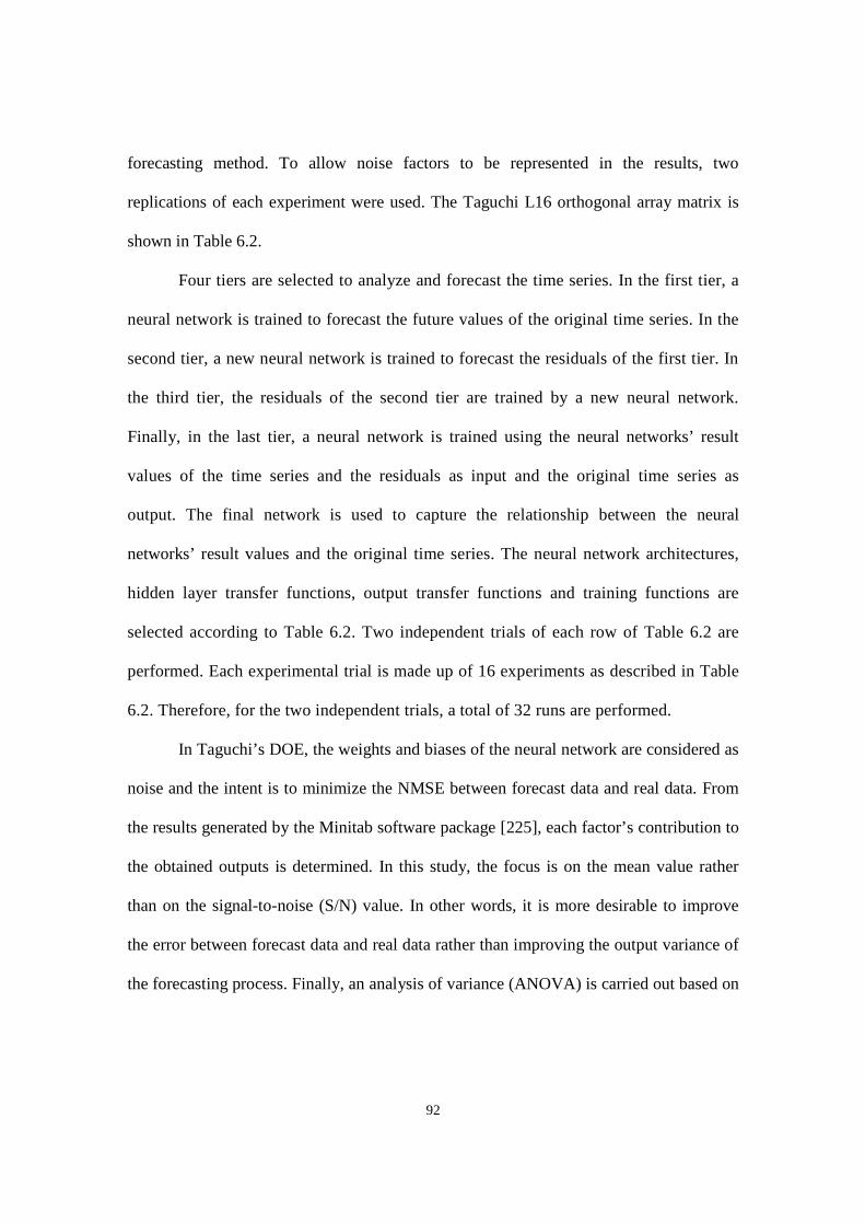
92

forecasting method. To allow noise factors to be represented in the results, two

replications of each experiment were used. The Taguchi L16 orthogonal array matrix is

shown in Table 6.2.

Four tiers are selected to analyze and forecast the time series. In the first tier, a

neural network is trained to forecast the future values of the original time series. In the

second tier, a new neural network is trained to forecast the residuals of the first tier. In

the third tier, the residuals of the second tier are trained by a new neural network.

Finally, in the last tier, a neural network is trained using the neural networks’ result

values of the time series and the residuals as input and the original time series as

output. The final network is used to capture the relationship between the neural

networks’ result values and the original time series. The neural network architectures,

hidden layer transfer functions, output transfer functions and training functions are

selected according to Table 6.2. Two independent trials of each row of Table 6.2 are

performed. Each experimental trial is made up of 16 experiments as described in Table

6.2. Therefore, for the two independent trials, a total of 32 runs are performed.

In Taguchi’s DOE, the weights and biases of the neural network are considered as

noise and the intent is to minimize the NMSE between forecast data and real data. From

the results generated by the Minitab software package [225], each factor’s contribution to

the obtained outputs is determined. In this study, the focus is on the mean value rather

than on the signal-to-noise (S/N) value. In other words, it is more desirable to improve

the error between forecast data and real data rather than improving the output variance of

the forecasting process. Finally, an analysis of variance (ANOVA) is carried out based on

93

the prepared experiments and their output results. A confidence level of 95 percent was

selected to evaluate the importance of each factor.

Table 6.2 Taguchi’s DOE setting; orthogonal array L16 (28).

No. 123NT 4NT 123HTF 4HTF 123OTF 4OTF 123TM 4TM

1 FF FF tansig tansig tansig tansig traingdx trainbr

2 FF FF tansig purelin tansig purelin trainbr trainlm

3 FF FF purelin tansig purelin tansig trainbr trainlm

4 FF FF purelin purelin purelin purelin traingdx trainbr

5 FF NARX tansig tansig purelin purelin traingdx trainlm

6 FF NARX tansig purelin purelin tansig trainbr trainbr

7 FF NARX purelin tansig tansig purelin trainbr trainbr

8 FF NARX purelin purelin tansig tansig traingdx trainlm

9 Elman FF tansig tansig purelin purelin trainbr trainbr

10 Elman FF tansig purelin purelin tansig traingdx trainlm

11 Elman FF purelin tansig tansig purelin traingdx trainlm

12 Elman FF purelin purelin tansig tansig trainbr trainbr

13 Elman NARX tansig tansig tansig tansig trainbr trainlm

14 Elman NARX tansig purelin tansig purelin traingdx trainbr

15 Elman NARX purelin tansig purelin tansig traingdx trainbr

16 Elman NARX purelin purelin purelin purelin trainbr trainlm

6.3 Numerical Analysis Using Taguchi’s DOE Method

In order to evaluate the proposed method, the developed technique is applied to two

chaotic systems, Mackey-Glass and Lorenz equations and two real life chaotic time series,

sunspot and far-infrared time series. Later, the performance of the forecasting method

configured by the appropriate factor-level combinations determined by Taguchi’s design of

94

experiment is compared with the results of the same forecasting method with arbitrary

selection of architectures and parameters and the results reported in the literature.

6.3.1 Lorenz Equations

The details of the Lorenz equations have been presented in Section 5.2.2. Similar

to Section 5.2.2 the parameters in Eq. (35) are selected according to the previous reports

[27,84]. The x-coordinate of the Lorenz time series is considered for prediction and a time

series with a length of 2500 is generated as described in the research work by Ma et al.

[27]. The first 1500 samples were used as training data, while the remaining 1000 were

used to test the proposed model.


The details of the Mackey-Glass equation have been presented in Section 4.2.1.

Similar to Section 4.2.1, the parameters in Eq. (26) are selected according to the previous

report by Zhang et al. [66], where the constants are taken to be a = 0.2, b = 0.1 and c = l0

and chaotic time series is generated by τ =17 and initial value x(0) = 1.2. A chaotic time

series data set with length of 1000 is generated by Eq. (26). The first 500 data were used

as training data, while the remaining 500 were used to test the proposed model.

6.3.3 Sunspot Time Series

The details of the sunspot time series have been presented in Section 5.3.3. The

monthly smoothed sunspot time series has been obtained from the SIDC (World Data

Center for the Sunspot Index) [204]. To compare the results with some of the studies

95

published in the literature, data are selected in the same conditions reported by Ma et al.

[27] and Gholipour et al. [84]. The sunspot series from November 1834 to June 2001

(2000 points) are selected and scaled between [0,1]. The first 1000 samples of the time

series are selected for training and the remaining 1000 samples are kept to test the

prediction method.

6.3.4 Far-Infrared NH3 Laser Time Series

The far-infrared NH3 Laser time series is set A from the Santa Fe time series

forecasting competition [226,227]. It is a real world data set recorded from the far-

infrared NH3 laser in a chaotic state. The training set is a series of 1000 values and the

goal is to apply the proposed forecasting method in this study to forecast one step ahead

for the next 100 data.

6.3.5 Numerical Experiments

The embedding parameters for the Lorenz time series D = 3 and T = 3, the

Mackey-Glass time series D = 3 and T = 7, the sunspot time series D = 5 and T = 1 and

the far-infrared NH3 laser time series D = 7 and T = 2 are estimated using TSTOOL

[190] and accordingly phase space points are reconstructed.

For all the time series, the embedding dimensions (D1 & D2) and time delays (T1

& T2) for the second and third tiers are selected based on the characteristics of the

residuals. The neural network architectures and the remaining parameters are selected

according to Table 6.2. Table 6.3 presents the performance of the forecasting method

(NMSE) for each experiment for all four time series.

96

Table 6.3 Taguchi’s DOE setting; orthogonal array L16(28).

Lorenz Mackey-Glass Sunspot NH3 Laser

No. RUN1 RUN2 RUN1 RUN2 RUN1 RUN2 RUN1 RUN2

1 2.9549 2.9502 2.8145 2.8223 1.6482 1.6487 8.27E-01 8.28E-01

2 2.7552 2.7551 2.9158 2.916 1.6578 1.6612 8.05E-01 8.05E-01

3 2.853 2.848 2.9606 2.9608 1.6323 1.6321 8.15E-01 8.14E-01

4 2.953 2.9533 2.7606 2.7704 1.6242 1.6243 8.25E-01 8.25E-01

5 3.00E-05 3.00E-05 8.80E-04 8.79E-04 3.89E-04 3.84E-04 8.04E-02 8.03E-02

6 9.55E-01 9.56E-01 3.38E-01 3.38E-01 7.10E-01 7.09E-01 5.81E-01 5.82E-01

7 8.13E-01 8.13E-01 4.22E-01 4.28E-01 9.03E-02 9.11E-02 5.03E-01 5.04E-01

8 6.30E-05 6.29E-05 4.22E-05 4.21E-05 6.03E-03 6.03E-03 6.03E-02 6.03E-02

9 2.01643 2.01642 2.6813 2.6797 1.6094 1.6091 8.20E-01 8.19E-01

10 7.11E-01 7.12E-01 1.91116 1.91217 1.0056 1.0043 3.20E-01 3.21E-01

11 6.64E-01 6.55E-01 1.98107 1.9811 1.1314 1.1317 4.88E-01 4.87E-01

12 2.2823 2.2832 2.5983 2.5982 1.5314 1.5316 8.88E-01 8.86E-01

13 2.31E-09 2.30E-09 4.37E-06 4.29E-06 2.55E-03 2.56E-03 9.26E-03 9.28E-03

14 3.20E-09 3.22E-09 5.72E-05 5.73E-05 5.63E-04 5.60E-04 7.73E-03 7.69E-03

15 3.31E-08 3.31E-08 9.2E-06 9.21E-06 5.60E-05 5.61E-05 4.30E-02 4.31E-02

16 1.20E-10 1.19E-10 5.62E-07 5.62E-07 5.59E-04 5.59E-04 8.30E-03 8.32E-03

The results of the ANOVA at 95% confidence level are shown in Table 6.4. Each

column in Table 6.4 contains information regarding the determination of the significance

of each factor to the response (NMSE). The factor with the largest F value has the

greatest impact and based on that, the ranking of each factor is determined as shown in

the response Table 6.5 [225]. For all four time series, the F Test at 95% level of

confidence indicated that Tier Neural Network Architecture, Final Neural Network

97

Architecture, Tier Network Training Method and Final Network Training Method among

other factors are significant because their p-values are less than 0.05.

Table 6.4 The result of ANOVA analysis.

Lorenz Mackey-Glass Sunspot NH3 Laser

Factors F P F P F P F P

123NT 20.48 0.003 19.63 0.003 11.86 0.011 58.66 0.000

4NT 84 0.000 831.52 0.000 330.32 0.000 322.93 0.000

123HTF 0.01 0.923 0.01 0.927 1.04 0.342 0.51 0.500

4HTF 0.05 0.834 0.24 0.64 0.48 0.51 0.13 0.730

123OTF 0.0000 0.989 0.01 0.909 0.71 0.428 0.14 0.715

4OTF 0.11 0.751 0.04 0.843 0.48 0.513 0.000 0.979

123TM 6.83 0.035 12.55 0.009 8.99 0.020 50.51 0.000

4TM 8.83 0.021 7.25 0.031 8.57 0.022 58.31 0.000

The response Table 6.5 shows the average of each response for each level of each

factor. The table of responses determines the rank of each factor based on Delta statistics,

which compares the relative magnitude of effects. The ranks are assigned according to

the Delta values with the highest Delta value being the first rank [225]. Therefore, based

on the response Table 6.5, Final Neural Network Architecture and Tier Neural Network

Architecture have the greatest influence for all four time series. The Tier Network

Training Method and the Final Network Training Method have the next influence for the

Mackey-Glass and sunspot time series, respectively, and with the change in the order;

Final Network Training and Tier Network Training have the next influence for the

Lorenz and far-infrared NH3 laser time series, respectively.

98

Table 6.5 The response table for Lorenz time series, Mackey-Glass time series, sunspot

time series and far-infrared NH3 laser time series.

Time Series Level 123NT 4NT 123HTF 4HTF 123OTF 4OTF 123TM 4TM

1 0.7088 2.1478 1.1949 1.2073 1.1859 1.1497 1.4592 1.4967

2 1.66 0.2211 1.174 1.1616 1.1829 1.2192 0.9097 0.8722

Delta 0.9512 1.9266 0.021 0.0458 0.003 0.0694 0.5496 0.6246Lorenz

Rank 2 1 7 6 8 5 4 3

1 1.14645 2.579 1.34132 1.31618 1.33216 1.34612 1.48979 1.45321

2 1.52805 0.0955 1.33318 1.35832 1.34234 1.32838 1.1847 1.22128

Delta 0.38161 2.4835 0.00815 0.04215 0.01019 0.01773 0.30509 0.23193Mackey-Glass

Rank 2 1 8 5 7 6 3 4

1 0.6601 1.4802 0.7521 0.8171 0.8226 0.7646 0.9045 0.9018

2 0.9214 0.1013 0.8294 0.7644 0.7589 0.8169 0.677 0.6797

Delta 0.2613 1.3789 0.0773 0.0527 0.0638 0.0523 0.2274 0.2221Sunspot

Rank 2 1 5 7 6 8 3 4

1 0.3229 0.7233 0.4536 0.4369 0.4366 0.4421 0.5536 0.5618

2 0.5622 0.1617 0.4314 0.4481 0.4485 0.443 0.3315 0.3232

Delta 0.2394 0.5616 0.0222 0.0112 0.0119 0.0008 0.2221 0.2386NH3 Laser

Rank 2 1 5 7 6 8 4 3


The purpose of this study is to improve the performance of the developed forecasting

method by reducing NMSE; therefore, the factor-levels which produce the lowest mean are

desirable. The level averages in the response Table 6.5 show that the means are minimized

when the Tier Neural Network Architecture is Elman, Final Neural Network Architecture is

NARX, the Tier Network Training Method is traingdx and the Final Network Training

Method is trainlm. The remaining factors do not show any significance.

99

The proper levels which are obtained from Taguchi’s DOE are used in the

prediction of the four selected time series. In order to evaluate the forecasting

performance and compare this with the results reported in the literature, the mean

squared error (MSE), normalized mean squared error (NMSE) and root mean squared

error (RMSE) are calculated.

The prediction accuracy of the proposed method when the parameters are selected

arbitrarily or with Taguchi’s DOE is compared to the prediction performance of the

methods presented in the literature for the Lorenz time series. The performance of the

forecasting methods by Jang et al. [145], Rojas et al. [116], Rojas et al. [31], Gholipour et

al. [84], Ma et al. [27] and Assaad et al. [107], Iokibe et al. [207], Martinez-Rego et al.

[22], Tao and Xiao [30], Dhahri and Alimi [208] and Garcia and Alarcon [40] when

applied to the Lorenz time series is listed in Table 6.6. Figure 6.1 compares the original

values of the Lorenz time series with their predicted values.

-20

-15

-10

-5

0

5

10

15

20

0 100 200 300 400 500 600 700 800 900

Time

RealV

alu

evs.F

ore

cast

Valu

e

Real Value

Forecast Value


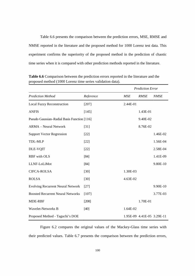
100

Table 6.6 presents the comparison between the prediction errors, MSE, RMSE and

NMSE reported in the literature and the proposed method for 1000 Lorenz test data. This

experiment confirms the superiority of the proposed method in the prediction of chaotic

time series when it is compared with other prediction methods reported in the literature.

Table 6.6 Comparison between the prediction errors reported in the literature and the

proposed method (1000 Lorenz time series validation data).

Prediction Error


Local Fuzzy Reconstruction [207] 2.44E-01

ANFIS [145] 1.43E-01

Pseudo Gaussian–Radial Basis Function [116] 9.40E-02


Support Vector Regression [22] 1.46E-02

TDL-MLP [22] 1.56E-04

DLE-VQIT [22] 2.58E-04

RBF with OLS [84] 1.41E-09


CIFCA-ROLSA [30] 1.30E-03

ROLSA [30] 4.63E-02

Evolving Recurrent Neural Network [27] 9.90E-10

Boosted Recurrent Neural Networks [107] 3.77E-03

MDE-RBF [208] 1.70E-01

Wavelet-Networks B [40] 1.64E-02

Proposed Method - Taguchi’s DOE 1.95E-09 4.41E-05 3.29E-11

Figure 6.2 compares the original values of the Mackey-Glass time series with

their predicted values. Table 6.7 presents the comparison between the prediction errors,

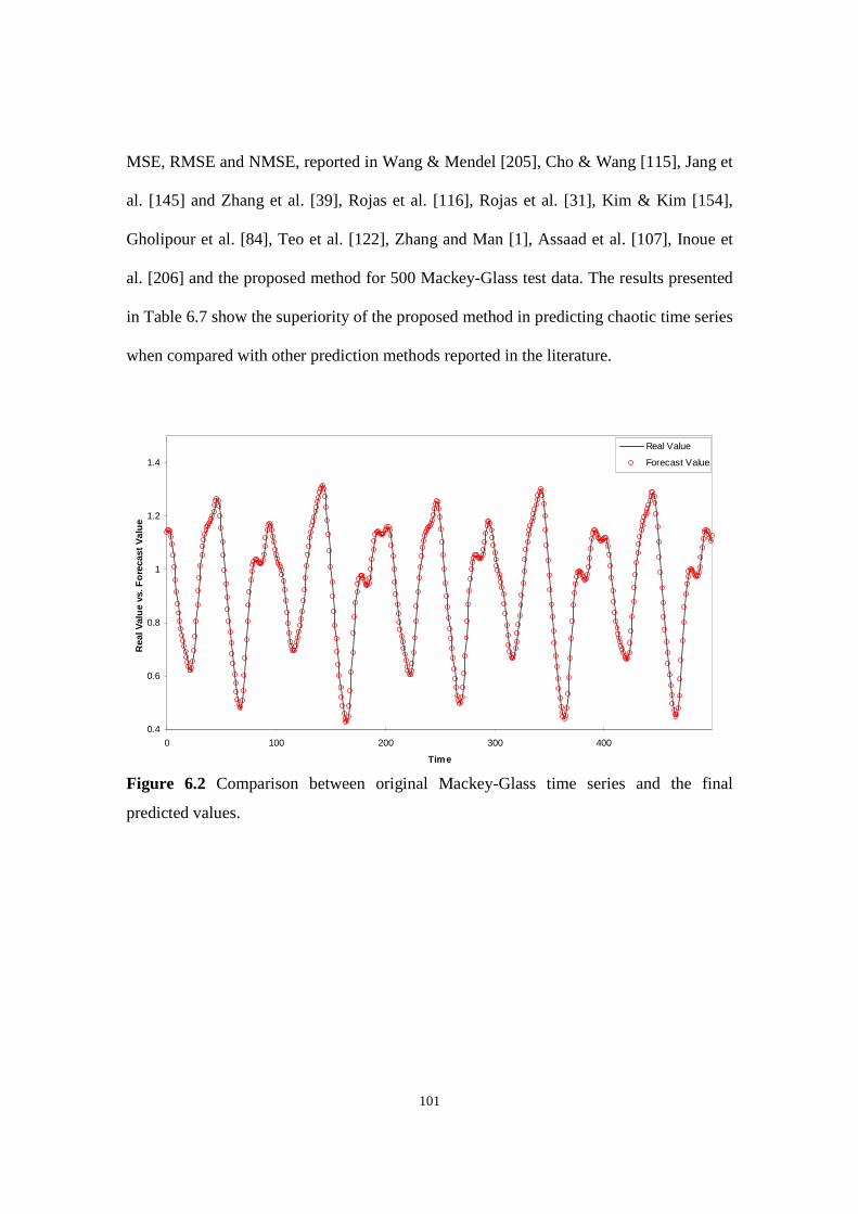
101

MSE, RMSE and NMSE, reported in Wang & Mendel [205], Cho & Wang [115], Jang et

al. [145] and Zhang et al. [39], Rojas et al. [116], Rojas et al. [31], Kim & Kim [154],

Gholipour et al. [84], Teo et al. [122], Zhang and Man [1], Assaad et al. [107], Inoue et

al. [206] and the proposed method for 500 Mackey-Glass test data. The results presented

in Table 6.7 show the superiority of the proposed method in predicting chaotic time series

when compared with other prediction methods reported in the literature.

0.4

0.6

0.8

1

1.2

1.4

0 100 200 300 400

Time

RealV

alu

evs.F

ore

cast

Valu

e

Real Value

Forecast Value

Figure 6.2 Comparison between original Mackey-Glass time series and the final

predicted values.

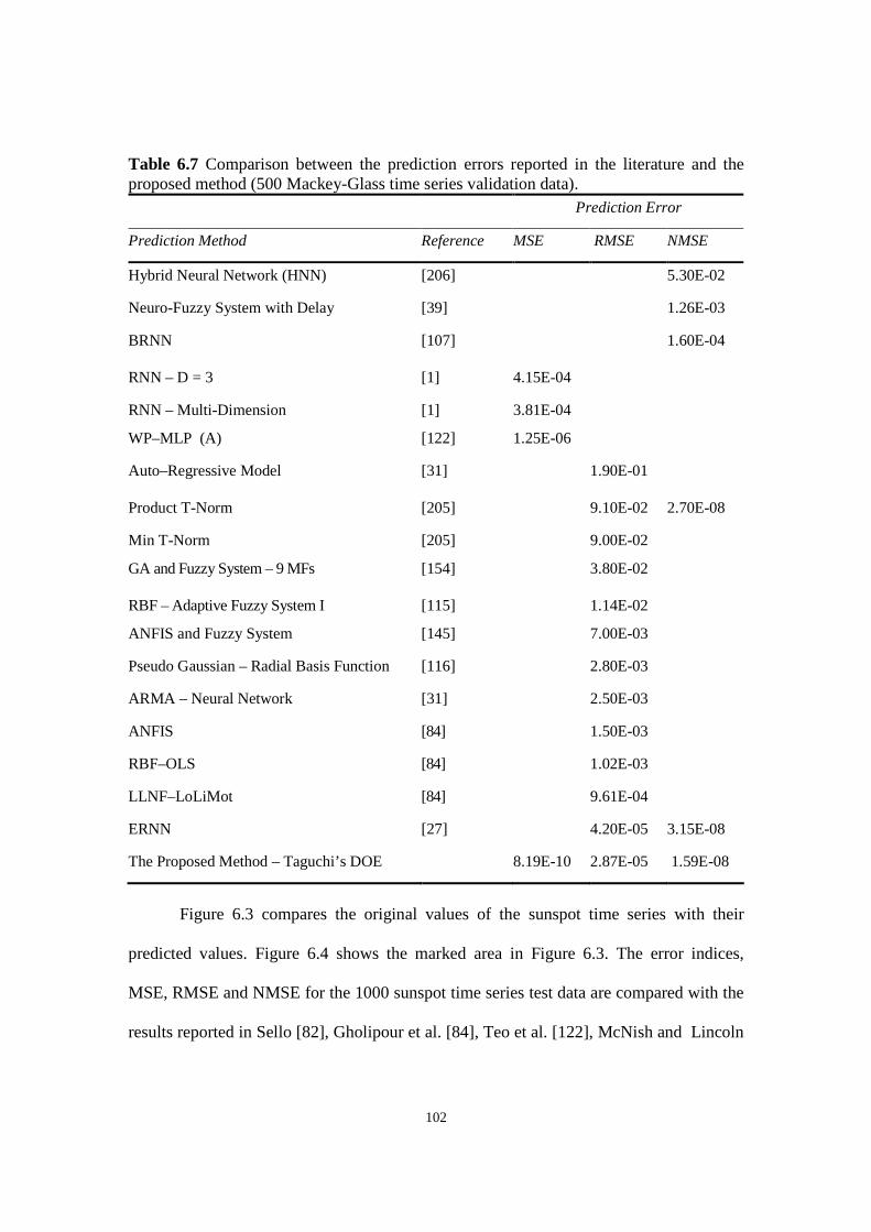
102

Table 6.7 Comparison between the prediction errors reported in the literature and theproposed method (500 Mackey-Glass time series validation data).

Prediction Error


Hybrid Neural Network (HNN) [206] 5.30E-02

Neuro-Fuzzy System with Delay [39] 1.26E-03

BRNN [107] 1.60E-04

RNN – D = 3 [1] 4.15E-04

RNN – Multi-Dimension [1] 3.81E-04

WP–MLP (A) [122] 1.25E-06

Auto–Regressive Model [31] 1.90E-01

Product T-Norm [205] 9.10E-02 2.70E-08

Min T-Norm [205] 9.00E-02

GA and Fuzzy System – 9 MFs [154] 3.80E-02

RBF – Adaptive Fuzzy System I [115] 1.14E-02

ANFIS and Fuzzy System [145] 7.00E-03



ANFIS [84] 1.50E-03

RBF–OLS [84] 1.02E-03

LLNF–LoLiMot [84] 9.61E-04

ERNN [27] 4.20E-05 3.15E-08

The Proposed Method – Taguchi’s DOE 8.19E-10 2.87E-05 1.59E-08

Figure 6.3 compares the original values of the sunspot time series with their

predicted values. Figure 6.4 shows the marked area in Figure 6.3. The error indices,

MSE, RMSE and NMSE for the 1000 sunspot time series test data are compared with the

results reported in Sello [82], Gholipour et al. [84], Teo et al. [122], McNish and Lincoln

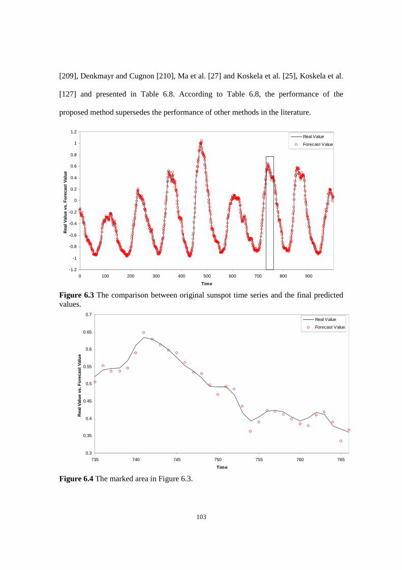
103

[209], Denkmayr and Cugnon [210], Ma et al. [27] and Koskela et al. [25], Koskela et al.

[127] and presented in Table 6.8. According to Table 6.8, the performance of the

proposed method supersedes the performance of other methods in the literature.

-1.2

-1

-0.8

-0.6

-0.4

-0.2

0

0.2

0.4

0.6

0.8

1

1.2

0 100 200 300 400 500 600 700 800 900

Time

RealV

alu

evs.F

ore

cast

Valu

e

Real Value

Forecast Value

Figure 6.3 The comparison between original sunspot time series and the final predictedvalues.

0.3

0.35

0.4

0.45

0.5

0.55

0.6

0.65

0.7

735 740 745 750 755 760 765

Time

RealV

alu

evs.F

ore

cast

Valu

e

Real Value

Forecast Value

Figure 6.4 The marked area in Figure 6.3.

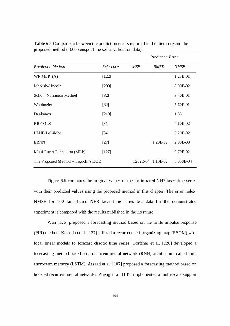
104


proposed method (1000 sunspot time series validation data).

Prediction Error


WP-MLP (A) [122] 1.25E-01

McNish-Lincoln [209] 8.00E-02

Sello – Nonlinear Method [82] 3.40E-01

Waldmeier [82] 5.60E-01

Denkmayr [210] 1.85

RBF-OLS [84] 4.60E-02


ERNN [27] 1.29E-02 2.80E-03

Multi-Layer Perceptron (MLP) [127] 9.79E-02

The Proposed Method – Taguchi’s DOE 1.202E-04 1.10E-02 5.038E-04

Figure 6.5 compares the original values of the far-infrared NH3 laser time series

with their predicted values using the proposed method in this chapter. The error index,

NMSE for 100 far-infrared NH3 laser time series test data for the demonstrated

experiment is compared with the results published in the literature.

Wan [126] proposed a forecasting method based on the finite impulse response

(FIR) method. Koskela et al. [127] utilized a recurrent self-organizing map (RSOM) with

local linear models to forecast chaotic time series. Dorffner et al. [228] developed a

forecasting method based on a recurrent neural network (RNN) architecture called long

short-term memory (LSTM). Assaad et al. [107] proposed a forecasting method based on

boosted recurrent neural networks. Zheng et al. [137] implemented a multi-scale support

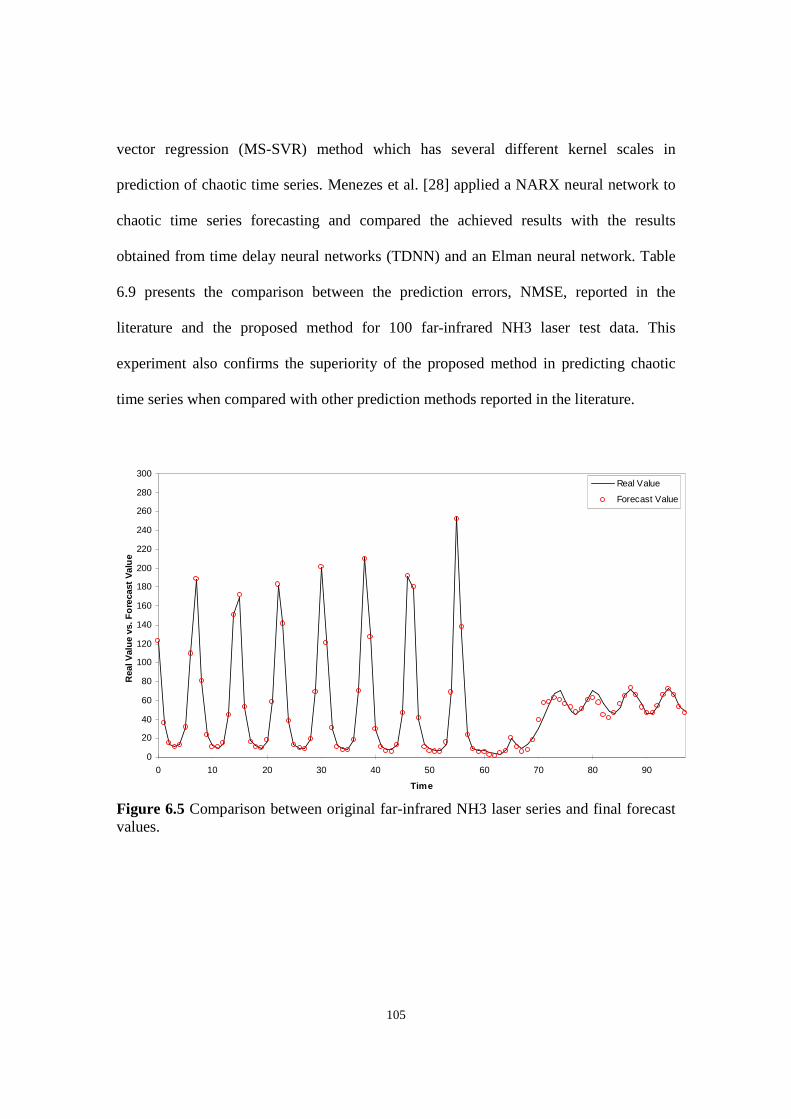
105

vector regression (MS-SVR) method which has several different kernel scales in

prediction of chaotic time series. Menezes et al. [28] applied a NARX neural network to

chaotic time series forecasting and compared the achieved results with the results

obtained from time delay neural networks (TDNN) and an Elman neural network. Table

6.9 presents the comparison between the prediction errors, NMSE, reported in the

literature and the proposed method for 100 far-infrared NH3 laser test data. This

experiment also confirms the superiority of the proposed method in predicting chaotic

time series when compared with other prediction methods reported in the literature.

0

20

40

60

80

100

120

140

160

180

200

220

240

260

280

300

0 10 20 30 40 50 60 70 80 90

Time

RealV

alu

evs.

Fo

recast

Va

lue

Real Value

Forecast Value

Figure 6.5 Comparison between original far-infrared NH3 laser series and final forecastvalues.

106


proposed method (100 far-infrared NH3 laser time series validation data).

Prediction Error Improvement

Prediction Method Reference NMSE Percentage

MLP [28] 1.72E-0198.1

MLP [228] 9.96E-0296.7

RSOM [127] 8.33E-0296.1

SVR [137] 5.80E-0294.4

LSTM [228] 3.96E-0291.8

MS-SVR [137] 3.92E-0291.7

LSTM IT [228] 3.64E-0291.1

Elman [28] 3.40E-0290.5

NARX [28] 3.39E-0290.4

FIR-MLP [126] 2.30E-0285.9

Weigend and Nix [229] 1.98E-0283.6

MLP [127] 1.78E-0281.8

MLP IT [228] 1.58E-0279.5

BPTT [107] 7.92E-0359.1

CBPTT [107] 5.60E-0342.1

EBPTT [107] 5.37E-0339.7

Boosting-Squared [107] 4.31E-0324.8

Boosting-Linear [107] 3.77E-0314.1

The Proposed Method – Taguchi’s DOE 3.24E-03

6.5 Summary

In this study, Taguchi’s design of experiments was utilized to identify the factor-

level combinations which improve the performance of the proposed method to forecast

chaotic time series. Based on the embedding theorem, the original time series can be

107

unfolded with embedding dimension and time delay and reconstructed into the phase space

points. The first neural network was trained, and the future values of the embedded phase

space points and, consequently, the original time series were predicted. It was observed

that, in some cases, the residuals of the forecasting method were not random and exhibited

the same characteristics as the original time series. The accuracy of this prediction method

was further enhanced by analyzing and incorporating the prediction residuals. The residual

analysis was repeated several times. Eventually, to capture the relationship between the

predicted values and the original time series, a new neural network was trained. Taguchi’s

design of experiments was introduced as a pre-step to the forecasting method to select

proper combinations of ensemble artificial neural networks and their parameters.

The performance of the improved forecasting method has been validated for a

one-step ahead prediction in terms of error indices. The results were compared with the

performance of reported forecasting methods in the literature. Two systems which

produce chaotic time series, Mackey-Glass and Lorenz, and two real life chaotic time

series, sunspot and a far-infrared NH3 laser time series, were selected for benchmarking.

In all four time series analysis, Tier Neural Network Architecture, Final Neural Network

Architecture, Tier Network Training Method and Final Network Training Method

showed importance and their selected levels were Elman, NARX, traingdx and trainlm,

respectively. The experimental results confirm that the selected levels identified by

Taguchi’s DOE have improved the performance of the proposed forecasting method

when compared with the same method using arbitrary selection of architectures and

parameters or other existing forecasting methods in the literature.

108

CHAPTER 7

APPLICATIONS OF CHAOTIC TIME SERIESFORECASTING

Applications of chaos theory are becoming increasingly widespread in a variety of

disciplines. Chaos theory has been applied to the control of robot servos [4]. The

implication of chaos has been observed in communications, the optimization of

telephone exchanges [5] and the transmission of digital signals [6]. Data analysis

methods developed for the analysis of chaotic behaviour have been applied to bulk

chemical reactions [7]. Chaos theory has also been applied to economics [230,231],

ecology [232], international relations [233] and medicine [234]. In the supply chain

management area, the principles of chaos theory have been used in demand forecasting,

product design and inventory management [19,235,236].

González and Pereda [17] utilized chaos theory to study the short-term

cardiovascular control system. Wichard et al. [237] applied chaos theory to the

balancing problem of spinning rotors. In the hydrological field, Jayawardena and Lai

[71] detected chaotic behaviour in daily rainfall and streamflow data. Feichtinger [238]

has discussed the importance of chaos theory in operations research. In the financial

sector, chaos theory has been applied mainly to commodity markets, stock markets,

exchange rates, bankruptcy prediction and financial planning [8].

109

Prediction of nonlinear and chaotic time series is a useful method to evaluate

characteristics of dynamical systems. Predictions of chaotic time series have been observed

in the areas of marketing [9,239], foreign exchange rates [10,102], signal processing [11],

supply chain management [12,19], oil price and consumption [240], traffic flow [13,241],

power load [14,242], weather forecasting [15], tidal prediction [72], sunspot prediction

[16], air quality [243], production systems [237] and many others. Due to the importance of

these fields, the interest in a robust technique to predict chaotic time series has increased.

In Chapter 6, the final form of the proposed forecasting method was presented.

This original forecasting method was developed using the embedding theorem,

ensemble neural networks, residual analysis, genetic algorithms and Taguchi’s design

of experiments. In the current chapter, the proposed method is applied to financial

markets, namely, stock markets and exchange rate trading. In the following sections,

the daily price of four stocks, namely, British Airlines, Southwest Airlines, Ryanair

Holdings and Lucent Incorporated, and two exchange rates, namely, EUR/USD and

USD/JPY, are analyzed and their future values are predicted.

7.1 Stock Markets

In the last few decades, stock markets have become an inseparable part of the

global economy. Any change in stock markets impacts on the financial status of

individuals, corporations and countries [244,245]. The crash of stock markets on October

19, 1987, increased the interests of macroeconomists and financial researchers to

investigate chaotic behaviour in stock markets. They observed that the large movements

110

in stock markets are greater than the expected normal distribution. Later, financial

economists concluded that stock markets are governed by chaotic dynamics [246].

The relationship between chaos theory and stock markets has been discussed

repeatedly in the literature [239,246,247,248]. In the financial sector, chaos theory has

been applied mainly to commodity markets, stock markets, exchange rates, bankruptcy

prediction, financial planning [8] and employment rates [239]. The research work by

Baumol and Benhabib [230] presents a comprehensive survey of economic models

which deal with chaotic behaviour of stock markets [246].

Forecasting the future of stock markets is a challenging and attractive subject

[9]. Stock markets are evolutionary, nonlinear and complex systems [249]. Numerous

factors are involved in prediction of stock markets including traders’ expectations,

general economic conditions and political events [139,250]. There is always some

degree of risk in investing in stock markets due to the difficulties in prediction of the

stock market movements [245]. Therefore, an appropriate forecasting model could

decrease the risk of such investments.

Saad et al. [251] utilized time delay neural networks (TDNN), recurrent neural

networks (RNN) and probabilistic neural networks (PNN) to forecast Apple stock

trends. Huanga et al. [250] investigated the predictability of financial movement

direction with a support vector machine (SVM) and applied the method to the weekly

movement direction of NIKKEI 225 stock data. Hassan and Nath [245] utilized a

hidden Markov model (HMM) approach to forecast stock prices for some airline stocks:

Southwest Airlines, British Airlines, Delta Airlines and Ryanair Holdings Ltd. Qian and

Rasheed [9] used the Hurst exponent to determine a period with great predictability for

111

the Dow Jones Industrial Average index. Afolabi and Olude [139] used

backpropagation, a Kohonen self-organizing map (SOM), and a hybrid Kohonen SOM

to forecast the daily price of Lucent Incorporated stock.

In this section, the proposed forecasting method using chaos theory, the embedding

theorem, residual analysis and improved ensemble neural networks with genetic algorithms

and Taguchi’s design of experiments is applied to the daily price of four stocks: British

Airlines, Southwest Airlines, Ryanair Holdings Ltd. and Lucent Incorporated.

7.1.1 British Airlines Stock Data

The daily price of British Airlines stock has been selected for analysis and

forecasting. In order to compare the performance of the proposed forecasting method in

this study when applied to British Airlines stock data with the results reported in the

literature, the conditions are set based on Hassan and Nath [245]. The daily stock data of

British Airlines for the period January 1, 2003 to September 10, 2004 which includes 443

data is selected for training of the developed model in this study. Accordingly, the daily

stock data for the period September 11, 2004 to January 10, 2005 which includes 94 data

is selected for testing of the proposed method to forecast one step ahead for the closing

price of British Airlines stock. Figure 7.1 shows the daily closing price of British Airlines

stock for the period January 1, 2003 to January 10, 2005.

The first step in applying the proposed forecasting method to British Airlines stock

data is to detect chaos in the time series. The Lyapunov exponent is the most popular

method to investigate the existence of chaos in a given time series [10,252,253,254]. A

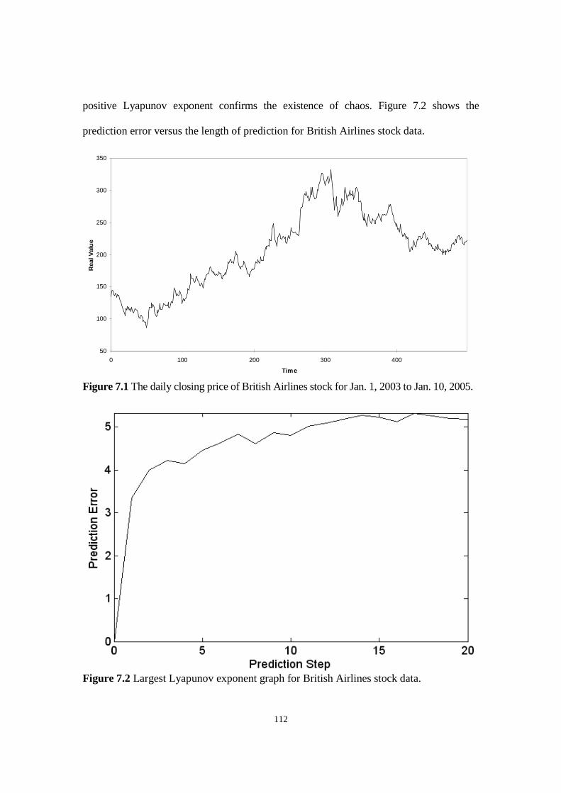
112

positive Lyapunov exponent confirms the existence of chaos. Figure 7.2 shows the

prediction error versus the length of prediction for British Airlines stock data.

50

100

150

200

250

300

350

0 100 200 300 400

Time

RealV

alu

e

Figure 7.1 The daily closing price of British Airlines stock for Jan. 1, 2003 to Jan. 10, 2005.

Figure 7.2 Largest Lyapunov exponent graph for British Airlines stock data.

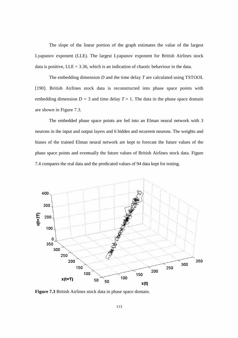
113

The slope of the linear portion of the graph estimates the value of the largest

Lyapunov exponent (LLE). The largest Lyapunov exponent for British Airlines stock

data is positive, LLE = 3.36, which is an indication of chaotic behaviour in the data.

The embedding dimension D and the time delay T are calculated using TSTOOL

[190]. British Airlines stock data is reconstructed into phase space points with

embedding dimension D = 3 and time delay T = 1. The data in the phase space domain

are shown in Figure 7.3.

The embedded phase space points are fed into an Elman neural network with 3

neurons in the input and output layers and 6 hidden and recurrent neurons. The weights and

biases of the trained Elman neural network are kept to forecast the future values of the

phase space points and eventually the future values of British Airlines stock data. Figure

7.4 compares the real data and the predicated values of 94 data kept for testing.

Figure 7.3 British Airlines stock data in phase space domain.

114

150

170

190

210

230

250

270

290

0

Time

RealV

alu

evs.F

ore

cast

Valu

e

Real Value

Forecast Value

Figure 7.4 British Airlines stock data – Comparing the original stock data and thepredicted values.

The prediction errors for the training data are calculated and analyzed. The largest

Lyapunov exponent LLE = 7.24 is determined for the residual time series using TSTOOL

[190], which shows the existence of chaos in the obtained residuals. Based on this finding,

the residuals are treated as a new chaotic time series and predicted. The first (D-1)T+1 data

have been used for the first prediction; therefore, the length of the residual time series is

(D-1)T+1 shorter than the original time series. The residuals may not have the same

embedding parameters as the original time series; therefore, they need to be analyzed

independently. The 440 residuals obtained from the original prediction of the training data

are reconstructed using the estimated embedding dimension D1 = 4 and time delay T1 = 1.

The embedded phase space points are fed into a new Elman neural network. The neural

network is set up with 4 neurons in the input and output layers and 6 hidden and recurrent

neurons. Figure 7.5 presents the first residuals and their predicted values for the test data.

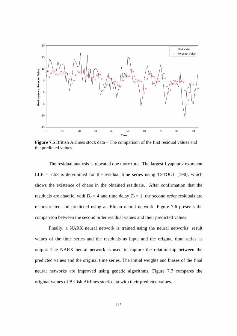
115

-15

-10

-5

0

5

10

15

20

0 10 20 30 40 50 60 70 80 90

Time

RealV

alu

evs.F

ore

cast

Valu

e

Real Value

Forecast Value

Figure 7.5 British Airlines stock data – The comparison of the first residual values andthe predicted values.

The residual analysis is repeated one more time. The largest Lyapunov exponent

LLE = 7.58 is determined for the residual time series using TSTOOL [190], which

shows the existence of chaos in the obtained residuals. After confirmation that the

residuals are chaotic, with D2 = 4 and time delay T2 = 1, the second order residuals are

reconstructed and predicted using an Elman neural network. Figure 7.6 presents the

comparison between the second order residual values and their predicted values.

Finally, a NARX neural network is trained using the neural networks’ result

values of the time series and the residuals as input and the original time series as

output. The NARX neural network is used to capture the relationship between the

predicted values and the original time series. The initial weights and biases of the final

neural networks are improved using genetic algorithms. Figure 7.7 compares the

original values of British Airlines stock data with their predicted values.

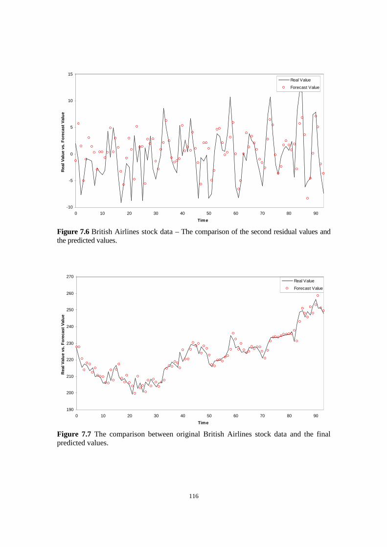
116

-10

-5

0

5

10

15

0 10 20 30 40 50 60 70 80 90

Time

RealV

alu

evs.F

ore

cast

Valu

e

Real Value

Forecast Value

Figure 7.6 British Airlines stock data – The comparison of the second residual values andthe predicted values.

190

200

210

220

230

240

250

260

270

0 10 20 30 40 50 60 70 80 90

Time

RealV

alu

evs.F

ore

cast

Valu

e

Real Value

Forecast Value

Figure 7.7 The comparison between original British Airlines stock data and the finalpredicted values.

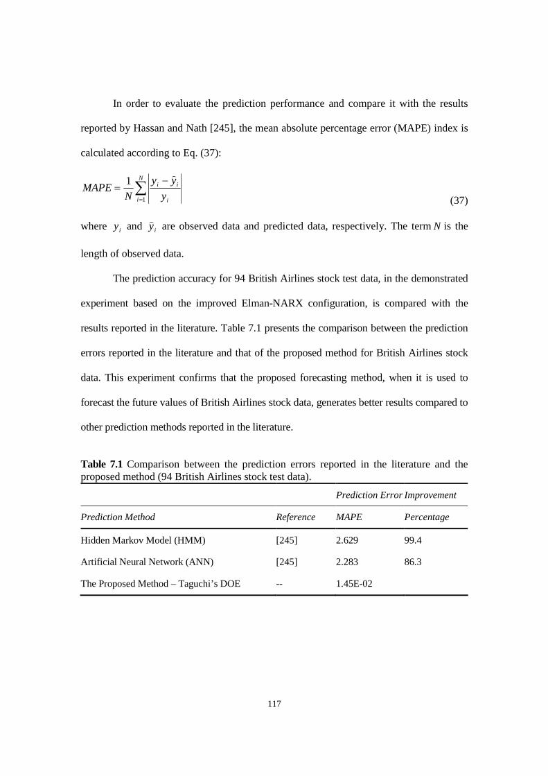
117


reported by Hassan and Nath [245], the mean absolute percentage error (MAPE) index is

calculated according to Eq. (37):

N

i i

ii

y

yy

NMAPE

1

1

(37)

where iy and iy

are observed data and predicted data, respectively. The term N is the

length of observed data.

The prediction accuracy for 94 British Airlines stock test data, in the demonstrated

experiment based on the improved Elman-NARX configuration, is compared with the

results reported in the literature. Table 7.1 presents the comparison between the prediction

errors reported in the literature and that of the proposed method for British Airlines stock

data. This experiment confirms that the proposed forecasting method, when it is used to

forecast the future values of British Airlines stock data, generates better results compared to

other prediction methods reported in the literature.

Table 7.1 Comparison between the prediction errors reported in the literature and theproposed method (94 British Airlines stock test data).


Prediction Method Reference MAPE Percentage

Hidden Markov Model (HMM) [245] 2.629 99.4

Artificial Neural Network (ANN) [245] 2.283 86.3

The Proposed Method – Taguchi’s DOE -- 1.45E-02

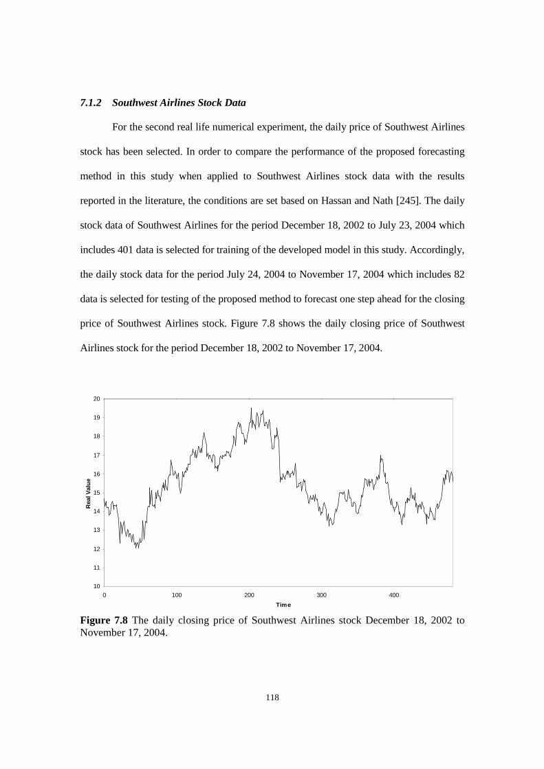
118

7.1.2 Southwest Airlines Stock Data

For the second real life numerical experiment, the daily price of Southwest Airlines

stock has been selected. In order to compare the performance of the proposed forecasting

method in this study when applied to Southwest Airlines stock data with the results

reported in the literature, the conditions are set based on Hassan and Nath [245]. The daily

stock data of Southwest Airlines for the period December 18, 2002 to July 23, 2004 which

includes 401 data is selected for training of the developed model in this study. Accordingly,

the daily stock data for the period July 24, 2004 to November 17, 2004 which includes 82

data is selected for testing of the proposed method to forecast one step ahead for the closing

price of Southwest Airlines stock. Figure 7.8 shows the daily closing price of Southwest

Airlines stock for the period December 18, 2002 to November 17, 2004.

10

11

12

13

14

15

16

17

18

19

20

0 100 200 300 400

Time

RealV

alu

e

Figure 7.8 The daily closing price of Southwest Airlines stock December 18, 2002 toNovember 17, 2004.

119

The first step in applying the proposed forecasting method to Southwest Airlines

stock data is to detect chaos in the time series. The largest Lyapunov exponent for

Southwest Airlines stock data is positive, LLE = 4.08, which indicates chaotic behaviour.

The original time series is reconstructed with embedding dimension D = 4 and

time delay T = 1. The embedded phase space points are fed into an Elman neural network

with 4 neurons in the input and output layers and 6 recurrent neurons and trained. The

weights and biases of the Elman neural network are kept to forecast the future values of

phase space points and consequently the original time series.


prediction. Based on a positive largest Lyapunov exponent, LLE = 7.26, it is concluded

that the first order residuals are chaotic. The first order residuals, are reconstructed with

embedding dimension D1 = 3 and time delay T1 = 1. The reconstructed phase space points

are fed into a new Elman neural network. The neural network is set up with 3 neurons in

the input and output layers and 6 neurons in the hidden layer. The residual analysis is

repeated one more time and it is concluded that the second order residuals show chaotic

behaviour, LLE = 7.67. With D2 = 3 and time delay T2 = 1, the future values of the second

order residuals are predicted based on the proposed prediction method. Finally, a NARX

network is trained using neural networks’ result values of the time series and the residuals

as input and the original time series as output. The last neural network is used to capture

the relationship between the neural networks’ result values and the original time series.

Figure 7.9 compares the original values of Southwest Airlines time series with their final

predicted values.

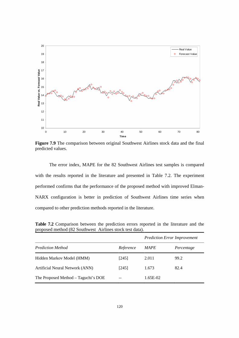
120

10

11

12

13

14

15

16

17

18

19

20

0 10 20 30 40 50 60 70 80

Time

RealV

alu

evs.F

ore

cast

Valu

e

Real Value

Forecast Value

Figure 7.9 The comparison between original Southwest Airlines stock data and the finalpredicted values.

The error index, MAPE for the 82 Southwest Airlines test samples is compared

with the results reported in the literature and presented in Table 7.2. The experiment

performed confirms that the performance of the proposed method with improved Elman-

NARX configuration is better in prediction of Southwest Airlines time series when

compared to other prediction methods reported in the literature.

Table 7.2 Comparison between the prediction errors reported in the literature and theproposed method (82 Southwest Airlines stock test data).






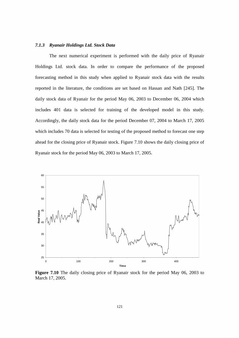
121

7.1.3 Ryanair Holdings Ltd. Stock Data

The next numerical experiment is performed with the daily price of Ryanair

Holdings Ltd. stock data. In order to compare the performance of the proposed

forecasting method in this study when applied to Ryanair stock data with the results

reported in the literature, the conditions are set based on Hassan and Nath [245]. The

daily stock data of Ryanair for the period May 06, 2003 to December 06, 2004 which

includes 401 data is selected for training of the developed model in this study.

Accordingly, the daily stock data for the period December 07, 2004 to March 17, 2005

which includes 70 data is selected for testing of the proposed method to forecast one step

ahead for the closing price of Ryanair stock. Figure 7.10 shows the daily closing price of

Ryanair stock for the period May 06, 2003 to March 17, 2005.

25

30

35

40

45

50

55

60

0 100 200 300 400

Time

RealV

alu

e

Figure 7.10 The daily closing price of Ryanair stock for the period May 06, 2003 toMarch 17, 2005.

122

The existence of chaos is investigated in Ryanair stock data. The value of the

largest Lyapunov exponent for Ryanair stock data is positive, LLE = 4.14, which is an

indication of chaotic behaviour in the data.

The embedding dimensions D = 3 and T = 1 are estimated as explained in Section

3.2.4 and 3.2.5 using TSTOOL [190]. Accordingly, phase space points are reconstructed.

An Elman neural network including 3 neurons in the input layer, 6 neurons in the hidden

layer, 6 recurrent neurons and 3 neurons in the output layer is trained. The weights and

biases of the network are kept for the purpose of prediction.

The prediction errors for the data selected for the training phase are calculated and

analyzed. The largest Lyapunov exponent, LLE = 7.04 is positive; therefore, it is concluded

that the residuals show chaotic behaviour. Based on this finding, the residuals are treated as

a new chaotic time series with embedding dimension D1 = 5 and time delay T1 = 1 and the

proposed method is applied to predict the future value of the residuals. The second level of

residual analysis is performed and the existence of chaos is detected in the residual time

series, LLE = 6.86. With the embedding dimension D2 = 3 and time delay T2 =1, the second

level residuals are predicted. Finally, a NARX network is trained using neural networks’

result values of the time series and the residuals as input and the original time series as

output to correlate the predicted values to the original time series. Figure 7.11 compares the

original values of Ryanair time series with their final predicted values.

The error index, MAPE, for the 70 Ryanair stock test samples are compared

with the results reported in the literature and presented in Table 7.3. The experiment

performed for Ryanair stock data confirms that the proposed method with the improved

123

Elman-NARX configuration performs better than other prediction methods reported in

the literature.

35

37

39

41

43

45

47

49

51

53

55

0 10 20 30 40 50 60

Time

RealV

alu

evs.F

ore

cast

Valu

e

Real Value

Forecast Value

Figure 7.11 The comparison between original Ryanair stock data and the final predictedvalues.

Table 7.3 Comparison between the prediction errors reported in the literature and theproposed method (70 Ryanair stock test data).






124

7.1.4 Lucent Incorporated Stock Data

The last numerical experiment performed on stock data in this study is the daily

stock price of Lucent incorporated. In order to compare the performance of the proposed

forecasting method in this study when applied to Lucent incorporated stock data with the

results reported in the literature, the conditions are set based on Afolabi and Olude [139].

The daily stock data of Lucent incorporated for the period November 28, 1998 to

November 28, 2003 which includes 1258 data is selected for training and testing of the

developed model in this study. Similar to Afolabi and Olude [139] the first 258 are

removed and the next 500 data are selected for training and the last 500 data are used to

test the performance of the proposed forecasting method. Figure 7.12 shows the scaled

daily closing price of Lucent stock for the period November 28, 1998 to November 28,

2003 scaled according to Afolabi and Olude [139].

-0.8

-0.6

-0.4

-0.2

0

0.2

0.4

0.6

0.8

0 100 200 300 400 500 600 700 800 900 1000 1100 1200

Time

RealV

alu

e

Figure 7.12 The scaled daily closing price of Lucent incorporated stock for the periodNovember 28, 1998 to November, 28 2003.

125

Lucent stock data are analyzed to detect chaos in the time series. The largest

Lyapunov exponent for Lucent stock data is positive, LLE = 4.29, which is an indication

of chaotic behaviour in the data. The original time series is reconstructed with the

embedding dimension D = 3 and time delay T = 8. The embedded phase space points are

fed into an Elman neural network with 3 neurons in the input and output layers and 6

recurrent neurons and trained. The weights and biases of the Elman neural network are kept

to forecast the future values of phase space points and consequently the original time series.


prediction. Based on a positive largest Lyapunov exponent, LLE = 6.56, it is concluded that

the first level residuals are chaotic. The first order residuals are reconstructed with the

embedding dimension D1 = 3 and time delay T1 = 1. The reconstructed phase space points

are fed into a new Elman neural network. The neural network is set up with 3 neurons in

the input and output layers and 6 neurons in the hidden layer. The residual analysis is

repeated one more time. The second level residuals are examined and with LLE = 6.56, the

existence of chaos is confirmed. With D2 = 3 and time delay T2 = 1, the future values of the

second order residuals are predicted based on the proposed prediction method. Finally, a

NARX network is trained using neural networks’ result values of the time series and the

residuals as input and the original time series as output. Figure 7.13 compares the scaled

values of Lucent time series with their final predicted values.

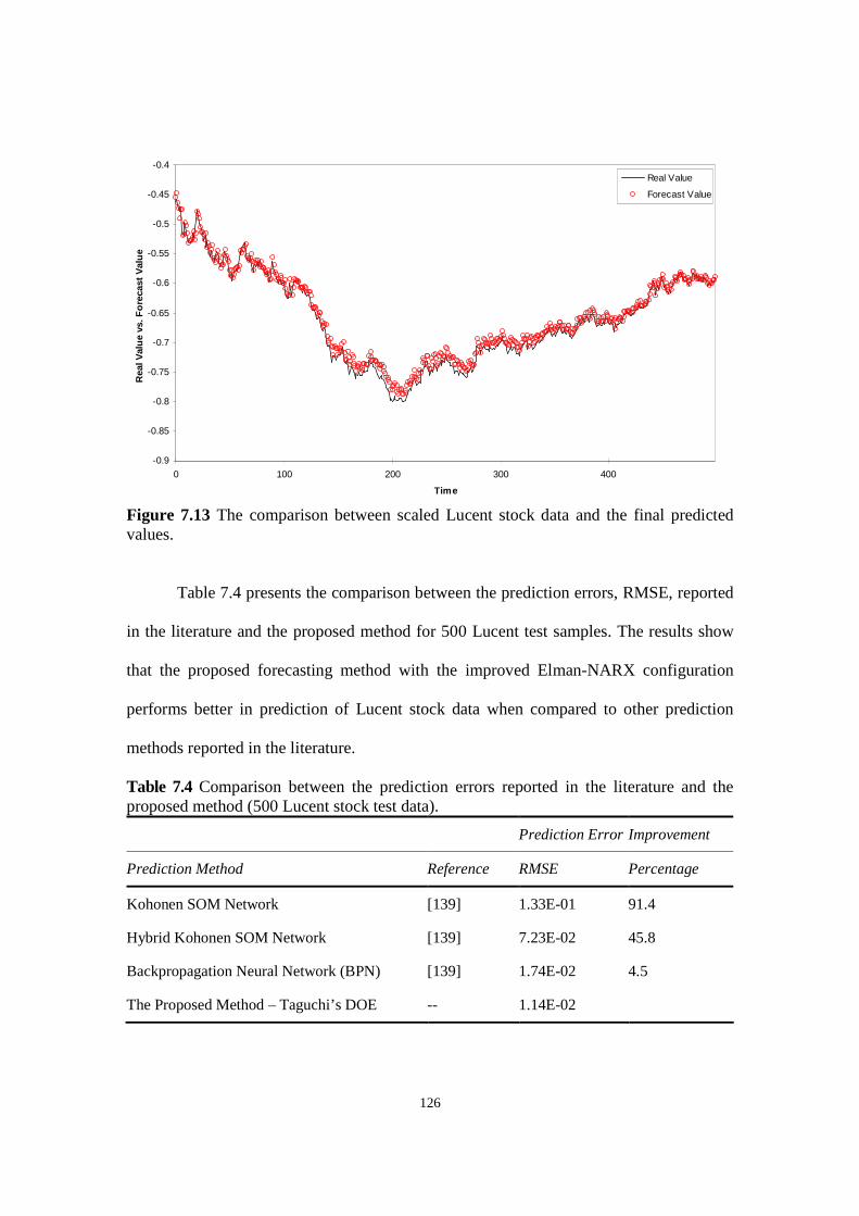
126

-0.9

-0.85

-0.8

-0.75

-0.7

-0.65

-0.6

-0.55

-0.5

-0.45

-0.4

0 100 200 300 400

Time

RealV

alu

evs.F

ore

cast

Valu

e

Real Value

Forecast Value

Figure 7.13 The comparison between scaled Lucent stock data and the final predictedvalues.

Table 7.4 presents the comparison between the prediction errors, RMSE, reported

in the literature and the proposed method for 500 Lucent test samples. The results show

that the proposed forecasting method with the improved Elman-NARX configuration

performs better in prediction of Lucent stock data when compared to other prediction

methods reported in the literature.

Table 7.4 Comparison between the prediction errors reported in the literature and theproposed method (500 Lucent stock test data).


Prediction Method Reference RMSE Percentage

Kohonen SOM Network [139] 1.33E-01 91.4

Hybrid Kohonen SOM Network [139] 7.23E-02 45.8

Backpropagation Neural Network (BPN) [139] 1.74E-02 4.5


127

7.2 Exchange Rates

Foreign exchange markets are one of the largest financial markets [255]. The

foreign exchange trades are happening 24 hours a day in financial markets [10]. Due to

the importance of foreign currencies, the exchange rates are important indicators in the

international financial markets [255]. A number of fundamental factors which change the

foreign exchange rates are the inflation in the concerned country, the supply of money,

the money market rate as a measurement for the short-term interest rate, the long-term

government bond yield and lending rate, which are the measurement for the long-term

interest rate, the rate of industrial production and the trade balance relative to the gross

domestic product (GDP) [10].

The exchange rate forecast models are generally categorized into two types:

fundamental and technical. The fundamental model is based on the feedback of the demand

and supply of domestic currency compared with a foreign currency. In the technical model,

the historical exchange rate data are required to determine the underlying structure of these

data and obtain the governing rules by which the time series data are produced [255,256].

The developed forecasting method in this study falls under technical models.

The evidence of complexity, nonlinearity and dynamical behaviour has been

observed in the exchange rate time series [257,258,259,260,261]. Cecen et al. [252] and

Bask [253,254] showed the existence of chaos in the exchange rate markets by obtaining

a positive Lyapunov exponent in the exchange rate time series. Richards [262] and

Schwartz and Yousefi [263] detected fractal properties in the exchange rate time series

and claimed chaotic behaviour in the exchange rate markets. Das and Das [10]

investigated nonlinearity and chaos in foreign exchange rates for twelve countries:

128

Australia, Canada, China, India, Japan, Malaysia, Singapore, Sri Lanka, Sweden,

Switzerland, Thailand and UK, over the span of nearly 36 years. Calculating the largest

Lyapunov exponent (LLE), Das and Das [10] found an indication of chaotic behaviour in

all the exchange rate time series.

A number of methods are introduced in the literature to forecast foreign exchange

rates. Tenti [102] proposed the application of recurrent neural networks to predict foreign

exchange rates. The method developed by Tenti was used to forecast the future of Deutsche

mark currency. Kim and Kim [154] used a genetic fuzzy predictor ensemble (GFPE)

method to forecast the exchange rates between the Swiss franc and the US dollar

(CHF/USD). Guegan and Mercier [264] developed two forecasting methods based on the

nearest neighbours and the radial basis function to forecast the daily exchange rates

between the Deutsche mark and the French franc (DEM/FRF). Liu [255] selected fuzzy

logic to study exchange rates between the US dollar and the Japanese yen (USD/JPY) and

developed a dynamic adaptive neuron-fuzzy logic forecasting model. Sheikhan and

Movaghar [73] proposed an evolutionary connectionist model in which GA is used to

improve the parameters and structure of the feedforward neural network. The proposed

method by Sheikhan and Movaghar [73] was applied to the daily exchange rates between

the Euro and the US dollar (EUR/USD) and the Euro and the Britain pound (EUR/GBP).

In this section, the proposed forecasting method using chaos theory, the embedding

theorem, residual analysis and improved ensemble neural networks with genetic algorithms

and Taguchi’s design of experiments is applied to daily exchange rates between the Euro

and the US dollar (EUR/USD) and the US dollar and the Japanese yen (USD/JPY).

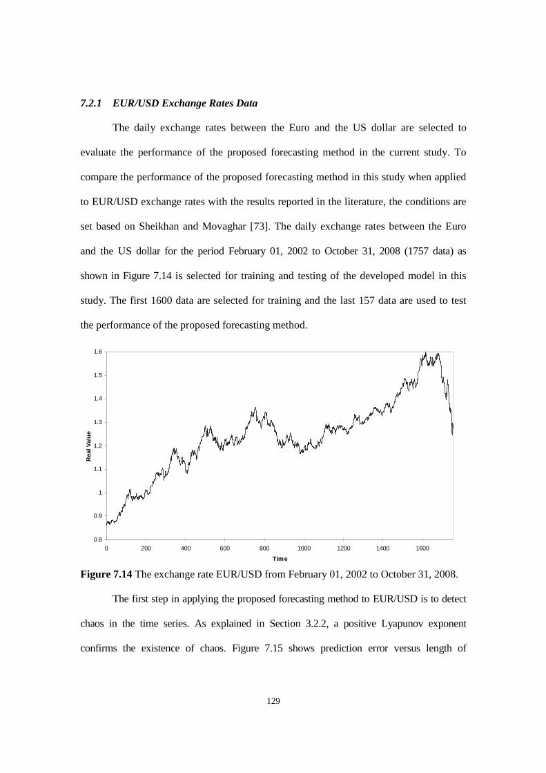
129

7.2.1 EUR/USD Exchange Rates Data

The daily exchange rates between the Euro and the US dollar are selected to

evaluate the performance of the proposed forecasting method in the current study. To

compare the performance of the proposed forecasting method in this study when applied

to EUR/USD exchange rates with the results reported in the literature, the conditions are

set based on Sheikhan and Movaghar [73]. The daily exchange rates between the Euro

and the US dollar for the period February 01, 2002 to October 31, 2008 (1757 data) as

shown in Figure 7.14 is selected for training and testing of the developed model in this

study. The first 1600 data are selected for training and the last 157 data are used to test

the performance of the proposed forecasting method.

0.8

0.9

1

1.1

1.2

1.3

1.4

1.5

1.6

0 200 400 600 800 1000 1200 1400 1600

Time

RealV

alu

e

Figure 7.14 The exchange rate EUR/USD from February 01, 2002 to October 31, 2008.

The first step in applying the proposed forecasting method to EUR/USD is to detect

chaos in the time series. As explained in Section 3.2.2, a positive Lyapunov exponent

confirms the existence of chaos. Figure 7.15 shows prediction error versus length of

130

prediction for EUR/USD data. The slope of the linear portion of the graph estimates the value

of the largest Lyapunov exponent (LLE). The largest Lyapunov exponent for EUR/USD data

is positive, LLE = 4.54, which is an indication of chaotic behaviour in the data.

Figure 7.15 Largest Lyapunov exponent graph for EUR/USD data.

The embedding dimension D and the time delay T are calculated using TSTOOL

[190]. EUR/USD data is reconstructed into phase space points with embedding dimension

D = 4 and time delay T = 1. The embedded phase space points are fed into an Elman neural

network with 4 neurons in the input and output layers and 6 hidden and recurrent neurons.

The weights and biases of the trained Elman neural network are kept to forecast the future

values of the phase space points and eventually the future values of EUR/USD data.

The prediction errors for the training data are calculated and analyzed. The largest

Lyapunov exponent, LLE = 8.86, is determined for the residual time series using TSTOOL

[190], which shows the existence of chaos in the obtained residuals. The residuals obtained

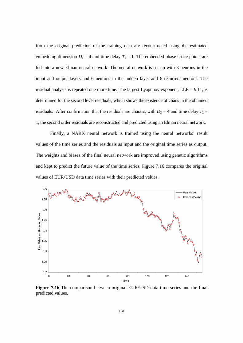
131

from the original prediction of the training data are reconstructed using the estimated

embedding dimension D1 = 4 and time delay T1 = 1. The embedded phase space points are

fed into a new Elman neural network. The neural network is set up with 3 neurons in the

input and output layers and 6 neurons in the hidden layer and 6 recurrent neurons. The

residual analysis is repeated one more time. The largest Lyapunov exponent, LLE = 9.11, is

determined for the second level residuals, which shows the existence of chaos in the obtained

residuals. After confirmation that the residuals are chaotic, with D2 = 4 and time delay T2 =

1, the second order residuals are reconstructed and predicted using an Elman neural network.

Finally, a NARX neural network is trained using the neural networks’ result

values of the time series and the residuals as input and the original time series as output.

The weights and biases of the final neural network are improved using genetic algorithms

and kept to predict the future value of the time series. Figure 7.16 compares the original

values of EUR/USD data time series with their predicted values.

1.2

1.25

1.3

1.35

1.4

1.45

1.5

1.55

1.6

0 20 40 60 80 100 120 140

Time

RealV

alu

evs.F

ore

cast

Valu

e

Real Value

Forecast Value

Figure 7.16 The comparison between original EUR/USD data time series and the finalpredicted values.

132

The error indices, MSE and NMSE for the 157 EUR/USD test samples are

compared with the results reported in the literature and presented in Table 7.5. The

experiment performed for the daily exchange rates between the Euro and the US dollar

confirms that the proposed method with improved Elman-NARX configuration has better

performance compared to other prediction methods reported in the literature.

Table 7.5 Comparison between the prediction errors reported in the literature and theproposed method (157 EUR/USD test data).

Prediction Error


Evolutionary Connectionist Model [73] 3.10E-03 5.00E-02

The Proposed Method – Taguchi’s DOE -- 1.43E-04 1.83E-02

7.2.2 USD/JPY Exchange Rates

The daily exchange rates between the US dollar and the Japanese yen are selected

for analysis and forecasting. In order to compare the performance of the proposed

forecasting method in this study when applied to USD/JPY data with the results reported

in the literature, the conditions are set based on Liu [255]. The daily exchange rates

between the US dollar and the Japanese yen for the period January 01, 2003 and

December 31, 2006 (1040 data) as shown in Figure 7.17 are selected for training and

testing of the developed model in this study. The first 540 data are selected for training

and the last 500 data are used to test the performance of the proposed forecasting method.

The largest Lyapunov exponent for USD/JPY data is positive, LLE = 5.22, which is

an indication of chaotic behaviour in the data. The embedding dimensions D = 3 and T = 5

are estimated as explained in Section 3.2.4 and 3.2.5 using TSTOOL [190]. Accordingly,

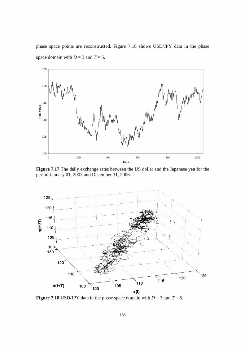
133

phase space points are reconstructed. Figure 7.18 shows USD/JPY data in the phase

space domain with D = 3 and T = 5.

100

105

110

115

120

125

0 200 400 600 800 1000

Time

RealV

alu

e

Figure 7.17 The daily exchange rates between the US dollar and the Japanese yen for theperiod January 01, 2003 and December 31, 2006.

Figure 7.18 USD/JPY data in the phase space domain with D = 3 and T = 5.

134

An Elman neural network is structured with 3 neurons in the input layer, 6

neurons in the hidden layer, 6 recurrent neurons and 3 neurons in the output layer and

then trained. The weights and biases of the network are kept for prediction purposes.

Figure 7.19 compares the real data with the predicated values for 94 data kept for testing.

The prediction errors for the data selected for the training are calculated and

analyzed. The largest Lyapunov exponent for the residual time series, LLE = 6.76, is

positive; therefore, it is concluded that the residuals exhibit chaotic behaviour. Based on

this finding, the residuals are treated as a new chaotic time series and the prediction

method proposed in Section 5.1 is applied to predict the future value of the residuals. The

first order residuals are reconstructed with embedding dimension D1 = 3 and time delay

T1 = 1. Figure 7.20 presents the residuals of the original prediction and the predicted

values for the test data.

100

105

110

115

120

125

0 100 200 300 400

Time

RealV

alu

evs.F

ore

cast

Valu

e

Real Value

Forecast Value

Figure 7.19 USD/JPY data – Comparing the original test data and the predicted values.

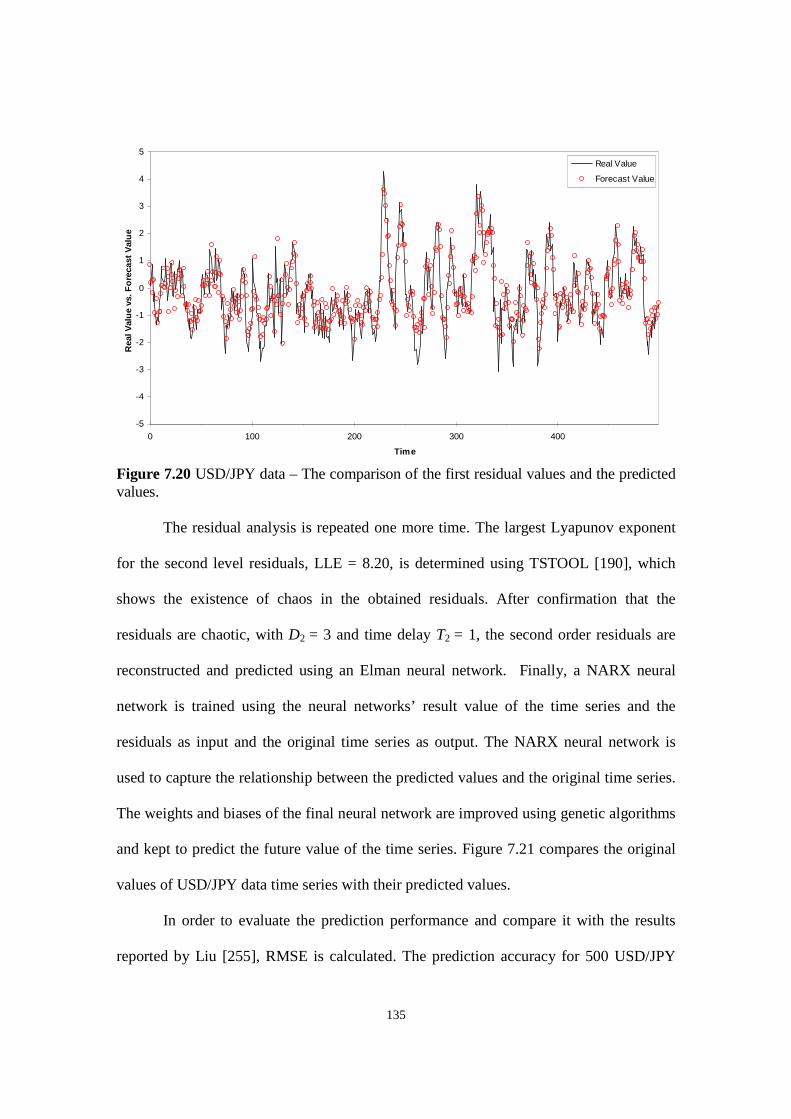
135

-5

-4

-3

-2

-1

0

1

2

3

4

5

0 100 200 300 400

Time

RealV

alu

evs.F

ore

cast

Valu

e

Real Value

Forecast Value

Figure 7.20 USD/JPY data – The comparison of the first residual values and the predictedvalues.

The residual analysis is repeated one more time. The largest Lyapunov exponent

for the second level residuals, LLE = 8.20, is determined using TSTOOL [190], which

shows the existence of chaos in the obtained residuals. After confirmation that the

residuals are chaotic, with D2 = 3 and time delay T2 = 1, the second order residuals are

reconstructed and predicted using an Elman neural network. Finally, a NARX neural

network is trained using the neural networks’ result value of the time series and the

residuals as input and the original time series as output. The NARX neural network is

used to capture the relationship between the predicted values and the original time series.

The weights and biases of the final neural network are improved using genetic algorithms

and kept to predict the future value of the time series. Figure 7.21 compares the original

values of USD/JPY data time series with their predicted values.


reported by Liu [255], RMSE is calculated. The prediction accuracy for 500 USD/JPY

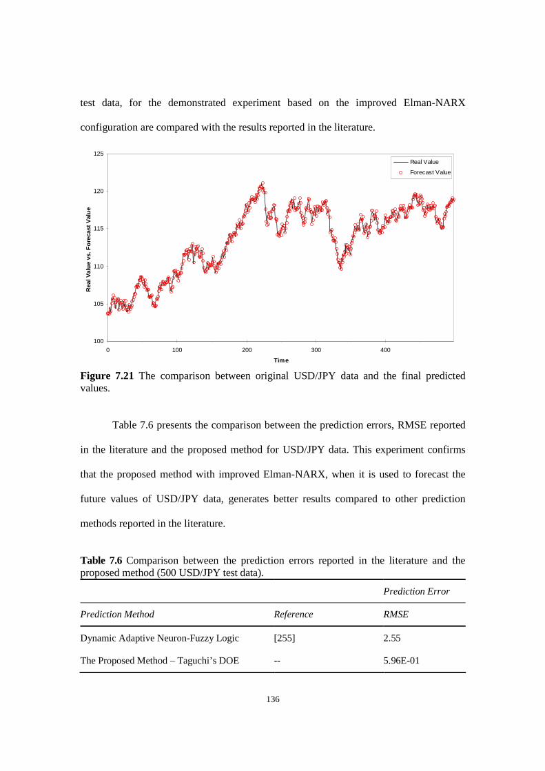
136

test data, for the demonstrated experiment based on the improved Elman-NARX

configuration are compared with the results reported in the literature.

100

105

110

115

120

125

0 100 200 300 400

Time

RealV

alu

evs.F

ore

cast

Valu

e

Real Value

Forecast Value

Figure 7.21 The comparison between original USD/JPY data and the final predictedvalues.

Table 7.6 presents the comparison between the prediction errors, RMSE reported

in the literature and the proposed method for USD/JPY data. This experiment confirms

that the proposed method with improved Elman-NARX, when it is used to forecast the

future values of USD/JPY data, generates better results compared to other prediction

methods reported in the literature.

Table 7.6 Comparison between the prediction errors reported in the literature and theproposed method (500 USD/JPY test data).

Prediction Error

Prediction Method Reference RMSE

Dynamic Adaptive Neuron-Fuzzy Logic [255] 2.55


137

7.3 Summary

The application of chaos theory is increasing in various disciplines. Chaos has

been observed in mixing processes, the control of robot servos, communications,

industry, economics, ecology, international relations, medicine, supply chain

management, inventory management, cardiovascular control system, hydrological field,

operations research and financial markets.

A robust technique to predict chaotic systems can increase the efficiency of the

system under study and decrease the risk. Chaotic system forecasting has been reported in

many areas such as financial markets, supply chain management, oil price and

consumption, power load, production systems and others. In financial markets, chaos

theory has been applied to commodity markets, stock markets and exchange rates among

others. The stock markets and foreign exchange markets are vital parts of the global

financial markets. The financial researchers closely studied the stock markets and foreign

exchange markets and observed the evidence of complexity, nonlinearity and dynamical

behaviour in both markets.

In this chapter, the forecasting method developed with the residual analysis

method using ensemble neural networks and improved by genetic algorithms and

Taguchi’s design of experiments was applied to financial markets, namely, stock markets

and exchange rate trading. The daily price of four stocks, namely, British Airlines,

Southwest Airlines, Ryanair Holdings and Lucent Incorporated and two exchange rates,

namely, EUR/USD and USD/JPY were analyzed and their future values were predicted.

In all the numerical experiments, the proposed forecasting method shows better

performance compared to the results reported in the literature.

138

CHAPTER 8

CONCLUSION AND FUTURE WORK

8.1 Conclusion

Chaos theory has been used to study and analyze chaotic systems. Chaotic systems

generate random-look data; however, in the embedding phase space, they present

deterministic behaviour. Forecasting chaotic time series has increasingly become a

popular and challenging subject. Many of the forecasting methods proposed in the

literature are either inefficient when applied to chaotic time series, or difficult to

implement. The motivation to conduct the current study was to develop a more effective,

easy-to-use and practical method to forecast chaotic time series.

In this study, an original technique was developed to forecast one step ahead of a

given chaotic time series. The key difference between this technique and the techniques

proposed in the literature was the utilization of the precise definition of chaos theory and

the embedding theorem. Chaos theory states that, for a chaotic system, there exists an

unknown mathematical equation which can describe the system. Also, the embedding

theorem claims that in phase space mode, a chaotic system reflects most of the

characteristics of the original system. Therefore, the unknown state of the given chaotic

system can be replaced by the generated phase space points. Also, the unknown function

which governs the original system can be estimated with a neural network. In the current

technique, an artificial neural network was trained using a single phase space point

139

(current state) as input and a single phase space point (next state) as output. This

complies precisely with the definition of chaos theory and the embedding theorem.

The first step to proceed with the proposed forecasting method was to determine

the existence of chaos in a given time series. When the presence of chaos was detected in

the observed time series, then the phase space parameters were calculated and the phase

space points were generated. An artificial neural network with a single phase space point,

D input units, and a single phase space point, D output units, was trained. After training

the artificial neural network, the weights and biases of the network were kept to forecast

the unknown phase space points and obtain the future values of chaotic time series.

In order to evaluate the performance of the proposed method, the developed

technique was applied to three chaotic time series: Mackey-Glass, Logistic and Henon. The

feedforward neural network and the Elman recurrent neural network were used to estimate

the unknown chaotic function. In most training algorithms, the initial weights and biases of

the neural network are selected randomly. This can cause variation in the output of the

neural network. To reduce the variation of the neural network output and select proper

initial weights and biases for the neural network, genetic algorithms were adopted. The

GA’s objective function was to minimize the mean square error (MSE) of the predicted

values based on the proposed technique and the original time series. The decision variables

were weights and biases of the neural network. When the GA was applied, the best weights

and biases which improved the performance of the neural network were selected. The

combination of the proposed forecasting method along with genetic algorithms presented

an outstanding result. The comparison between the result of the proposed technique and the

results reported in the literature substantiates the effectiveness of the proposed method.

140

Through an extensive analysis, it was observed that, in some cases, heuristic models

could not completely capture the characteristics of the original time series and, therefore,

the residuals became highly correlated. The residuals resulting from the developed neural

network prediction method were further analyzed, and it was observed that, in some cases,

they demonstrate chaotic behaviour.

To investigate the contribution of the residual analysis in improving the performance

of the proposed forecasting method, the obtained residuals were considered as a new chaotic

time series and analyzed separately. When the presence of chaos was confirmed in the

residual time series, the embedding dimension and the time delay were determined and the

phase space points were generated. A new artificial neural network, with D1 input units and

D1 output units, was trained and the future values of the residuals were obtained.

To correlate the neural networks’ result values of the time series and the residuals to

the original time series, a new neural network was trained. The neural network with two

input units and one output unit was trained. The neural networks’ result values of the time

series and the residuals were used as input and the original time series as output. To

increase the accuracy of the prediction, the residual analysis could be repeated several

times. To correlate the neural networks’ result values of the time series and the residuals in

various levels to the original time series, a neural network with M+1 input units, where M

is the level of residual analysis, and one output unit, could be trained. As before, the

proposed method was merged with genetic algorithms to improve the forecasting results.

To examine the performance of the proposed method, a feedforward-feedforward

configuration was applied to two simulated chaotic systems: Mackey-Glass and Lorenz

equations. Also, an Elman-NARX configuration was applied to the Mackey-Glass and

141

Lorenz equations and to one real life time series, sunspot time series. Despite its simplicity

in implementation, the proposed model exhibited a superior performance in prediction of

chaotic time series when compared with the results reported in the literature.

Taguchi’s design of experiments as an efficient approach to identify appropriate

factor-level combinations was utilized to improve the result of the proposed forecasting

method. A systematic approach was introduced using Taguchi’s design of experiments to

improve the combination selection of ensemble artificial neural networks and their

parameters. The method was applied to two benchmarking time series, the Mackey-Glass

and Lorenz, and two real life chaotic time series, namely, sunspot and far-infrared NH3

laser time series. The conclusion of Taguchi’s DOE for all four time series revealed that

among eight selected factors, Tier Neural Network Architecture, Final Neural Network

Architecture, Tier Network Training Method and Final Network Training Method

showed importance and their selected levels were Elman, NARX, traingdx and trainlm.

The experimental results confirmed that the selected levels identified by Taguchi’s DOE

improved the performance of the proposed forecasting method when compared with the

same method using arbitrary selection of artificial neural network architectures and


The proposed forecasting method was applied to financial markets, namely, stock

markets and exchange rate. The daily price of British Airlines, Southwest Airlines, Ryanair

Holdings and Lucent Inc. and two exchange rates, namely, EUR/USD and USD/JPY were

analyzed and predicted. In all the numerical experiments, the proposed forecasting method

based on improved Elman-NARX configuration using Taguchi’s DOE and GA showed

better performance compared to the results reported in the literature.

142

8.2 Contributions

The main objective of this research work was to develop an easy-to-use, effective

and practical method to forecast chaotic time series. This goal was achieved by proposing

an easy-to-use forecasting method which exhibits superior performance when compared

with other forecasting methods in the literature.

The following represents the contribution of this research work:

After extensive review of the literature, it was noted that none of the existing

approaches makes full use of the precise definition of chaos theory, which

requires a single phase space point as input and a single phase space point as

output. Therefore, the precise definition of chaos theory and the embedding

theorem was adopted to develop an effective forecasting method. This version of

the proposed forecasting method showed better performance when compared with

similar methods in the literature.

A thorough analysis of residuals was conducted to investigate the characteristics

of the residuals. The investigation demonstrated that chaos was present in some of

the test problems. Therefore, the method was further enhanced by incorporating

the residual analysis into the proposed forecasting method.

Several neural network architectures were utilized in this study, and the impact of

the various architectures on the efficiency and effectiveness of the proposed

forecasting method was examined. The main application of artificial neural

networks is to estimate the unknown underlying function governing the system

under study and capture the relationships among the given data. Feedforward

neural networks from a static category and Elman and NARX neural networks

143

from a dynamic category were selected for the analysis. It was concluded that the

dynamic architectures in the proposed configuration perform better compared to

the static neural networks.

In this study, genetic algorithms have been adopted to select the initial weights

and biases of artificial neural networks to improve the performance of the

networks. The numerical examples substantiated that genetic algorithms can

enhance the effectiveness of the proposed forecasting method by selecting proper

initial weights and biases for the selected artificial neural networks.

Several configurations and parameters are involved in the structure of the

proposed forecasting method. Design of experiments (DOE) is a well-known

method to select a proper combination of the parameters to optimize the result.

Taguchi’s DOE, as an efficient method in selecting appropriate factor-level

combination was adopted to improve the performance of the proposed method.

A systematic approach based on Taguchi’s DOE was introduced to facilitate the

combination selection of the ensemble artificial neural networks and their

parameters. The numerical examples demonstrated that the improved forecasting

method using Taguchi’s DOE performs better when compared with the same

method using an arbitrary selection of artificial neural network architectures and


Several benchmarking and a couple of real life chaotic time series are selected for

numerical experiments. An extensive literature review was performed to compare

the performance of the proposed forecasting method with the various forecasting

models in the literature. The comparison between the results obtained in this study

144

and the results reported in the literature established the superiority and

effectiveness of the proposed forecasting method.

Stock markets and exchange rate markets are the essential and important parts of

the global economics. The existence of chaos has been observed in both markets.

Forecasting the future of these markets can facilitate planning and decision

making in these areas and reduce the associated risks. The forecasting method

proposed in this research was applied to both stock markets and foreign exchange

rates. The obtained results confirmed that the proposed forecasting method is an

easy-to-use, effective and practical method to forecast the future of stock markets

and the exchange rate markets.

8.3 Future work

This dissertation presented an original method to forecast chaotic time series more

effectively and accurately. The results of the numerical experiments confirmed that the

proposed method performed better than other forecasting models in the literature in the

investigated areas. However, to further improve the quality of the current study, the

followings can be investigated as an extension to this research work.

In this study, only two levels of residual analysis were examined. In all examined

numerical experiments, two levels of residual analysis delivered better

performance when compared with the results presented in the literature. In future

work, this can be extended to more levels of residual analysis to increase the

accuracy of forecasting.

145

Application of chaos theory has been observed in many fields such as

communications, ecology, international relations, medicine, hydrological field,

supply chain management and financial markets. In this study, the proposed

forecasting method was applied to some benchmarking and real life chaotic time

series. Also, in financial section, the developed forecasting method was applied to

stock markets and foreign exchange rates. This can be extended in future work to

other fields such as supply chain management, product design, inventory

management and demand forecasting.

There are several factors and parameters involved in the design of the proposed

forecasting method. These factors consist of the neural network architecture,

neural network parameters, embedding parameters and genetic algorithm

parameters. In the current study, Taguchi’s design of experiments was employed

to improve the performance of the proposed forecasting method by selecting the

appropriate level of the involved factors. Among all the involved factors and

parameters, only the impact of the neural network architecture, transfer function,

and training method in two levels were studied in this research. The impact of

other factors can be investigated and more levels can be selected for the factors.

The forecasting method developed in this study has been applied to stock market

and exchange rate data. In future work, the proposed forecasting method can be

utilized in loss and profit analysis and portfolio management.

In the current study, the number of training and test data are selected according to

the literature to be able to compare the performance of the proposed method with

the results reported in the literature. In future work, the optimum proportion of

146

training and test data can be determined. Also, in the proposed method, the trained

neural network is used to forecast all the test data. An investigation can be

conducted to determine when the forecasting performance drops and the neural

networks require re-training.

The validity of the proposed can be tested on other types of time series such as

deterministic, stationary, non-stationary, seasonal, stochastic and other.

In the current study, only univariate chaotic time series are analyzed. The

application of the proposed forecasting method can be extended to multivariate

chaotic time series.

The current research work is applied to forecast one step ahead of chaotic time

series. The performance of the proposed forecasting method for long term

prediction of chaotic time series can be investigated.

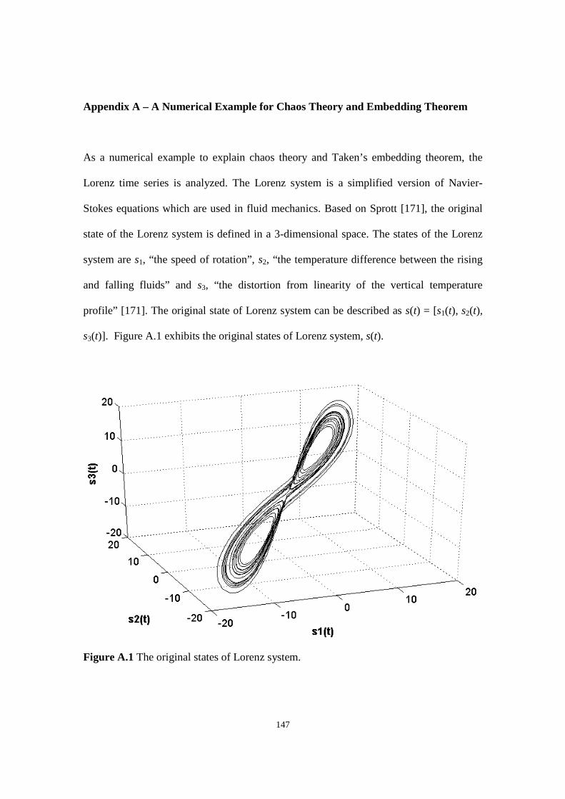
147

Appendix A – A Numerical Example for Chaos Theory and Embedding Theorem

As a numerical example to explain chaos theory and Taken’s embedding theorem, the

Lorenz time series is analyzed. The Lorenz system is a simplified version of Navier-

Stokes equations which are used in fluid mechanics. Based on Sprott [171], the original

state of the Lorenz system is defined in a 3-dimensional space. The states of the Lorenz

system are s1, “the speed of rotation”, s2, “the temperature difference between the rising

and falling fluids” and s3, “the distortion from linearity of the vertical temperature

profile” [171]. The original state of Lorenz system can be described as s(t) = [s1(t), s2(t),

s3(t)]. Figure A.1 exhibits the original states of Lorenz system, s(t).

Figure A.1 The original states of Lorenz system.

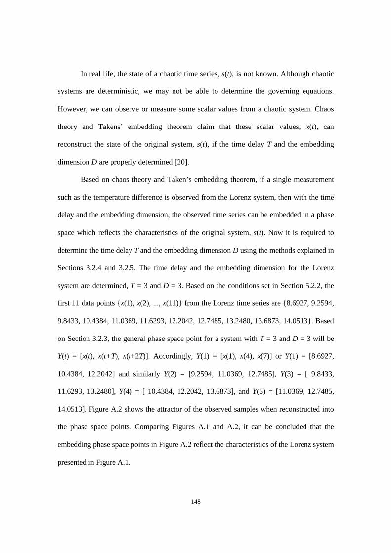
148

In real life, the state of a chaotic time series, s(t), is not known. Although chaotic

systems are deterministic, we may not be able to determine the governing equations.

However, we can observe or measure some scalar values from a chaotic system. Chaos

theory and Takens’ embedding theorem claim that these scalar values, x(t), can

reconstruct the state of the original system, s(t), if the time delay T and the embedding

dimension D are properly determined [20].

Based on chaos theory and Taken’s embedding theorem, if a single measurement

such as the temperature difference is observed from the Lorenz system, then with the time

delay and the embedding dimension, the observed time series can be embedded in a phase

space which reflects the characteristics of the original system, s(t). Now it is required to

determine the time delay T and the embedding dimension D using the methods explained in

Sections 3.2.4 and 3.2.5. The time delay and the embedding dimension for the Lorenz

system are determined, T = 3 and D = 3. Based on the conditions set in Section 5.2.2, the

first 11 data points {x(1), x(2), ..., x(11)} from the Lorenz time series are {8.6927, 9.2594,

9.8433, 10.4384, 11.0369, 11.6293, 12.2042, 12.7485, 13.2480, 13.6873, 14.0513}. Based

on Section 3.2.3, the general phase space point for a system with T = 3 and D = 3 will be

Y(t) = [x(t), x(t+T), x(t+2T)]. Accordingly, Y(1) = [x(1), x(4), x(7)] or Y(1) = [8.6927,

10.4384, 12.2042] and similarly Y(2) = [9.2594, 11.0369, 12.7485], Y(3) = [ 9.8433,

11.6293, 13.2480], Y(4) = [ 10.4384, 12.2042, 13.6873], and Y(5) = [11.0369, 12.7485,

14.0513]. Figure A.2 shows the attractor of the observed samples when reconstructed into

the phase space points. Comparing Figures A.1 and A.2, it can be concluded that the

embedding phase space points in Figure A.2 reflect the characteristics of the Lorenz system

presented in Figure A.1.

149

Figure A.2 Lorenz time series reconstructed into the phase space points with T = 3 andD = 3.

150

Appendix B – A Numerical Example to Detect the Existence of Chaos

Four methods are introduced in Section 3.2.2 to determine the presence of chaos in a given

time series. In this section, the Henon time series which has been used in the literature as a

benchmark time series is selected to demonstrate how the existence of chaos can be

detected in a given time series. The details of the Henon time series are given in Section

4.2.3. The Henon time series with 1000 data points is shown in Figure B.1.

Figure B.1 Henon chaotic time series with 1000 data points.

The first method which is utilized to investigate the existence of chaos is Fourier

transform or a power spectrum plot. As highlighted in Section 3.2.2, the spectrum for

chaotic time series will be broadband with a broad peak. Figure B.2 is a power spectrum

plot for the Henon time series. Figure B.2 confirms the presence of chaos in the Henon

time series as the power spectrum is broadband with a broad peak.

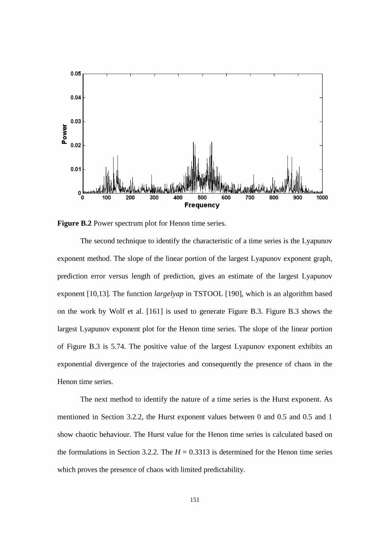
151

Figure B.2 Power spectrum plot for Henon time series.

The second technique to identify the characteristic of a time series is the Lyapunov

exponent method. The slope of the linear portion of the largest Lyapunov exponent graph,

prediction error versus length of prediction, gives an estimate of the largest Lyapunov

exponent [10,13]. The function largelyap in TSTOOL [190], which is an algorithm based

on the work by Wolf et al. [161] is used to generate Figure B.3. Figure B.3 shows the

largest Lyapunov exponent plot for the Henon time series. The slope of the linear portion

of Figure B.3 is 5.74. The positive value of the largest Lyapunov exponent exhibits an

exponential divergence of the trajectories and consequently the presence of chaos in the

Henon time series.

The next method to identify the nature of a time series is the Hurst exponent. As

mentioned in Section 3.2.2, the Hurst exponent values between 0 and 0.5 and 0.5 and 1

show chaotic behaviour. The Hurst value for the Henon time series is calculated based on

the formulations in Section 3.2.2. The H = 0.3313 is determined for the Henon time series

which proves the presence of chaos with limited predictability.

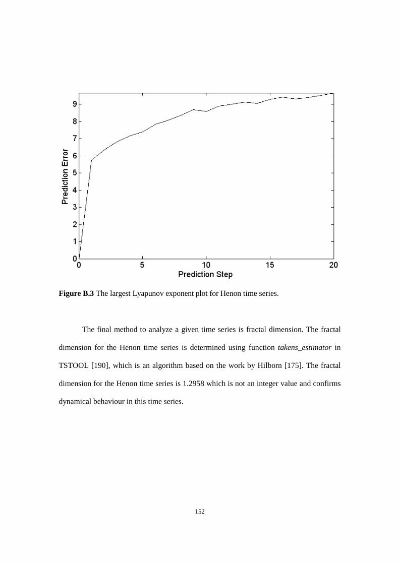
152

Figure B.3 The largest Lyapunov exponent plot for Henon time series.

The final method to analyze a given time series is fractal dimension. The fractal

dimension for the Henon time series is determined using function takens_estimator in

TSTOOL [190], which is an algorithm based on the work by Hilborn [175]. The fractal

dimension for the Henon time series is 1.2958 which is not an integer value and confirms

dynamical behaviour in this time series.

153

Appendix C – A Numerical Example to Determine Embedding Parameters

To use Taken’s [20] embedding theorem, it is essential to calculate embedding

parameters, namely, time delay and embedding dimension. The formulations presented in

Section 3.2.4 and 3.2.5 and TSTOOL [190], an add-on toolbox for MATLAB [191] are

utilized to determine T and D.

As mentioned in Section 3.2.4, average mutual information is a suitable method to

identify the time delay for a given chaotic time series. The function amutual in TSTOOL

[190], which is an algorithm based on the work by Abarbanel [62] is used to generate

Figure C.1. Time delay for the Henon time series based on the average mutual

information graph in Figure C.1 is T = 1.

Figure C.1 Average mutual information graph for Henon time series.

154

The next step after selecting the time delay is to determine the embedding

dimension. The embedding dimension for the Henon time series is determined using

function cao in TSTOOL [190], which is an algorithm based on Cao’s method [176].

Based on the graph generated using Cao’s method shown in Figure C.2, there is a kink at

2. Therefore, for the Henon time series the embedding dimension is D = 2.

Figure C.2 Cao’s graph to identify embedding dimension for Henon time series.

When the presence of chaos is identified in a time series and embedding

parameters are determined, the time series is reconstructed into the phase space points.

Using time delay T = 1 and embedding dimension D = 2, the Henon time series is

reconstructed into the phase space points. Figure C.3 shows the Henon time series in the

phase space domain.

155

Figure C.3 Henon time series in phase space domain.

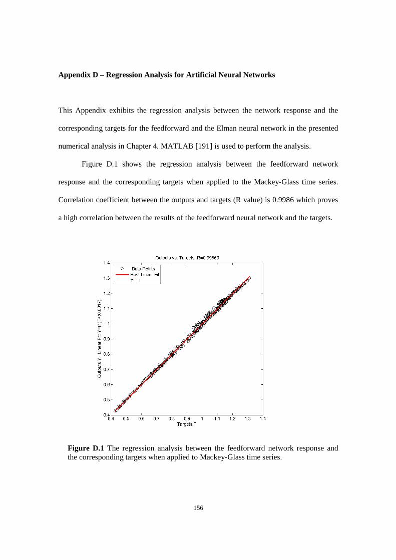
156

Appendix D – Regression Analysis for Artificial Neural Networks

This Appendix exhibits the regression analysis between the network response and the

corresponding targets for the feedforward and the Elman neural network in the presented

numerical analysis in Chapter 4. MATLAB [191] is used to perform the analysis.

Figure D.1 shows the regression analysis between the feedforward network

response and the corresponding targets when applied to the Mackey-Glass time series.

Correlation coefficient between the outputs and targets (R value) is 0.9986 which proves

a high correlation between the results of the feedforward neural network and the targets.

Figure D.1 The regression analysis between the feedforward network response andthe corresponding targets when applied to Mackey-Glass time series.

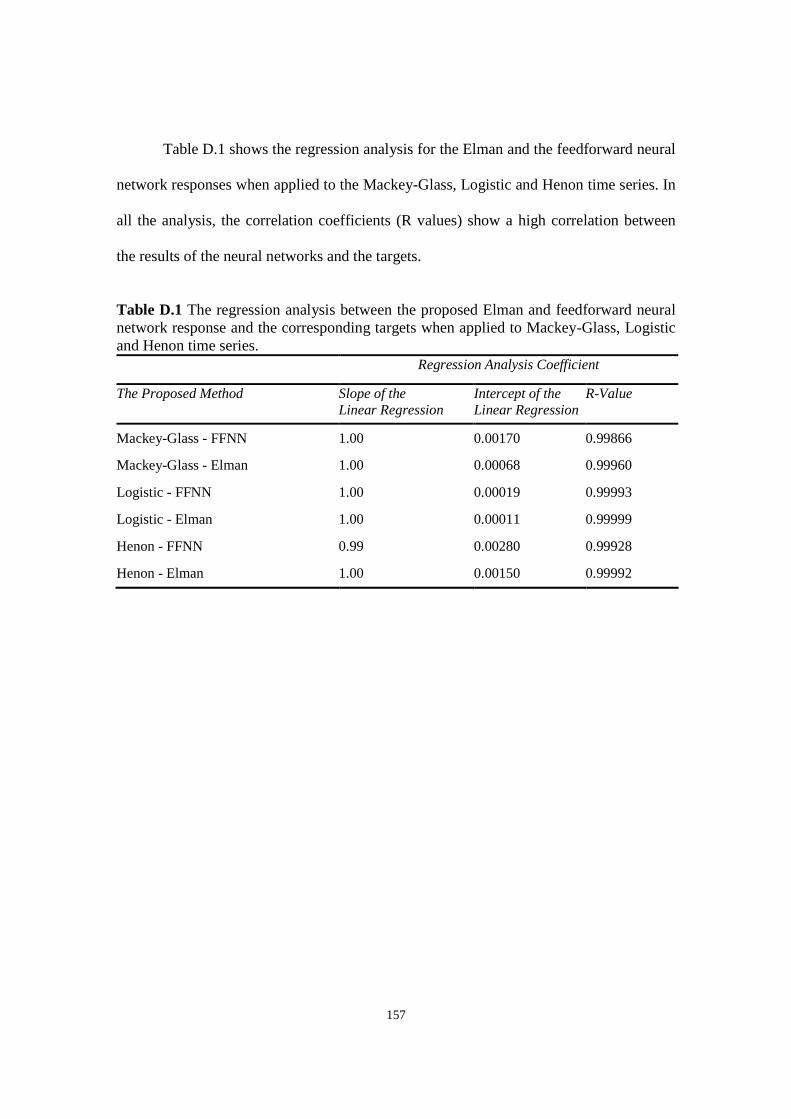
157

Table D.1 shows the regression analysis for the Elman and the feedforward neural

network responses when applied to the Mackey-Glass, Logistic and Henon time series. In

all the analysis, the correlation coefficients (R values) show a high correlation between

the results of the neural networks and the targets.

Table D.1 The regression analysis between the proposed Elman and feedforward neuralnetwork response and the corresponding targets when applied to Mackey-Glass, Logisticand Henon time series.

Regression Analysis Coefficient

The Proposed Method Slope of theLinear Regression

Intercept of theLinear Regression

R-Value

Mackey-Glass - FFNN 1.00 0.00170 0.99866

Mackey-Glass - Elman 1.00 0.00068 0.99960

Logistic - FFNN 1.00 0.00019 0.99993

Logistic - Elman 1.00 0.00011 0.99999

Henon - FFNN 0.99 0.00280 0.99928

Henon - Elman 1.00 0.00150 0.99992

158

REFERENCES

[1] Zhang, J., Man, K.F. (1998) Time series prediction using recurrent neural network in

multi-dimension embedding phase space. IEEE International Conference on Systems,

Man, and Cybernetics. Vol. 2, pp. 11–14.

[2] Aref, H. (1984) Stirring by chaotic advection. Journal of Fluid Mechanics. Vol. 143,

pp.1–21.

[3] Aubry, N., Holmes, P.J., Lumley, J.L., Stone, E. (1988) The dynamics of coherent

structures in the wall region of a turbulent boundary layer. Journal of Fluid

Mechanics. Vol. 192, pp.115–173.

[4] MacKay, R.S. (1993) Some thoughts on chaos in engineering. 7th Toyota Conference:

Toward the Harnessing of Chaos. Shizuoka, Japan.

[5] Erramilli, A., Forys, L.J. (1991) Oscillations and chaos in a flow model of a switching

system. IEEE Journal of information systems: Logistics Information Management.

Vol. 6 (4), pp.15–25.

[6] Uzunoglu, V., White, M.H. (1985) The synchronous oscillator: a synchronization and

tracking network. IEEE Journal of Solid State Circuits. Vol. 20(6), pp. 1214–1225.

[7] Scott, S. (1991) Chemical Chaos. Oxford University Press.

[8] Weiss, G. (1992) Chaos hits Wall Street – the theory that is. Business Week.

November 2, pp. 138–140.

[9] Qian, B., Rasheed, K. (2007) Stock market prediction with multiple classifiers.

Applied Intelligence. Vol. 26, pp. 25–33.

[10] Das, A., Das, P. (2007) Chaotic analysis of the foreign exchange rates. Applied

Mathematics and Computation. Vol. 185, pp. 388–396.

[11] Kennel, M.B. (1992) Method to distinguish possible chaos from colored noise and to

determine embedding parameters. Physical Review A. Vol. 46, pp. 3111–3118.

[12] Wilding, R. (1998) Chaos, complexity and supply-chains. Logistics Focus. Vol. 6, pp. 8–10.

[13] Nair, A.S., Liu, J.C., Rilett, L., Gupta, S. (2001) Non-linear analysis of traffic flow.

In Proceedings of IEEE Intelligent Transportation Systems Conference. pp. 25–29.

[14] Kawauchi, S., Sugihara, H., Sasaki, H. (2004) Development of very-short-term load

forecasting based on chaos theory. Electrical Engineering in Japan. Vol. 148(2),

pp. 55–63.

159

[15] Lorenz, E.N. (1993) The Essence of Chaos. Seattle, University of Washington Press.

[16] Park, Y.R., Murray, T.J., Chen, C. (1996) Predicting sun spots using a layered

perceptron neural network. IEEE Transactions on Neural Networks. Vol. 1(2), pp.

501–505.

[17] González, J.J., Pereda, E. (2004) Applications of fractal and non-linear time series

analysis to the study of short-term cardiovascular control. Current Vascular

Pharmacology., Vol. 2, pp. 149–162.

[18] Casdagli, M. (1991) Chaos and deterministic versus stochastic non-linear modelling.

in: Journal Royal Statistics Society: Series B, Vol. 54(2), pp.303–328.

[19] Wilding, R. (1998) Chaos theory: implications for supply chain management.

International Journal of Logistics Management. Vol. (9), pp. 43–56.

[20] Takens, F. (1981) Detecting strange attractors in turbulence. in Dynamic Systems

and Turbulence, Lecture Notes in Mathematics. Vol. (898), pp.366–381.

[21] Frazier, C., Kockelman, K. M. (2004) Chaos theory & transportation systems: an

instructive example. Transportation Research Record. Vol. (1897), pp. 9–17.

[22] Martinez-Rego, D., Fontenla-Romero, O., Alonso-Betanzos, A. (2008) A method for

time series prediction using a combination of linear models. In Proceedings of

European Symposium on Artificial Neural Network – Advances in Computational

Intelligence and Learning, Bruges, Belgium.

[23] Casdagli M. (1989) Nonlinear prediction of chaotic time series. Physica D. Vol. 35,

pp. 335–356.

[24] Farmer, J.D., Sidorowic, J.J. (1987) Predicting chaotic time series. Physical Review

Letters. Vol. 8(59), pp. 845–848.

[25] McNames, J., (1998) A nearest trajectory strategy for time series prediction. In

Proceedings of International Workshop on Advanced Black-Box Techniques for

Nonlinear Modelling. Katholieke Universiteit Leuven, Belgium, pp. 112–128.

[26] Liu, F., Quek, C., Ng, G.S. (2005) Neural network model for time series prediction

by reinforcement learning. In Proceedings of International Joint Conference on

Neural Networks. Vol. 2, pp. 809–814.

160

[27] Ma, Q., Zheng, Q., Peng, H., Zhong, T., Xu, L. (2007) Chaotic time series prediction

based on evolving recurrent neural networks. In Proceedings of Sixth International

Conference on Machine Learning and Cybernetics. Hong Kong.

[28] Menezes, J.M., and Barreto, G.A. (2008) Long-term time series prediction with the

NARX network: an empirical evaluation. Neurocomputing. Vol. 71, pp. 3335–3343.

[29] Diaconescu, E., (2008) The use of NARX neural networks to predict chaotic time

series. WSEAS Transactions on Computer Research. Vol. 3 (3), pp. 182–191.

[30] Tao, D., Xiao, H. (2007) Chaotic time series prediction based on radial basis

function network. In Proceedings of 8th ACIS International Conference on

Software Engineering, Artificial Intelligence, Networking, and Parallel/Distributed

Computing. Vol. 1, pp. 595–599.

[31] Rojas, I., Valenzuelab, O., Rojasa, F., Guillena, A., Herreraa, L.J., Pomaresa, H.,

Marquezb, L., Pasadasb, M. (2008) Soft-computing techniques and ARMA model

for time series prediction. Neurocomputing. Vol. 71, pp. 519–537.

[32] Koskela, T., Varsta, M. Heikkonen, J. Kaski, S. (1998) Time series prediction using

recurrent SOM with local linear models. International Journal of Knowledge-based

Intelligent Engineering Systems. Vol. 2(1), pp. 60–68.

[33] Barreto, G.A. (2006) Time series prediction with the self-organizing map: A review.

Perspectives on Neural-Symbolic Integration. Vol. 77, pp. 135–158.

[34] Sapankevych, N., Sankar, R. (2009) Time series prediction using support vector

machines: A survey. IEEE Computational Intelligence Magazine. Vol. 4 (2), pp. 24–38.

[35] Wang, X., Zhang, H., Zhang, C., Cai, X., Wang, J. (2005) Prediction of chaotic time

series using LS-SVM with automatic parameter selection. In Proceedings of Sixth

International Conference on Parallel and Distributed Computing – Applications

and Technologies. pp. 962–965.

[36] Szpiro, G. (1997) Forecasting chaotic time series with genetic algorithms. Physical

Review E. Vol. 55(3), pp. 2557–2568.

[37] Meyer, T., Packard, N.H. (1992) in Nonlinear Modeling and Forecasting, edited by

M. Casdagli and S. Eubanks, SFI Studies in the Sciences of Complexity , Addison–

Wesley, New York , pp. 249–264.

161

[38] Kodogiannis, V., Lolis, A. (2002) Forecasting financial time series using neural

network and fuzzy system-based techniques. Neural Computing and Applications.

Vo.11, pp. 90–102.

[39] Zhang, J., Chung, H. S., Lo, W. (2008) Chaotic time series prediction using a neuro-

fuzzy system with time-delay coordinates. IEEE Transactions on Knowledge and

Data Engineering. Vol. 20(7), pp. 956–964.

[40] Garcia-Trevino, E.S., Alarcon-Aquino, V. (2006) Single-step prediction of chaotic

time series using wavelet-networks. In Proceedings of Electronics, Robotics and

Automotive Mechanics Conference. Vol. 1, pp. 243–248.

[41] Wang, Y., Jiang, W., Yuan, S., Wang, J. (2008) Forecasting chaotic time series

based on improved genetic Wnn. In Proceedings of Fourth International

Conference on Natural Computation. Jinan, China.

[42] Wichard, J.D., Ogorzalek M. (2004) Time series prediction with ensemble models.

In Proceedings of the IJCNN. Vol. 2, pp.1625–1629.

[43] Kim, Y.S., Yum, B.J. (2004) Robust design of multilayer feedforward neural

networks: an experimental approach. Engineering Applications of Artificial

Intelligence. Vol. 17(3), pp. 249–263.

[44] Khaw, J.F.C., Lim, B.S., Lim, L.E.N. (1995) Optimal design of neural networks

using Taguchi method. Neurocomputing. Vol. 7(3), pp. 225–245.

[45] Lin, T.Y., Tseng, C.H. (2000) Optimum design for artificial neural networks: an

example in a bicycle derailleur system. Engineering Applications of Artificial

Intelligence. Vol. 13(1), pp. 3–14.

[46] Ortiz-Rodríguez, J.M., Martínez-Blanco, M.R., Vega-Carrillo, H.R. (2006) Robust

design of artificial neural networks applying the Taguchi methodology and DOE.

Proceedings of Electronics, Robotics and Automotive Mechanics Conference. Vol. 3,

pp. 131–136.

[47] Packianather, M.S., Drake, P.R. (2004) Modelling neural network performance

through response surface methodology for classifying wood veneer defects.

Proceedings of the Institution of Mechanical Engineers, Part B: Journal of

Engineering Manufacture. Vol. 218(4), pp. 459–466.

162

[48] Wang, Q., Stockton, D.J., Baguley, P. (2000) Process cost modeling using neural

networks. International Journal of Production Research. Vol. 38(16), pp. 3811–3821.

[49] Yang, S.M., Lee, G.S. (1999) Neural network design by using Taguchi method.

Journal of Dynamic Systems, Measurement, and Control. Vol. 121, pp. 560–563.

[50] Peterson, G.E., St. Clair, D.C., Aylward, S., Bond, W. (1995) Using Taguchi´s

method of experimental design to control errors in layered perceptrons. IEEE

Transactions on Neural Networks. Vol. 6(4), pp. 949–961.

[51] Mouli, K.C., Srinivas, J., Subbaiah, K.V. (2006) Optimisation and output forecasting

using Taguchi-neural network approach. J. of the Institution of Engineers. pp. 54–57.

[52] Newton, I. (1729) The Mathematical Principles of Natural Philosophy. trans. A.

Motte. Benjamin Motte, London.

[53] Wilding, R.D. (1997) An Investigation into Sources of uncertainty within Industrial

Supply Chains; Amplification, Deterministic Chaos & Parallel Interactions. PhD

Dissertation, University of Warwich.

[54] Stewart, I. (1989) Does God Play Dice? Penguin, London.

[55] Crutchfield, J.P., Farmer, J.D., Packard, N.H. and Shaw, R.S. (1986) Chaos.

Scientific America. Vol. 254 (12), pp. 46–57.

[56] Campbell, L., Garnett, W. (1882) The Life of James Clerk Maxwell. MacMillan and

Co., London.

[57] Cartwright, M.L. (1965) Jacques Hadamard, 1865-1963. The Royal Society.

[58] Peitgen, H.O., Jurgens, H., Saupe, D. (1992) Chaos and Fractals: New Frontiers of

Science, Springer-Velag, New York.

[59] Li, T.Y., Yorke J.A. (1975) Period three implies chaos. American Mathematical

Monthly. Vol. 82(10), pp. 985–992

[60] Stacey, R.D. (1993) Strategic Management and Organizational Dynamics. Pitman

Publishing, London.

[61] Kaplan, D., Glass, L. (1995) Understanding Nonlinear Dynamics, Springer-Verlag, NY.

[62] Abarbanel, H. (1996) Analysis of Observed Chaotic Data. Spinger-Verlag, New York.

[63] Box, G.E.P., Jenkins, G.M. (1976) Time Series Analysis, Forecasting and Control.

Holden-Day, Oakland, CA, Revised version.

163

[64] Pollok, D.S.G. (1999) A Handbook of Time Series, Signal Processing and

Dynamics. Academic Press, London.

[65] Regonda, S.K., Rajagopalan, B., Lall, U., Clark, M., Moon, Y.I. (2005) Local

polynomial method for ensemble forecast of time series. Nonlinear Processes in

Geophysics. Vol. 12, pp. 397–406.

[66] Lau, K.W., Wu, Q.H. (2008) Local prediction of non-linear time series using support

vector regression. Pattern Recognition. Vol. 41, pp. 1556–1564.

[67] Khashei, M., Bijari, M., Raissi Ardali, G.A. (2009) Improvement of auto-Regressive

integrated moving average models using fuzzy logic and artificial neural networks

(ANNs). Neurocomputing. Vol. 72, pp. 956–967.

[68] Thissen, U., Brakel, R., Weijer, A.P., Melssen, W.J., Buydens, L.M.C. (2003) Using

support vector machines for time series prediction. Chemometrics and Intelligent

Laboratory Systems. Vol. 69, pp. 35– 49.

[69] Zhang, W., Wu, Z., Yang, G. (2004) Genetic programming-based chaotic time series

modeling. Journal of Zhejiang University Science. Vol. 5(11), pp. 1432–1439.

[70] Edmonds, A.N. (1996) Time series prediction using supervised learning and tools

from chaos theory. PhD Dissertation, University of Luton.

[71] Jayawardena, A.W., Lai, F. (1993) Chaos in hydrological time series. Proceedings of

the Yokohama Symposium – Extreme Hydrological Events: Precipitation, Floods

and Droughts. pp.59–66.

[72] Sannasiraj, S.A., Zhang, H., Babovic, V. Chan, E.S. (2004) Enhancing tidal

prediction accuracy in a deterministic model using chaos theory. Advances in Water

Resources. Vol. 27, pp. 761–772.

[73] Sheikhan, M., Movaghar B. (2009) Exchange rate prediction using an evolutionary

connectionist model. World Applied Sciences Journal. Vol. 7, pp. 8–16.

[74] Gleick, J. (1987) Chaos - Making a new science. Viking, New York.

[75] Boné, R., Crucianu, M. (2002) Multi-step-ahead prediction with neural networks: a

review. In 9emes rencontres internationales: Approches Connexionnistes en

Sciences. Boulogne, France. pp. 97–106.

164

[76] Bontempi, G, Birattari, M., Bersini, H. (1999) Local learning for iterated time-series

prediction. Proceedings of the Sixteenth International Conference on Machine

Learning. San Francisco, USA, pp. 32–38.

[77] Lorenz, E.N. (1969) Atmospheric predictability as revealed by naturally occurring

analogues. Journal of the Atmospheric Sciences. Vol. 26, pp. 636-646.

[78] Jacobs, R.A., Jordan, M.I., Nowlan, S.J., Hinton, G.E. (1991) Adaptative mixtures of

local experts. Neural Computation. Vol. 3, pp. 79–87.

[79] Zhang, J., Man K. F., Ke J.Y. (1998) Time series prediction using Lyapunov

exponents in embedding phase space. Proceedings Fourth International

Conference on Signal Processing. Vol. 1, pp. 221–224.

[80] Chudy, L., Farkas, I. (1998) Prediction of chaotic time-series using dynamic cell

structures and local linear models. Neural Network World. Vol. 8(5), pp. 481–489.

[81] Kugiumtzis, D., Lingjaerde, O.C., Christophersen, N. (1998) Regularized local

linear prediction of chaotic time series. Physica D. Vol. 112, pp. 344–360.

[82] Sello, S. (2001) Solar cycle forecasting: a nonlinear dynamics approach. Astronomy

& Astrophysics. Vol. 377, pp. 312–320.

[83] Fontenla-Romero, O., Alonso-Betanzos, A., Castillo, E., Principe, J.C., Guijarro-

Berdinas, B. (2002) Local modeling using self-organizing maps and single layer

neural networks. In Lecture Notes in Computer Science. Vol. 2415, pp. 945–950.

[84] Gholipour, A., Araabi, B.N., Lucas, C. (2006) Predicting chaotic time series using

neural and neurofuzzy models: a comparative study. Neural Processing Letters,

Vol. 24, pp. 217–239.

[85] Granger, C.W.J., Anderson A.P (1978) An Introduction to Bilinear Time Series

Models, Vandenhoeck and Ruprecht, Gottingen.

[86] Subba-Rao, T., Gabr M.M. (1984) An introduction to bispectral analysis and bilinear

time series models. Lecture Notes in Statistics. Vol. 24, pp. 270–275.

[87] Ozaki, T., Oda, H. (1978) Nonlinear time series model identification by Akaike’s

information criterion. Information and Systems. pp. 83–91.

[88] Haggan, V. and T. Ozaki (1981) Modeling nonlinear random vibrations using an amplitude-

dependent autoregressive time series model, Biometrika. Vol. 68, pp. 189–196.

165

[89] Priestley, M.B. (1980) State dependent models: a general approach to nonlinear time

series analysis. Journal of Time Series Analysis. Vol. 1, pp. 57–71.

[90] Priestley, M.B. (1988) Non-linear and Non-stationary Time Series Analysis.

Academic Press, London.

[91] Tong, H., Lin, K.S. (1980) Threshold auto-regression, limit cycles and cyclical data.

Journal of the Royal Statistical Society. Vol. 42(3), pp. 245–292.

[92] Tong, H. (1983) Threshold Models in Nonlinear time Series Analysis. Springer

Verlag, New York.

[93] Martinez, T.M., Berkovich, S.G., Schulten, K.J. (1993) Neural-gas network for

vector quantization and its application to time-series prediction. IEEE Transactions

on Neural Networks. Vol. 4, pp. 558–569.

[94] Bersini, H., Birattari, M., Bontempi, G. (1998) Adaptive memory-based regression

methods. In Proceedings of the IEEE International Joint Conference on Neural

Networks. pp. 2102–2106.

[95] Girard, A., Rasmussen, C.E., Qui, J. (2003) Gaussian process priors with uncertain

inputs–Application to multiple-step ahead time series forecasting. In Advances in

Neural Information Processing Systems. Vol. 15, pp. 529–536.

[96] Jaeger, H., Haas, H. (2004) Harnessing nonlinearity: Predicting chaotic systems and

saving energy in wireless communication. Science. Vol. 304 (5667), pp. 78–80.

[97] Chen, Y., Yang, B., Dong, J., Abraham, A. (2005), Time-series forecasting using

flexible neural tree model. Information Sciences. Vol. 174, pp. 219–235.

[98] Chen, Y.M, Lin, C. (2007) Dynamic parameter optimization of evolutionary

computation for on-line prediction of time series with changing dynamics. Applied

Soft Computing. Vol. 7, pp. 1170–1176.

[99] Elsner, J.B., (1992) Predicting time series using a neural network as a method of

distinguishing chaos from noise, Journal of Physics A: Mathematical and General.

25 (4), pp. 843–850.

[100] Veelen, M., Nijhuis, J., Spaanenburg, B. (2000) Neural network approaches to

capture temporal information. In Computing Anticipatory Systems – Third

International Conference. Vol. 517, pp. 361–371.

166

[101] Moller, M. (1993) A scaled conjugate gradient algorithm for fast supervised

learning. Neural Networks. Vol. 6, pp. 525–533.

[102] Tenti, P. (1996) Forecasting foreign exchange rates using recurrent neural

networks. Applied Artificial Intelligence. Vol. 10, pp. 567–581.

[103] Connor, J., Atlas, L. (1991) Recurrent neural networks and time series prediction.

IEEE International Joint conference on Neural Networks. pp. 301–306.

[104] Connor, J.T., Martin D. (1994) Recurrent neural networks and robust time series

prediction. IEEE Transactions on Neural Networks. Vol. 5(2), pp. 240 – 254.

[105] Bone, R., Crucianu, M., Verley, G., Asselin de Beauville, J.P. (2000) A bounded

exploration approach to constructive algorithms for recurrent neural networks. In

Proceedings of IJCNN. Como, Italy, Vol. 3, pp. 27–30.

[106] Han, M., Xi, J., Xu, S., Yin, F. (2004) Prediction of chaotic time series based on

the recurrent predictor neural network. IEEE Transactions on Signal Processing.

Vol. 52(12), pp. 3409–3416.

[107] Assaad, M., Boné, R., Cardot, H. (2006) Predicting chaotic time series by boosted

recurrent neural networks. In Proceedings of International Conference on Neural

Information Processing. Vol. 4233, pp. 831–840.

[108] Guan, X., Mural, R.J., Uberbacher, E.C. (1994) Protein structure prediction using

hybrid AI methods. In Proceedings of the Tenth Conference on Artificial

Intelligence for Applications. pp. 471–473.

[109] Lin, J., Bartal, Y., Uhrig, R. (1995) Using similarity based formulas and genetic

algorithms to predict the severity of nuclear power plant transients. 9th Power Plant

Dynamics, Control & Testing Symposium. Knoxville, TN, pp. 53.01–53.09.

[110] Leung, H. (2001) Prediction of noisy chaotic time series using an optimal radial

basis function neural network. IEEE Transactions on Neural Networks. Vol. 12(5),

pp. 1163–1172.

[111] Haykin S., Principe, J. (1998) Making sense of a complex world. IEEE Signal

Processing Magazine. Vol. 15(3), pp. 66–68.

167

[112] Cowper, M.R., Mulgrew, B., Unsworth, C.P. (2002) Nonlinear prediction of

chaotic signals using a normalized radial basis function network. Signal

Processing. Vol. 82(5), pp. 775–789.

[113] Poggio, T., Girosi, F. (1989) A theory of networks for approximation and learning.

Massachusetts Institute of Technology, Cambridge, MA.

[114] Girosi, F., Jones, M., Poggio, T. (1995) Regularization theory and neural network

architectures. Neural Computation. Vol. 7(2), pp. 219–269.

[115] Cho, K.B., Wang, H.B. (1996) Radial basis function based adaptive fuzzy systems

and their applications to system identification and prediction. Fuzzy Sets and

Systems. Vol. 83(3), pp. 325–339.

[116] Rojas, I., Pomares, H., Bernier, J.L., Ortega, J., Pino, B., Pelayo, F.J., Prieto, A.

(2002) Time series analysis using normalized PG-RBF network with regression

weights, Neurocomputing. Vol. 42, pp. 267–285.

[117] Vesin, J.M. (1993) An amplitude-dependent autoregressive signal model based on a

radial basis function expansion. IEEE International Conference on Acoustics,

Speech, and Signal Processing. Vo. 3, pp. 129–132.

[118] Shi, Z., Y. Tamura, and T. Ozaki (1999) Nonlinear time series modelling with the

radial basis function-based state-dependent autoregressive model. International

Journal of Systems Science. Vol. 30(7), pp. 717–727.

[119] Peng, H., Ozaki, T., Toyoda, Y., Oda, K. (2001) Nonlinear system identification

using radial basis function-based signal-dependent ARX models. Proceedings of 5th

IFAC Symposium on Nonlinear Control Systems. Saint-Petersburg, Russia, pp. 703–708.

[120] Peng, H., Ozaki, T., Haggan-Ozaki, V. and Toyoda, Y. (2003) A parameter

optimization method for radial basis function type models. IEEE Transactions on

Neural Networks. Vol. 14, pp. 432–438.

[121] Haggan-Ozaki, V., Ozaki, T. Toyoda, Y. (2006) RBF-ARX modeling for prediction

and control. 14th IFAC Symposium on System Identification. Newcastle, Australia,

pp. 1210–1215.

168

[122] Teo, K., Wang, L., Lin, Z. (2001) Wavelet packet multi-layer perceptron for

chaotic time series prediction: effects of weight initialization. Computational

Science. Vol. 2074, pp. 310–317.

[123]Cao, L., Hong, Y., Fang, H. and He G. (1995) Predicting chaotic time series with

wavelet networks. Physica D: Nonlinear Phenomena. Vol. 85 (1-2), pp. 225–238.

[124] Gao, X., Xiao, F., Zhang, J., Cao, C. (2004) Short-term prediction of chaotic time

series by wavelet networks. Proceedings of the 5th World Congress on Intelligent

Control and Automation. Hangzhou, China, Vol. 3, pp. 1931–1935.

[125] Gao,X., Xiao, F. (2004) Multiwavelet networks for prediction of chaotic time series. IEEE

International Conference on Systems, Man and Cybernetics. Vol. 4, pp. 3328–3332.

[126] Wan, E.A. (1994) Time series prediction by using a connectionist network with

internal time delays. in Time Series Prediction: Forecasting the Future and

Understanding the Past. Addison-Wesley, pp. 195–217.

[127] Koskela, T., Lehtokangas, M. Saarinen, J., Kaski, K. (1996) Time series prediction

with multilayer perceptron, FIR and Elman neural networks. In Proceedings of

World Congress on Neural Networks. pp. 491–496.

[128] Day, S.P., Davenport, M.R. (1993) Continuous-time temporal backprogagation with

adaptive time delays. IEEE Transactions on Neural Networks. Vol. 4, pp. 348–354.

[129] Yao, X., Liu, Y. (1997) A new evolutionary system for evolving artificial neural

networks. IEEE Transactions on Neural Networks. Vol. 8(3), pp. 694–713.

[130] Hecht-Nielsen, R. (1988) Applications of countepropagation networks. Neural

Networks. Vol. 1, pp. 131–139.

[131] Fierascu, C. (2005) Counterpropagation with Delays with applications in time

series prediction. Artificial Neural Networks: Formal Models and Their

Applications. Vol. 3697, pp. 533–539.

[132] Gomez-Ramırez , E., Najim, K., Ikonen, E. (2007), Forecasting time series with a

new architecture for polynomial artificial neural network. Applied Soft Computing.

Vol. 7, pp. 1209–1216.

[133] Smola, A.J., Scholkopf, B. (1998) A tutorial on support vector regression.

Technical report. Statistics and Computing. Vol. 14 (3), pp. 199 – 222.

169

[134] Muller, K.R., Smola, A.J., Ratsch, G., Scholkopf, B., Kohlmorgen, J., Vapnik, V.

N. (1997) Predicting time series with support vector machines. In Proceedings of

7th International Conference of Artificial Neural Networks. Lausanne,

Switzerland, Vol. 1327, pp. 999–1004.

[135] Mukherjee, S., Osuna, E. and Girosi, F. (1997) Nonlinear prediction of chaotic time

series using support vector machines. In Proceedings of 7th IEEE Workshop

Neural Networks Signal Processing. Amelia Island, FL, pp. 511–520.

[136] Cao, L.J., Tay, F.E.H. (2003) Support vector machine with adaptive parameters in

financial time series forecasting. IEEE Transactions on Neural Networks. Vol.

14(6), pp. 1506–1518.

[137] Zheng, D., Wang, J., Zhao, Y. (2006) Time series predictions using multi-scale

Support Vector Regressions. Theory and Applications of Models of Computation.

Vol. 3959, pp. 474–481.

[138] Simon, G., Lendasse, A., Cottrell, M., Fort, J.C., Verleysen, M. (2005) Time series

forecasting: obtaining long term trends with self-organizing maps. Pattern

Recognition Letters. Vol. 26(12), pp. 1795–1808.

[139] Afolabi, M.O., Olude, O. (2007) Predicting stock prices using a hybrid Kohonen

self organizing map (SOM). Proceedings of the 40th Hawaii International

Conference on System Sciences. pp. 48.

[140] Zorin, A. (2003) Stock price prediction: Kohonen versus backpropagation. In

Proceedings of the International Conference on Modeling and Simulation of

Business Systems. Vilnius, Lithuania, pp. 115–119.

[141] Vesanto, J. (1997) Using the SOM and local models in time-series prediction. In

Proceedings of Workshop on Self-Organizing Maps. Espoo, Finland, pp. 209–214.

[142] Lee, K.L. and Billings, S.A. (2002) Time series prediction using support vector

machines, the orthogonal and the regularized orthogonal least-squares algorithms.

International Journal of Systems Science. Vol. 33(10), pp. 811–821.

[143] Shi, Z. and Han, M. (2007) Support vector echo-state machine for chaotic, time

series prediction. IEEE Transactions on Neural Networks. Vol. 18(2), pp. 359–372.

170

[144] Palit, A.K., Popovic, D. (1999) Forecasting chaotic time series using neuro-fuzzy

approach. International Joint Conference on Neural Networks. Washington D.C.,

USA, Vol.3, pp. 1538–1543.

[145] Jang, J.S.R., Sun, C.T. and Mizutani, E. (1997) Neuro-Fuzzy and Soft Computing.

Englewood cliffs, New Jersey, Prentice-Hall.

[146] Falco, I., Iazzetta, A., Natale, P., Tarantino, E. (1998) Evolutionary neural

networks for nonlinear dynamics modelling. In Parallel Problem Solving from

Nature. pp. 593–602.

[147] Yoshihara, I., Ohta, K., Yamamori, K. (2003) Construction of GMDH-based

prediction model using GA. Mem Fac Eng Miyazaki Univ. Vol. 32, pp.315–320.

[148] Luo, X. Heywood, M. and Zincir-Heywood, A.N. (2006) Benchmarking a recurrent

linear GP model on prediction and control problems, intelligent control and

automation. International Conference on Intelligent Computing. Kunming, China,

Vol. 344, pp. 845–850.

[149] Day, P., Nandi, A.K. (2008) Sunspot prediction using genetic programming augmented

by binary string fitness characterisation and comparative partner selection. IEEE

Workshop on Machine Learning for Signal Processing. pp. 175–180.

[150] Jia-shu, Z., Xian-Ci, X. (2000) Predicting low-dimensional chaotic time series

using volterra adaptive filer. Acta Physica Sinica. Vol. 49(3), pp. 403–408.

[151] Jia-shu, Z., Xian-Ci, (2000) Prediction of chaotic time series by using adaptive

higher-order nonlinear Fourier infrared filter. Acta Physica Sinica. Vol. 49(7), pp.

1221–1227.

[152] Jia-shu, Z., Xian-Ci, (2000) Nonlinear adaptive prediction of chaotic time series

with a reduced parameter nonlinear adaptive filter. Acta Physica Sinica. Vol.

49(12), pp. 2333–2339.

[153] Li, C., Yu, J. (2008) Volterra-TLS method for chaotic time series prediction.

International Conference on Communications, Circuits and Systems. pp. 48–51.

[154] Kim, D. and Kim, C. (1997) Forecasting time series with genetic-fuzzy predictor

ensemble. IEEE Transactions on Fuzzy Systems. Vol. 5(4), pp. 523–535.

171

[155] Bakker, R., Schouten, J.C., Giles, C.L., Takens, F., Bleek, C.M. (2000) Learning chaotic

attractors by neural networks. Neural Computation. Vol. 12(10), pp. 2355–2383.

[156] Fanzi, Z. Zhengding, Q. (2003) Predicting chaotic time series by ensemble self

generating neural networks merged with genetic algorithm. Proceedings of the

2003 International Conference on Neural Networks and Signal Processing.

Nanjing, China, Vol. 1, pp. 776–778.

[157] Bouchachia, A., Bouchachia, S. (2008) Ensemble learning for time series

prediction. The First International Workshop on Nonlinear Dynamic Systems and

Synchronization. pp. 1–8.

[158] Forrester, J.W. (1961) Industrial Dynamics, Systems Dynamics Series. Productivity

Press (MIT Press), Portland, Oregon.

[159] Thompson, J.M.T., Stewart, H.B. (1986) Nonlinear Dynamics and Chaos. John

Wiley & Sons, UK.

[160] Gordon, T., Greenspan, D. (1994) The Management of chaotic systems.

Technological Forecasting and Social Change. Vol. 47, pp. 49–62.

[161] Wolf, A., Swift, J.B., Swinney, H.L., Vastano, J.A. (1985) Determining Lyapunov

exponents from a time series. Physica D. Vol. 16(3), pp. 285–317.

[162] Banerjee, S. (1993) Choas. Students Journal of the Institute of Electronics and

Telecommunications Engineers. Vol. 34, pp. 39–50.

[163] Parker, D., Stacey, R. (1994) Chaos management and economics – the Implications

of Non-linear Thinking. Hobart Paper 125, Institute of Economic Affairs, London.

[164] Goldratt, E.M., Cox, J. (1984) The Goal. 2nd Ed., Gower Publishing, London.

[165] Vliet, A. (1994) Order from chaos. Management Today. November, pp. 62–67.

[166] Norgaard, M., Ravn, O., Poulsen, N.K., Hansen, L.K. (2000) Neural Networks for

Modelling and Control of Dynamic Systems. Springer, Berlin.

[167] Kantz, H., Scheiber, T. (1997) Nonlinear Time Series Analysis. Cambridge

University Press, Cambridge.

[168] Camilleri, M. (2004) Forecasting using non-linear techniques in time series

analysis: an overview of techniques and main issues. In Proceeding of Computer

Science Annual Research Workshop. pp. 19–28.

172

[169] Bloomfield, P. (2000) Fourier Analysis of Time Series: An Introduction. John

Wiley & Sons, New York.

[170] Addison, P. S. (1997) Fractals and Chaos: an Illustrated Course. Institute of

Physics Publishing, Bristol.

[171] Sprott, J.C. (2003) Chaos and Time Series Analysis. Oxford University Press, UK.

[172] Hurst, H.E. (1951) Long term storage capacity of reservoirs. Transactions of the

American Society of Civil Engineers. Vol. 116, pp. 770-799.

[173] Harris, C.M., Todd, R.W., Bungard, S.J., Lovitt, R.W., Morris, J.G., Kell, D.B.

(1987) The dielectric permittivity of microbial suspensions at radio-frequencies: a

novel method for the estimation of microbial biomass. Enzyme Microbial

Technology. Vol. 9 (3), pp.181–186.

[174] Edman, A.N. (1996) Time Series Prediction Using Supervised Learning and Tools

from Chaos Theory. PhD Thesis, University of Luton.

[175] Hilborn, R.C. (2001) Chaos and Nonlinear Dynamics: An Introduction for

Scientists and Engineers. 2nd Edition, Oxford University Press, UK.

[176] Cao, L. (1997) Practical method for determining the minimum embedding

dimension of a scalar time series. Physica D. Vol. 110, pp. 43–50.

[177] Luk, K.C., Ball, J.E. and Sharma, A. (2000) A study of optimal model lag and

spatial inputs to artificial neural networks for rainfall forecasting. Journal of

Hydrology. Vol. 227 (1–4), pp.56–65.

[178] Hagan, M.T., Demuth, H.B., Beale, M.H. (1996) Neural Network Design. PWS

Publishing, Boston.

[179] Yilmaz, I., Yuksek, A.G. (2008) An example of artificial neural network

application for indirect estimation of rock parameters. Rock Mechanics and Rock

Engineering. Vol. 41(5), pp. 781–795.

[180] Koivo, H., Elmusrati, M. (2009) System Engineering in Wireless Communications.

John Wiley & Sons.

[181] Elman, J.L. (1990) Finding structure time. Cognitive Science, Vol. 14, pp. 179–211.

173

[182] Leontaritis, I.J., Billings, S.A. (1985) Input–output parametric models for nonlinear

systems - part I: deterministic nonlinear systems, International Journal of Control,

Vol. 41(2), pp. 303–328.

[183] Ljung, L. (1999) System Identification: Theory for the User. 2nd Edition, Prentice-

Hall, Englewood Cliffs, New Jersey.

[184] Darwin, C.R. (1859) On the origin of species by means of natural selection, or the

preservation of favoured races in the struggle for life. John Murray, London.

[185] Holland, J. (1975) Adaptation in Natural and Artificial Systems, University of

Michigan Press, Ann Arbor, MI.

[186] Ardalani-Farsa, M., Zolfaghari, S. (2008) Chaotic time series prediction using

chaos theory and artificial neural networks. Canadian Operational Research

Society (CORS) conference. May 12-14, 2008, Quebec City, Canada (Abstract).

[187] Ardalani-Farsa, M., Zolfaghari, S. (2008) Synergy of chaos theory and artificial

neural networks in time series prediction. In Manufacturing Fundamentals:

Necessity and Sufficiency, Proceedings of the 3rd World Conference on

Production and Operations Management. August 5-8, 2008, Tokyo, Japan.

Chapter 20, pp. 2771-2716.

[188] Ardalani-Farsa, M., Zolfaghari,S. (2010) Synergy of chaos theory and artificial

neural networks in chaotic time series forecasting. International Journal of Applied

Management Science. Accepted July 22, 2010.

[189] MacKey, M.C., Glass, L. (1977) Oscillation and chaos in physiological control

systems. Science. Vol. 197 (4300), pp. 287–289.

[190] Parlitz, U., I. Wedekind, W. Lauterborn, C. Merkwirth (2001) TSTOOL and User

Manual, Ver. 1.11. http://www.physik3.gwdg.de/tstool.

[191] MATLAB Release 2009a, The MathWorks, Inc., 2009.

[192] Eckmann, J.P., Ruelle, D. (1985) Ergodic theory of chaos and strange attractors.

Reviews of Modern Physics. Vol. 57(3), pp. 617–656.

[193] Moran P.A.P. (1950) Some remarks on animal populations. Biometrics. Vol. 6, pp.

250–258.

174

[194] Ricker, B. (1954) Stock and recruitment. Journal of the Fisheries research Board

of Canada. Vol. 11, pp. 559–663.

[195] May, L.R. (1976) Simple mathematical models with very complicated dynamics.

Nature. Vol. 261, pp. 459–467.

[196] Zhang, J., Lamb, K.C., Yanc, W.J., Gaob, H., Lid, Y. (2004) Time series prediction

using Lyapunov exponents in embedding phase space. Computers & Electrical

Engineering. Vol. 30(1), pp.1–15.

[197] Hénon, M. (1976) A two-dimensional mapping with a strange attractor.

Communications in Mathematical Physics. Vol. 50, pp. 69–77.

[198] Davies, B. (1999) Exploring Chaos, theory and experiment. Perseus Books,

Reading, Massachusetts.

[199] Ardalani-Farsa, M., Zolfaghari, S. (2009) Residual Analysis and combination of

embedding theorem and artificial intelligence in chaotic time series prediction. The

29th International Symposium on Forecasting. June 21-24, 2009, Hong Kong.

[200] Ardalani-Farsa, M., Zolfaghari, S. Residual analysis and combination of

embedding theorem and artificial intelligence in chaotic time series forecasting

(under review).

[201] Ardalani-Farsa, M., Zolfaghari, S. (2010) Forecasting chaotic time series with

residual analysis method using ensemble Elman-NARX neural networks. In

Proceedings of the Industrial Engineering Research Conference (IERC 2010).

June 5-9, 2010, Cancun, Mexico.

[202] Ardalani-Farsa, M., Zolfaghari, S. (2010) Chaotic time series prediction with

residual analysis method using hybrid Elman-NARX neural networks.

Neurocomputing. Vol. 73 (13-15), pp. 2549-2553.

[203] Lorenz, E.N. (1963) Deterministic non-periodic flows. Journal of Atmospheric

Science. Vol. 20, pp. 130–141.

[204] SIDC (World Data Center for the Sunspot Index), http://sidc.oma.be/index.php3.

[205] Wang, L.X., Mendel, J.M. (1992) Generating fuzzy rules by learning from examples.

IEEE Transactions on Systems, Man and Cybernetics. Vol. 22(6), pp.1414–1427.

175

[206] Inoue, H., Fukunaga, Y., Narihisa, H. (2001) Efficient hybrid neural network for

chaotic time series prediction. In Proceedings of International Conference on

Artificial Neural Networks. pp.712–718.

[207] Iokibe, T., Fujimoto, Y., Kanke, M., Suzuki, S. (1997) Short-term prediction of

chaotic time series by local fuzzy reconstruction method. Journal of Intelligent and

Fuzzy System. Vol. 5, pp. 3–21.

[208] Dhahri, H., Alimi, A.M. (2006) The modified differential evolution and the RBF

(MDE-RBF) neural network for time series prediction. In Proceedings of

International Joint Conference on Neural Networks. pp. 2938–2943.

[209] McNish, A.G., Lincoln, J.V. (1949) Prediction of sunspot numbers. Transactions

on the American Geophysical Union. Vol. 30(5), pp. 673–685.

[210] Denkmayr, K., Cugnon, P. (1997) About sunspot number medium-term predictions.

In proceedings of the Solar-Terrestrial Prediction Workshop V. Solar Terrestrial

Research Center, Japan, pp.103.

[211] Ardalani-Farsa, M., Zolfaghari, S. (2009) Synergy of embedding theorem and

optimized neural network using Taguchi’s design of experiments in time series

forecasting. International Conference on Industrial Engineering and Systems

Management (IESM 2009). May 13-15, 2009, Montreal, Canada.

[212] Ardalani-Farsa, M., Zolfaghari, S. Taguchi’s design of experiment in combination

selection for a chaotic time series forecasting method using ensemble artificial

neural networks (under review).

[213] Box, G.E.P., Hunter, W.G., Hunter, S. (1987) Statistics for Experimenters: An

Introduction to Design Data Analysis, and Model Building. Wiley, New York.

[214] Montgomery, D.C. (2001) Design and Analysis of Experiments. John Wiley &

Sons, New York.

[215] Chen, Y., Tam, S.C., Chen, W.L., Zheng, H.Y. (1996) Application of Taguchi

method in the optimization of laser micro-engraving of photomasks. International

Journal of Materials and Product Technology. Vol.11 (3-4), pp. 333–344.

[216] Jiju, A., Frenie, A.J. (2001) Teaching the Taguchi method to industrial engineers.

MCB University press. Vol. 50 (4), pp. 141–149.

176

[217] Taguchi, G. (1986) Introduction to Quality Engineering. Kraus International

Publications, Asian Productivity Organization, White Plains, New York.

[218] Wang, S.M., Giang, Y.S., Ling, Y.C. (2002) Taguchi’s method in optimizing the

experimental conditions of simultaneous supercritical fluid extraction and

chemical derivatization for the gas chromatographic-mass spectrometric

determination of amphetamine and methamphetamine in aqueous matrix. Forensic

Science Journal. Vol. 1 (1), pp. 47–53.

[219] Naidu, N.V.R., Gowda, D. (2001) Optimising process parameters using Taguchi

techniques for quality improvement– a case study. Industrial Engineering Journal.

Vol. 30, pp. 29–35.

[220] Gandhi, A. (2003) Problem solving using Taguchi DOE techniques. Industrial

Engineering Journal. Vol. 32, pp. 16–25.

[221] Manna, A., Bhattacharyya, B. (2003) Taguchi method based parametric study of

CNC-wire cut EDM during machining of Al/SiC. Journal of the Institution of

Engineers. Vol. 83 (2), pp. 62–69.

[222] Sukthomya, W., Tannock, J. (2005) The optimisation of neural network parameters

using Taguchi’s design of experiments approach: an application in manufacturing

process modeling. Neural Computing & Applications. Vol. 14, pp. 337–344.

[223] Mezgar, I., Egrosts, C., Monoston, L. (1997) Design and real time reconfiguration

of robust manufacturing systems by using DOE and neural networks. Computers in

Industry. Vol. 33, pp. 61–70.

[224] Tsai, C. S., Mort, N. (1996) Simulation and optimisation in manufacturing systems

using Taguchi methods. Proceedings of UKACC International Conference on

Control. Vol.1, pp. 467– 472.

[225] Minitab 15® Statistical Software.

[226] Huebner, U., Abraham, N.B., Weiss, C.O. (1989) Dimensions and entropies of

chaotic intensity pulsations in a single-mode far-infrared NH3 laser. Physical

Review A. Vol. 40(11), pp. 6354–6365.

[227] Weigend, A., Gershenfeld, N., (1993) Time series prediction: forecasting the

future and understanding the past. Addision-Wesley, Reading, MA.

177

[228] Dorffner, G., Bischof, H., Hornik, K. (2001) Applying LSTM to time series

predictable through time-window approaches. Lecture Notes in Computer Science.

Vol. 2130, pp. 669–676.

[229] Weigend, A.S., Nix, D.A. (1994) Predictions with confidence intervals (local error

bars). Proceedings of the International Conference on Neural Information

Processing. Seoul, Korea. pp. 847–852.

[230] Baumol, W., Benhabib, J. (1989) Chaos: significance, mechanism, and economic

applications. Journal of Economic Perspectives. Vol. 3, pp. 77–105.

[231] Kelsey, D. (1988) The economics of chaos or the chaos of economics. Oxford

Economic Papers. Vol. 40, pp. 1–31.

[232] Kauffman, S.A. (1991) Antichaos and adaptation. Scientific American. Vol. 265(2),

pp. 78–84.

[233] Mayer-Kress, G., Grossman, S. (1989) Chaos in the international arms race.

Nature. Vol. 337, pp. 701–704.

[234] Goldberger, A.L., Rigney, D.R., West, B.J. (1990) Chaos and fractals in

physiology. Scientific American. Vol. 263, pp. 43–49.

[235] Stapleton, D., Hanna, J.B., Ross, J.R. (2006) Enhancing supply chain solutions with

the application of chaos theory. Supply Chain Management: An International

Journal. Vol. 11(2), pp. 108–114.

[236] Levy, D. (1994) Chaos theory and strategy: theory, application and managerial

implications. Strategic Management Journal. Vol. 15, pp. 167–178.

[237] Wichard, J.D., Parlitz, U., Lauterborn, W. (2000) Nonlinear time series analysis

in production systems, attractors, signals, and synergetic. Proceedings of the 1st

European Interdisciplinary School on Nonlinear Dynamics for System and Signal

Analysis. pp. 261–267.

[238] Feichtinger, G. (1996) Chaos theory in operations research. International

Transactions in Operational Research. Vol. 3(1), pp. 23–36.

[239] Hibbert B., Wilkinson, I.F. (1994) Chaos theory and the dynamics of marketing

systems. Journal of the Academy of Marketing Science, Vol. 22(3), pp. 218–233.

178

[240] Gori, F., Ludovisi, D., Cerritelli, P.F. (2007) Forecast of oil price and consumption

in the short term under three scenarios: Parabolic, linear and chaotic behaviour.

Energy. Vol. 32, pp. 1291–1296.

[241] Shang, P., Li, X., Kamae, S. (2005) Chaotic analysis of traffic time series. Chaos,

Solutions and Fractals. Vol. 25, pp. 121–128.

[242] Jiang, C., Li, T. (2005) Forecasting method study on chaotic load series with high

embedded dimension. Energy Conversion and Management. Vol. 46, pp. 667–676.

[243] Haase, P., Schlink, U., Richter, M. (2002) Critical reconsideration of phase space

embedding and local non-parametric prediction of ozone time series. Water, Air,

and Soil Pollution: Focus. Vol. 2, pp. 513–524.

[244] Kuo, R.J., Lee, L.C., Lee, C.F. (1996) Integration of artificial NN and fuzzy delphi

for stock market forecasting. IEEE International Conference on Systems, Man, and

Cybernetics. Vol. 2, pp. 1073–1078.

[245] Hassan M.R., Nath, B. (2005) Stock market forecasting using Hidden Markov

Model: A new approach. Proceedings of the 5th International Conference on

Intelligent Systems Design and Applications. pp. 192–196.

[246] Hsieh, D.A. (1991) Chaos and nonlinear dynamics: Application to financial

markets. Journal of Finance. Vol. 46(5), pp. 1839–1877.

[247] Peters, E.E. (1991) Chaos and order in the capital markets: a new view of cycles,

prices, and market volatility. John Wiley & Sons, New York.

[248] Peters, E.E. (1994) Fractal market analysis: applying chaos theory to investment

and economics. John Wiley & Sons, New York.

[249] Abu-Mostafa, Y.S, Atiya, A.F. (1996) Introduction to financial forecasting. Applied

Intelligence. Vol. 6, pp. 205–13.

[250] Huanga, W., Nakamoria, Y., Wangb, S. (2005) Forecasting stock market

movement direction with support vector machine. Computers and Operations

Research. Vol. 32 (10), pp. 2513–2522.

[251] Saad, E.W., Prokhorov, D.V., Wunsch, D.C. (1998) Comparative study of stock

trend prediction using time delay, recurrent and probabilistic neural networks.

IEEE Transactions on Neural Networks. Vol. 9 (6), pp. 1456–1470.

179

[252] Cecen, A.A., Erkal, C. (1996) Distinguishing between stochastic and deterministic

behaviour in foreign exchange rate returns: further evidence. Economics Letters.

Vol. 51, pp. 323–329.

[253] Bask, M. (1996) Dimensions, and Lyapunov exponents from exchange rate series.

Chaos, Solitons & Fractals. Vol. 7(12), pp. 2199–2214.

[254] Bask, M. (2002) A positive Lyapunov exponent in Swedish exchange rates? Chaos,

Solitons & Fractals. Vol.14(5), pp. 1295–1304.

[255] Liu, W. (2008) Forecasting exchange rate change between USD and JPY by using

dynamic adaptive neuron-fuzzy logic system. Asia Pacific Journal of Finance and

Banking Research. Vol. 2(2), pp. 1–12.

[256] Taylor, S.J. (1994) Trading futures using a channel rule: A study of the predictive

power of technical analysis with currency examples. Journal of Futures Markets.

Vol. 14, pp. 215–235.

[257] Taylor, S.J. (1986) Modelling financial time series. John Wiley & Sons, New York.

[258] Brock, W.A., Hsieh, D.A., LeBaron, B. (1991) Nonlinear dynamics, chaos, and

instability. MIT Press, Cambridge, Massachusetts.

[259] De Grauwe, P., Dewachter, H., Embrechts, M. (1993) Exchange rate theory.

Chaotic models of foreign exchange markets. Blackwell, London.

[260] Fang, H., Lai, K.S., Lai., M. (1994) Fractal structure in currency futures price

dynamics. Journal of Futures Markets. Vol. 14, pp. 169–181.

[261] LeBaron, B. (1994) Chaos and nonlinear forecastability in economics and finance,

Philosophical Transactions of the Royal Society A. Vol. 348, pp. 397–404.

[262] Richards, G.R. (2000) The fractal structure of exchange rates: measurement and

forecasting. Journal of International Financial Markets. Vol. 10, pp. 163–180.

[263] Schwartz, B., Yousefi, S. (2003) On complex behavior and exchange rate

dynamics. Chaos, Solitons and Fractals. Vol. 18, pp. 503–523.

[264] Guegan, D., Mercier, L. (2005) Prediction in chaotic time series: methods and

comparisons with an application to financial intra-day data. The European Journal

of Finance. Vol. 11(2), pp. 137–150.

chaotic time series forecasting with …...chaotic time series forecasting with residual analysis...

Documents