Chaos in the Stadium Quantum Billiards

Syne O. SalemPhysics Department, The College of Wooster, Wooster, Ohio 44691, USA

(Dated: December 15, 2011)

An expansion method was used to write a MATHEMATICA program to compute the energy levelsand eigenfunctions of a 2-D quantum billiard system with arbitrary shape and dirichlet boundaryconditions. One integrable system, the full circle, and one non-integrable system, the stadium, wereexamined. Chaotic properties were sought in nearest-neighbor energy level spacing distributions(NND). It was observed that the classically non-chaotic Poisson function seemed to fit the circle’sNND better, while the classically chaotic Gaussian Orthogonal Ensemble function the stadiumbetter. A detailed explanation of the theory and algorithm are provided, although a more rigorousenergy-level analysis is desireable.

PACS numbers: 87.10.+e, 05.45.-a, 87.19.Rr

I. INTRODUCTION

Classically, the billiard problem involves finding themotion of a free particle (a “billiard) in a closed geome-try with elastic boundaries. The particle moves about theregion with conserved energy. Given certain geometriesand initial conditions, the billiard could display periodicor chaotic motion about the region. The problem has in-spired numerous computer simulations and variants thatdemonstrate certain interesting properties of the arrange-ment. Earliest uses of billiard arrangements include thekinetic theory of gases, which was the launching pointfor both thermodynamics and statistical mechanics [1].One way the problem can be studied is from a dynamicalstandpoint, by considering the way a system evolves overtime. For classical billiards this can involve examiningthe actual trajectories of the billiards in certain geome-tries. Another option is to study a particular system withergodic theory, which uses a more statistical and qualita-tive method to study systems. A goal of studying thesesytems can be finding chaotic trajectories, which impliesextreme sensitivity to intial conditions and aperiodicity.

The quantum equivalent of the chaotic billiard prob-lem must be approached differently because a quantumparticle in a potential well is not clearly analogous toclassical billiards. Instead of being determined by timesensitive trajectories and initial conditions, the bound-ary conditions alone determine whether a quantum bil-liard is chaotic. Energy levels of the solutions to thetime-independent Schrodinger wave equation (TISWE)for simple geometries are usually spaced in particularlyordered ways. The quantum simple-harmonic oscillatorhas evenly spaced energy levels, while the infinite poten-tial well has energy levels En that are separated by n2.By examining the probability of finding an energy level inthe area ds about a particular energy level E, we can finddistributions that are characteristic of classically chaoticsystems. There are, of course, other ways that quantumbilliards have been used to study correlations betweenchaos in classical and quantum systems. For example,it has been found that resonance spectrum in quantumchaotic systems bears many similarities to the classical

Ruelle-Pollicott resonances [2].Not only theoretically interesting, the quantum billiard

problem has several applications, especially in nanotech-nology. Electrons in nanodevices are often confined totwo spatial dimensions, and the billiard problem can ad-equately represent their ballistic motion. Quantum bil-liards have also recently been led to experimental recre-ation by a variety of techniques including electrical reso-nance circuits [3] and microwave cavities [4].

II. THE EXPANSION METHOD

To find solutions to a 2-D quantum billiard of arbi-trary shape, I employ a simple expansion method de-veloped by Kaufman, Kosztin, and Schulten [5]. Thetime-independent Schrodinger wave equation is

Hψn(r) = [− ~2

2M∇2 + V (r)]ψn(r) = Enψn(r). (1)

We are interested in solving this for r being part of somearbitrary region Γ, where

V (r) =

{0 if r ∈ Γ

∞ if r /∈ Γ. (2)

To handle this, we introduce a rectangular region Γ′ thatencloses the region Γ, with a potential V0, high enoughthat the wavefunction will essentially be zero in it. Ournew total potential is then

V ′(r) =

0 if r ∈ Γ

V0 if r ∈ Γ′

∞ if r /∈ Γ ∨ Γ′. (3)

Figure 1 shows the total region in consideration, witha1 and a2 designating the lengths of the enclosing rect-angle Γ′. Because the solutions to the Schrodinger waveequation are well known for a 2-D rectangular infinitepotential well, we can describe the wavefunction in this

2

FIG. 1: The arbitrary region of interest Γ has no potential,while the rectangle that encloses it (of dimensions a1 anda2), Γ′, has a potential equal to V0. The potential is infiniteelsewhere.

region with a convenient expansion:

ψn(r) =∑m

cmφm(r), (4)

where cm are expansion coefficients and φm(r) are theeigenfunctions of a particle in the rectangular square well.Those eigenfunctions are given by

φm1,m2(x1, x2) =

√2

a1sin(

π

a1m1x1)

√2

a2sin(

π

a2m2x2).

(5)Taking the expansion (4) and substituting into the

TISWE (1), we get

H∑m

cmφm(r) = [− ~2

2M∇2+V ′(r)]

∑m

cmφm(r) = En

∑m

cmφm(r),

(6)with the new potential V ′(r) introduced. Next, we mul-tiply through by φn(r) on the left, giving us

φn(r)[− ~2

2M∇2+V ′(r)]

∑m

cmφm(r) = φn(r)En

∑m

cmφm(r),

(7)which we integrate with respect to r. To do this, wemust make a few preliminary steps. First, we considerthe requirement of the basis vectors of a quantum systemto be orthonormal. This orthonormality condition can berepresented by

∫dr φn(r)φm(r) = δnm (8)

while the Hamiltonian matrix is given by

Hnm =

∫d2r φn(r)Hφm(r). (9)

This can be evaluated to give

Hnm =π2~2

2m

[(m1

a1

)2

+

(m2

a2

)2]δnm + V0vnm, (10)

where

vnm =

∫Γ′d2r φn(r)φm(r). (11)

The integral vnm must be computed over the regionwith potential V0. With this final piece of the puzzle, wecan take the integral of (7) to be the simple eigenvalueproblem

∑m

(Hnm − Eδnm)cnm = 0. (12)

The allowed energy levels are then those which satisfythe condition

det|Hnm − Eδnm| = 0. (13)

These equations allow us to approximate the discreteenergy levels En of the system, as well as the values ofthe wavefunction in the region enclosed by Γ. It is impor-tant to note that one must choose a maximum number ofexpansion terms M0 to include in the computation. Thiswill determine the size of the Hamiltonian matrix Hnm,and consequently the number of eigenvalues that can beobtained.

III. ALGORITHM AND PROGRAM

The method above was applied to the integrable circlesystem, as well as the non-integrable (chaotic) stadiumin MATHEMATICA 8.0. The two goals of the programwere to successfully compute the eigenvalues of each sys-tem, and to compute and display a density plot of theassociated wavefunctions ψ(r). The actual program im-plemented will be explained step by step, taking care toillustrate the differences between the circle and the sta-dium.

First, we must designate good parameters M0 (thenumber of expansion terms) and V0 (the potential in re-gion Γ′). Because computation time increases exponen-tially as M0 increases, it is easiest to start it low andincrease it depending on the number of eigenvalues de-sired. I recommend beginning with only three expan-sion terms for either geometry. For the circle, a V0 valueof 50,000 worked well, while the stadium worked betterwith 100,000. Of course, for either of these, the accu-racy of the method would only be increased with highervalues. Kaufman, Kosztin, and Schulten recommend let-ting ~2/2Ma2

1 = 1 to simplify the energy units. The finalparameters to consider are the lengths of the rectangle

3

that encloses Γ′, (a1, a2). It is easiest to center both thecircle and the stadium at the origin. Giving the circle aradius of one means that both a1 and a2 will be two. Forthe stadium, I allowed the vertical component a2 to betwo, while the horizontal component a1 can be anythinggreater than two.

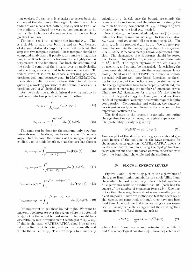
The next step is to calculate the integral vnm. Thisis a double integral over both x1 and x2, but becauseof its computational complexity it is best to break thisstep into two integrals instead. These integrals should becomputed analytically if possible, as numeric integrationmight result in large errors because of the highly oscilla-tory nature of the functions. For both the stadium andthe circle, I computed the integral over x2 analytically,but the integral over x1 had to be done numerically. Toreduce error, it is best to choose a working precision,precision goal, and accuracy goal. In MATHEMATICA,I was able to eliminate errors from this integral by re-questing a working precision of 30 decimal places and aprecision goal of 20 decimal places.

For the circle, the analytic integral over x2 had to bebroken up into two pieces, a top and a bottom:

vx2,top =

∫ 1

√1−x2

1

φm(r)φn(r), (14)

vx2,bottom =

∫ √1−x21

−1

φm(r)φn(r). (15)

The same can be done for the stadium, only now fourintegrals need to be done, one for each corner of the rect-angle. In this case, the bounds of the integral dependexplicitly on the side length a1 that the user has chosen:

vx2,topleft =

∫ 1

√1−(x1+( a1

2 −1))2φm(r)φn(r), (16)

vx2,topright =

∫ 1

√1−(x1−( a1

2 −1))2φm(r)φn(r), (17)

vx2,bottomleft =

∫ −√1−(x1+( a12 −1))2

−1

φm(r)φn(r), (18)

vx2,bottomright =

∫ −√1−(x1−( a12 −1))2

−1

φm(r)φn(r). (19)

It’s important to get these bounds right. We want tomake sure to integrate over the region where the potentialis V0, not in the actual billiard region. There might be adiscontinuity in the evaluation of the integral at n2 = m2.If this is the case, MATHEMATICA should be able totake the limit at this point, and you can manually addit into the value for vx2

. The next step is to numerically

calculate vx1 . In this case the bounds are simply thebounds of the rectangle, and the integrand is simply thesolution to the x2 component of vnm. Computing thisintegral gives us the final vnm needed.

Now that vnm has been calculated, we use (10) to cal-culate the Hamiltonian matrix Hnm. In this calculationn1, n2,m1, and m2 should all run from one to M0. Theterm δnm is the product δm1,n1

δm2,n2. We are now pre-

pared to compute the energy eigenvalues of the system.MATHEMATICA conveniently has an ’eigenvalues’ func-tion. The eigenvalues that it returns should be sortedfrom lowest to highest for proper analysis, and have unitsof ~2/2Ma2

1. The higher eigenvalues are less likely tobe accurate, and so may be discarded. Nonetheless, thelower ones should approximate the actual energy levelsclosely. Solutions to the TISWE for a circular infinitepotential well are well know bessel functions, so check-ing for accuracy of the method should be simple. Whenthe energy eigenvalues have been properly calculated, onecan consider increasing the number of expansion terms.There are M2

0 eigenvalues for a given M0 that can bereturned. A good energy level analysis could use thou-sands of eigenvalues, although this would require lengthycomputation. Computating and ordering the eigenvec-tors is just as easily accomplished, and correspond to theexpansion coefficients cm.

The final step in the program is actually computingthe eigenfunctions ψn(r) using the original expansion (4).The probability density is given by

|ψn(r)|2 = ψn(r)ψn(r). (20)

Doing a plot of this density with a grayscale should givegood images of the solutions to the wave equation forthe geometries in question. MATHEMATICA allows usto draw on top of our plots using the ’epilog’ function,so we can outline the boundaries we were concerned withfrom the beginning (the circle and the stadium).

IV. PLOTS & ENERGY LEVELS

Figures 2 and 3 show a log plot of the eigenvalues ofthe n x m Hamiltonian matrix for the circle billiard andthe stadium billiard respectively. The circle billiards have81 eigenvalues while the stadium has 100 (each has thesquare of the number of expansion terms M0). One maynotice that the energy levels shoot up exponentially aftera certain point. There are methods to test the accuracy ofthe eigenvalues computed, although they have not beenused here. One such method involves using a transforma-tion to linearly scale the energies and then testing theiragreement with a Weyl-formula, such as

〈N(E)〉 =1

4π(AE − L

√E + C) (21)

where A and L are the area and perimeter of the billiard,and C is a topological constant [5]. I have neglected such

4

a test, although it should be done if time is available.I decided to toss the higher energy levels given due tosuspicion about mounting error. Figures 4 and 5 showa selection of density plots of the wavefunctions |ψn| foreach of the systems. The first nine eigenfunctions areshown for the circle, while nine increasing but not con-tinuous eigenfunctions were chosen for the stadium.

FIG. 2: List of eigenvalues for the circle system, generatedusing twenty expansion terms. The higher eigenvalues (n >250) may have been subject to larger numerical roundoff er-rors, and can be discounted from analysis.

FIG. 3: List of eigenvalues for the stadium system, generatedusing twenty expansion terms. Like the circle system, onlythe lower eigenvalues (n < 350) may be trusted in analysis.

V. PRELIMINARY ENERGY SPACINGANALYSIS AND FUTURE WORK

Because quantum mechanical systems do not havephase spaces which can display extreme sensitivity toinitial conditions (as classical systems do), analogues toclassical chaos are sought in the spacing of the energylevels. The energy levels are given by the eigenvalues ofthe Hamiltonian matrix Hnm. One common way to ana-lyze energy level spacings is through a nearest neighborplot. If we have n useable energy levels, then we can ex-amine the spacing between subsequent levels by plottinga normalized histogram of En+1−En about some spacing

FIG. 4: The first nine eigenfunctions of the infinite circu-lar well. These solutions represent the classic bessel functionswhich have historically been used to solve the Helmholtz equa-tion.

FIG. 5: A mixed assortment of eigenfunctions from the sta-dium with horizontal extension a1 = 8.88, with aspect ratioset to one.

ds: ∫P (s)ds =

∑n

En+1 − En

n= 1. (22)

The difference between integrable systems (like the cir-cle) and nonintegrable systems (like the stadium) is thatan integrable system has the same number of constants ofmotion as its dimension, whereas a nonintegrable systemhas fewer constants of motion than its dimension (thoughthat distinction has been contested [6]). According toRandom Matrix Theory, a classically integrable system

5

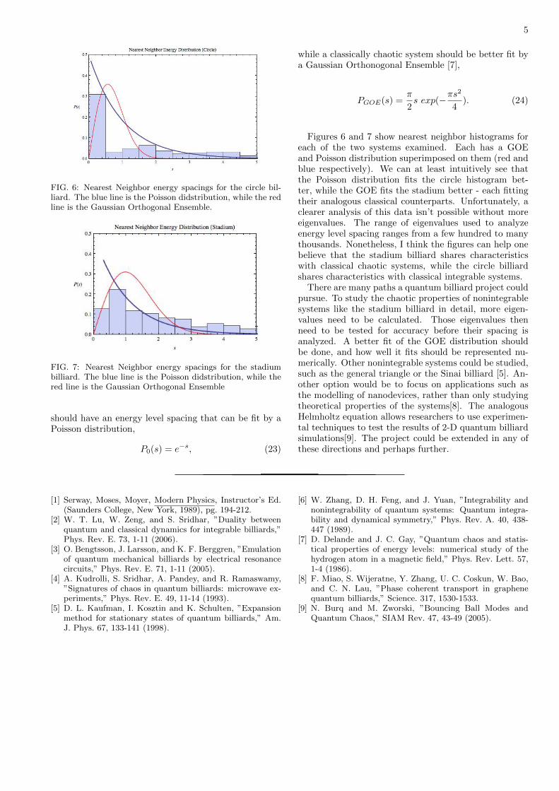
FIG. 6: Nearest Neighbor energy spacings for the circle bil-liard. The blue line is the Poisson didstribution, while the redline is the Gaussian Orthogonal Ensemble.

FIG. 7: Nearest Neighbor energy spacings for the stadiumbilliard. The blue line is the Poisson didstribution, while thered line is the Gaussian Orthogonal Ensemble

should have an energy level spacing that can be fit by aPoisson distribution,

P0(s) = e−s, (23)

while a classically chaotic system should be better fit bya Gaussian Orthonogonal Ensemble [7],

PGOE(s) =π

2s exp(−πs

2

4). (24)

Figures 6 and 7 show nearest neighbor histograms foreach of the two systems examined. Each has a GOEand Poisson distribution superimposed on them (red andblue respectively). We can at least intuitively see thatthe Poisson distribution fits the circle histogram bet-ter, while the GOE fits the stadium better - each fittingtheir analogous classical counterparts. Unfortunately, aclearer analysis of this data isn’t possible without moreeigenvalues. The range of eigenvalues used to analyzeenergy level spacing ranges from a few hundred to manythousands. Nonetheless, I think the figures can help onebelieve that the stadium billiard shares characteristicswith classical chaotic systems, while the circle billiardshares characteristics with classical integrable systems.

There are many paths a quantum billiard project couldpursue. To study the chaotic properties of nonintegrablesystems like the stadium billiard in detail, more eigen-values need to be calculated. Those eigenvalues thenneed to be tested for accuracy before their spacing isanalyzed. A better fit of the GOE distribution shouldbe done, and how well it fits should be represented nu-merically. Other nonintegrable systems could be studied,such as the general triangle or the Sinai billiard [5]. An-other option would be to focus on applications such asthe modelling of nanodevices, rather than only studyingtheoretical properties of the systems[8]. The analogousHelmholtz equation allows researchers to use experimen-tal techniques to test the results of 2-D quantum billiardsimulations[9]. The project could be extended in any ofthese directions and perhaps further.

[1] Serway, Moses, Moyer, Modern Physics, Instructor’s Ed.(Saunders College, New York, 1989), pg. 194-212.

[2] W. T. Lu, W. Zeng, and S. Sridhar, ”Duality betweenquantum and classical dynamics for integrable billiards,”Phys. Rev. E. 73, 1-11 (2006).

[3] O. Bengtsson, J. Larsson, and K. F. Berggren, ”Emulationof quantum mechanical billiards by electrical resonancecircuits,” Phys. Rev. E. 71, 1-11 (2005).

[4] A. Kudrolli, S. Sridhar, A. Pandey, and R. Ramaswamy,”Signatures of chaos in quantum billiards: microwave ex-periments,” Phys. Rev. E. 49, 11-14 (1993).

[5] D. L. Kaufman, I. Kosztin and K. Schulten, ”Expansionmethod for stationary states of quantum billiards,” Am.J. Phys. 67, 133-141 (1998).

[6] W. Zhang, D. H. Feng, and J. Yuan, ”Integrability andnonintegrability of quantum systems: Quantum integra-bility and dynamical symmetry,” Phys. Rev. A. 40, 438-447 (1989).

[7] D. Delande and J. C. Gay, ”Quantum chaos and statis-tical properties of energy levels: numerical study of thehydrogen atom in a magnetic field,” Phys. Rev. Lett. 57,1-4 (1986).

[8] F. Miao, S. Wijeratne, Y. Zhang, U. C. Coskun, W. Bao,and C. N. Lau, ”Phase coherent transport in graphenequantum billiards,” Science. 317, 1530-1533.

[9] N. Burq and M. Zworski, ”Bouncing Ball Modes andQuantum Chaos,” SIAM Rev. 47, 43-49 (2005).