chaos in microwave resonators

Seminaire Poincare IX (2006) 1 – 40 Seminaire Poincare

Chaos in Microwave resonators

Hans-Jurgen StockmannFachbereich Physik der Philipps-Universitat MarburgRenthof 5D-35032 Marburg, Germany

1 Introduction

Up to about 1990 the quantum mechanics of classically chaotic systems, shortlytermed ‘quantum chaos’, was essentially a domain of theory [1]. Only two classes ofexperimental result had been available at that time. First, there were the spectra ofcompound nuclei giving rise to the development of random matrix theory in the sixtiesof the last century, and second the experiments with highly excited hydrogen and alkaliatoms in strong magnetic or strong radio frequency fields. The situation changed withthe appearance of the various types of billiard experiments. After the first microwavestudy performed in the author’s group [2] there were numerous experiments withclassical waves on liquid surfaces, in plates, solids, and rods, with electrons in quantumdots, tunnelling barriers and quantum corrals, and with ultra-cold atoms confined inbilliards formed by light walls. References and a more detailed account on the subjectmay be found in Ref. [3]. It will become clear in the following that the differencebetween classical waves and matter waves is not of relevance, since the universalfeatures we shall discuss are common to all types of wave not necessarily quantummechanically in origin. This is why ‘wave chaos’ would be a better term to describethis field of research, and there are authors avoiding the term ‘quantum chaos’ as awhole.

This article is organized as follows. After a short introduction into the subjectin Section 2, concentrating on the inherent difficulties with the definition of chaosin quantum mechanics, in Section 3 the microwave technique is introduced. In thesubsequent three sections various aspects of quantum chaos are presented and illus-trated by experimental results. The selection was exclusively guided by the intensionto provide experimental illustrations of essential theoretical results. There was not theintent to give an exhaustive overview on the subject. In Section 4 a short introductioninto the concept of random matrices is given, illustrating the remarkable observationthat a mayor part of the statistical properties of the spectra of chaotic systems canbe obtained already if the underlying Hamiltonian is substituted by a matrix theelements of which are chosen at random, only obeying some constraints. In Section5 universal features of the wave functions of chaotic billiards are discussed. Here alot of exact results can be obtained from the simple assumption that at each pointin the billiard the wave function may be looked upon as a superposition of waves,with the same modulus of the wave vector, entering randomly from all directions. InSection 6, semiclassical quantum mechanics is introduced, based on the disseminatingpapers by M. Gutzwiller, establishing a link between the quantum-mechanical Greenfunction and the classical trajectories. The article ends with a presentation of recentapplications of wave-chaos research.

2 T. Damour Seminaire Poincare

(a) (b)

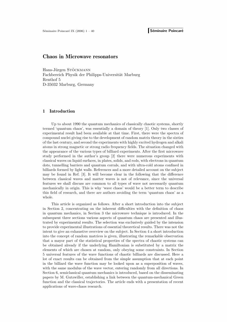
Figure 1 – Classical trajectories in a circular (a) and a stadium (b) billiard.

2 From classical to quantum mechanics

To illustrate the difficulties one is facing with the concept of chaos in quantummechanics, let us first consider an idealised billiard system, i. e. the classical dynamicsof a single particle travelling frictionless through a box with infinitely high walls. Fora circular billiard the trajectory is regular (see Fig. 1(a)). There are two constantsof motion, the total energy E, and the angular momentum L. Since there are twodegrees of freedom as well, the system is integrable. Small uncertainties in the initialconditions, such as the distance between two neighbouring trajectories, will thereforeincrease only linearly in time. The situation is qualitatively different for the stadiumbilliard, the guinea pig in billiard research (see Fig. 1(b)). There is only one constantof motion left, the total energy E, and the distance between neighbouring trajectoriesincreases exponentially with time. The stadium billiard thus is chaotic.

In quantum mechanics this distinction between integrable and chaotic systemsdoes not work. The initial conditions are defined only within the limits of the uncer-tainty relation

∆x∆p ≤ 12~ , (1)

and the concept of trajectories looses its significance. One may even ask whetherquantum chaos does exist at all. Since the Schrodinger equation is linear, a quantummechanical wave packet can be constructed from the eigenfunctions by the superpo-sition principle. But if the wave packet once has been generated, its evolution forarbitrarily long times is available without any problem. There is no room left forchaos.

On the other hand the correspondence principle demands that there must be arelation between linear quantum mechanics and nonlinear classical mechanics at leastin the regime of large quantum numbers. This apparent contradiction has been resol-ved by semiclassical quantum mechanics, derived in essential parts by M. Gutzwillerin a series of papers (see Ref. [4] for a review). The theory relates classical trajectoriesto quantum mechanical spectra and wave functions, and this defines the program ofquantum chaos research, namely to look for the fingerprints of classical chaos in thequantum mechanical properties of the system.

Billiards are ideally suited systems for this purpose. The numerical calculationof the classical trajectories is elementary, and the stationary Schrodinger equationreduces to a simple wave equation

− ~2

2m

(∂2

∂x2+

∂2

∂y2

)ψn = Enψn . (2)

The potential appears only in the boundary condition ψn|S = 0, where S is

Vol. IX, 2006 La Relativite generale aujourd’hui 3

the surface of the billiard. Though billiard systems are conceptually simple, theynevertheless show the full complexity of non-linear systems.

A further advantage is the equivalence of the stationary Schrodinger equationwith the time-independent wave equation, the Helmholtz equation

−(

∂2

∂x2+

∂2

∂y2

)ψn = k2

nψn , (3)

where ψn now is the amplitude of the wave field.

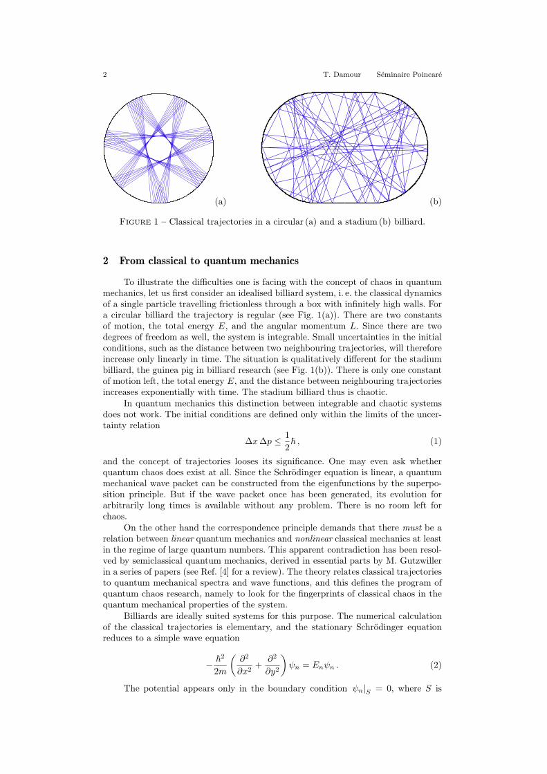
Figure 2 – Chladni giving a public demonstration of his sound figures.

The equivalence of the stationary Schrodinger equation and the Helmholtz equa-tion opens the opportunity to study questions and to test theories, originally moti-vated by quantum mechanics, by means of classical waves. The boundary conditionsfor the classical and the corresponding quantum mechanical systems may differ, butthis is not of relevance for the questions to be treated in this article.

The first experiment of this type dates back already more then 200 years. At theend of the 18th century E. Chladni developed a technique “to make sound visible”,by decorating the nodal lines of vibrating plates with grains of sand. Chladni neverachieved to get a permanent position at an university and earned his livings by givingdemonstrations of his experiments to the public [5]. Figure 2 gives an example. Onoccasion of a stay in Paris 1808, he got an invitation by Napoleon to give a privateperformance in the Tuileries [6]. There is a very vivid report by Chladni on this visit[7] :


“When I entered, he welcomed me, standing in the centre of the room, withthe expressions of his favour. Napoleon showed much interest in my experiments andexplanations and asked me, as an expert in mathematical questions, to explain alltopics thoroughly, so that I could not take the matter too easy. He was well informedthat one is not yet able to apply a calculation to irregularly shaped areas, and that, ifone were successful in this respect, it could be useful for applications to other subjectsas well.”

The last remark had been really visionary ! Who could have imagined at thattime that Chladni’s experiments in a sense mean the starting point of quantum chaosresearch ?

3 Microwave billiards

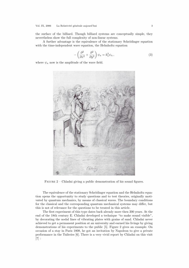
Modern experimental billiard studies started with microwave resonators [2].Fig. 3(left) shows a typical set-up. The cavity is formed by a bottom plate sup-porting the entrance antenna, and by an upper part whose position can be movedwith respect to the lower one. As long as a maximum frequency νmax = c/2d is notexceeded, where d is the height of the resonator and c the velocity of light, the systemcan be considered as quasi-two-dimensional. In this situation the electro-magneticwave equations reduce to the scalar Helmholtz equation (3), where ψn correspondsto the electric field pointing perpendicularly from the bottom to the top plate. Sincethe electric field component parallel to the wall must vanish, we have the conditionψn|S = 0 on the outer circumference S of the resonator. We have thus arrived at acomplete equivalence between a two-dimensional quantum billiard and the correspon-ding quasi-two-dimensional microwave resonator, including the boundary conditions.As an example Fig. 3(right) shows the reflection spectrum of a microwave resonatorof the shape of a quarter stadium [2]. Each minimum in the reflection corresponds toan eigenfrequency of the resonator.

Figure 3 – Microwave set-up to study spectra and wave functions (left), and a typicalmicrowave reflection spectrum (right) [2].

A detailed consideration shows that the measurement directly yields the compo-nents of the scattering matrix S, where the diagonal element Snn corresponds to thereflection amplitude at the nth antenna, and the off-diagonal matrix element Snm tothe transmission amplitude between antennas n and m. For isolated resonances thecomponents of the scattering matrix are given by

Sij(~ri, ~rj , k) = δij − 2ıγ∑

n

ψ∗n(~ri)ψn(~rj)k2 − k2

n + ıΓn, (4)

where kn and ψn(~ri) are the nth k-eigenvalue and eigenfunction at the position ofantenna i. The bar denotes that both quantities are slightly changed as compared


to the closed system. γ is a factor describing the antenna coupling, assumed to beequal for all antennas for the sake of simplicity. In addition the resonances acquirea line width Γn. Apart from these modifications the microwave measurement yieldsdirectly the Green function of the system, and thus the complete quantum mechanicalinformation. Eq. (4) is the quantum-mechanical expression of the scattering matrix.The electromagnetical line widths γn are related to the Γn by Γn = kγn [8]. This isa consequence of the different dispersion relations ω ∼ k and ω ∼ k2 for the electro-magnetic and the quantum-mechanical case, respectively.

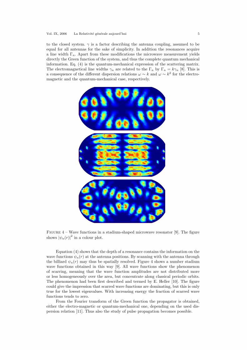
Figure 4 – Wave functions in a stadium-shaped microwave resonator [9]. The figureshows |ψn(r)|2 in a colour plot.

Equation (4) shows that the depth of a resonance contains the information on thewave functions ψn(r) at the antenna positions. By scanning with the antenna throughthe billiard ψn(r) may thus be spatially resolved. Figure 4 shows a number stadiumwave functions obtained in this way [9]. All wave functions show the phenomenonof scarring, meaning that the wave function amplitudes are not distributed moreor less homogeneously over the area, but concentrate along classical periodic orbits.The phenomenon had been first described and termed by E. Heller [10]. The figurecould give the impression that scarred wave functions are dominating, but this is onlytrue for the lowest eigenvalues. With increasing energy the fraction of scarred wavefunctions tends to zero.

From the Fourier transform of the Green function the propagator is obtained,either the electro-magnetic or quantum-mechanical one, depending on the used dis-persion relation [11]. Thus also the study of pulse propagation becomes possible.


Microwave billiards have a number of advantages as compared to nuclei : (a) ty-pical wave lengths are of the order of mm to cm, resulting in very convenient sizes forthe used resonators, (b) shapes of the resonators, coupling strengths to antennas etc.can be perfectly controlled, (c) parameter variations, e. g. of the coupling strength,the position of an impurity, or of one length can be easily achieved, and (d) last butnot least, we have seen that in microwave systems the complete scattering matrixis obtainable, including the phases. This is extraordinary, in standard scattering ex-periments, such as in in nuclear physics, usually only reduced information, such asscattering cross-sections, is available, resulting in a complete loss of the phase infor-mation. This is why a number of predictions of scattering theory have been testednot in nuclei but microwave billiards.

4 Random Matrices

In the spring times of nuclear physics in the midst of the last century there ap-peared a vast amount of experimental results on cross-sections, partial cross-sectionetc., obtained by bombarding target nuclei with light projectiles. Nearly nothing wasknown at that time on the origin of the nuclear forces. Could it be expected undersuch circumstances to obtain any relevant information at all from these irregularlylooking spectra without any recognisable pattern ? Here one idea showed up to beextremely useful, notwithstanding its obviously oversimplifying nature : If nothing isknown on the nuclear Hamiltonian H, just let us take its matrix elements in some basisas random numbers, with only some global constraints, e. g. by taking the matrix Hsymmetric for systems with, or Hermitian for systems without time-reversal symme-try, and by fixing the variance of its matrix elements. Assuming basis invariance of thedistribution of the matrix elements one immediately sees that the matrix elements areuncorrelated and Gaussian distributed [12]. There are three Gaussian ensembles, theorthogonal one (GOE) for time-reversal invariant systems with integer spin, the uni-tary one (GUE) for systems with broken time-reversal symmetry, and the symplecticone (GSE) for time-reversal invariant systems with half-integer spin. Here ‘orthogo-nal’ etc. refers to the invariance properties of the respective ensembles. Recently it hasbeen shown by M. Zirnhauer [13] that in fact there are seven additional ensembles,which become relevant, whenever pair-wise creation and annihilation of particles isinvolved, as it is the case in elementary particle physics and superconductivity. For allGaussian ensembles exact expressions for many quantities of interest can be calcula-ted explicitly, such as spectral correlation functions, eigenvalue spacings distributionsetc. .

The quantity most often studied in this context is the distribution of level spa-cings p(s) normalised to a mean level spacing of one. For 2× 2 matrices this quantitycan be easily calculated, yielding for the GOE the famous Wigner surmise

p(s) =π

2s exp

(−π

4s2

). (5)

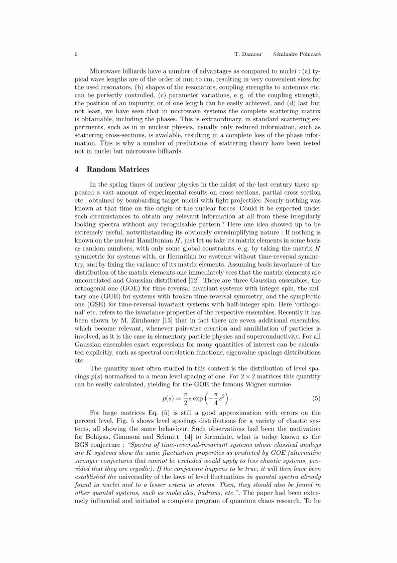
For large matrices Eq. (5) is still a good approximation with errors on thepercent level. Fig. 5 shows level spacings distributions for a variety of chaotic sys-tems, all showing the same behaviour. Such observations had been the motivationfor Bohigas, Giannoni and Schmitt [14] to formulate, what is today known as theBGS conjecture : “Spectra of time-reversal-invariant systems whose classical analogsare K systems show the same fluctuation properties as predicted by GOE (alternativestronger conjectures that cannot be excluded would apply to less chaotic systems, pro-vided that they are ergodic). If the conjecture happens to be true, it will then have beenestablished the universality of the laws of level fluctuations in quantal spectra alreadyfound in nuclei and to a lesser extent in atoms. Then, they should also be found inother quantal systems, such as molecules, hadrons, etc.”. The paper had been extre-mely influential and initiated a complete program of quantum chaos research. To be


Figure 5 – Level spacing distribution for a Sinai billiard (a), a hydrogen atom in astrong magnetic field (b), the excitation spectrum of a NO2 molecule (c), the acousticresonance spectrum of a Sinai-shaped quartz block (d), the microwave spectrum of athree-dimensional chaotic cavity (e), and the vibration spectrum of a quarter-stadiumshaped plate (f) (taken from Ref. [3]). In all cases a Wigner distribution is foundthough only in the first three cases the spectra are quantum mechanically in origin.

fair one should mention that there had been another paper on the same subject [15]somewhat earlier, which, however, at that time did not find the attendance it wouldhave deserved.

The replacement of H by a random matrix means to abandon any hope to learnmore about nuclei from the spectra but some average quantities such as the mean levelspacings. Of course this is not the end of the story : there are techniques to extractalso individual system properties. We shall come back to this aspect in Section 6. Butthe loss of individual features in the spectra on the other hand means that it might beworthwhile to look for universal features being common to all chaotic systems. Thisapproach showed up to be extremely fruitful. It allowed to apply results originallyobtained for nuclei to many other systems as well, in particular quantum-dot systems[16] and microwave billiards [3].

In addition to the level spacings distribution in particular spectral correlations


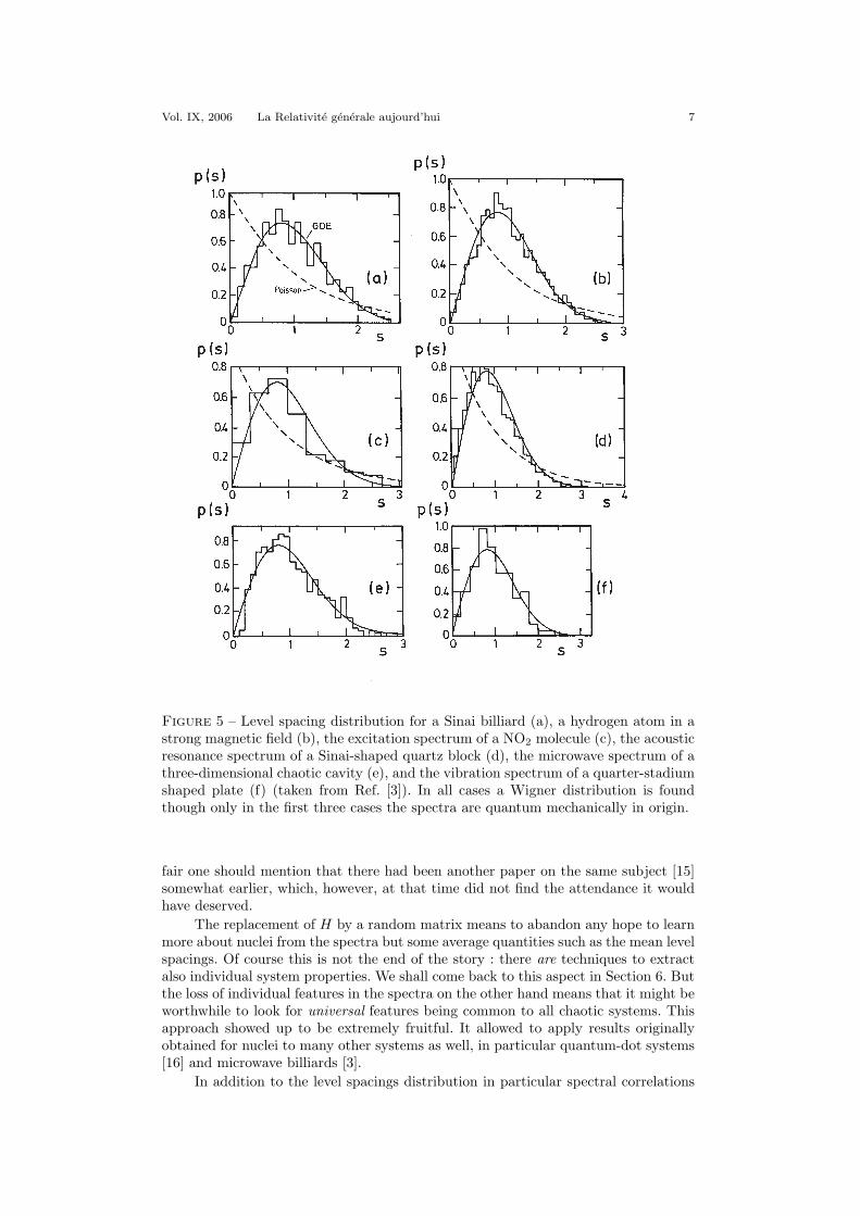
Figure 6 – Spectral form factor for the spectrum of a microwave hyperbola billiard(top), and for the subspectrum obtained by considering only every second resonance(bottom) [17].

related to the spectral auto-correlation function C(E) = 〈ρ(E2)ρ(E1)〉−〈ρ(E2)〉〈ρ(E1)〉are considered, where E = E2−E1, and the brackets denote a spectral average. Quan-tities often studied in literature are number variance and spectral rigidity, see e. g.Ref. [3] for details. Here another object shall be considered, the spectral form factorK(t), since it will be of importance for the understanding of the relation betweenrandom matrix theory and semiclassical quantum mechanics to be discussed in Sec-tion 6. K(t) is obtained from the Fourier transform of the spectral auto-correlationfunction. Random matrix theory yields explicit expressions. For later use the resultsfor the GOE and the GUE shall be given (see e. g. Ref. [1]) :

KGOE(t) ={

2t− t ln(1 + 2t)2− t ln 2t+1

2t−1

, KGUE(t) ={

t t < 11 t > 1 . (6)

The time is given in units of the Heisenberg time tH = ~/〈∆E〉, where 〈∆E〉 isthe mean level spacings.

Fig. 6 shows as an experimental example the spectral form factor for a hyperbolabilliard obtained in the group of A. Richter [17]. In the upper part of the figureK(t) for the complete spectrum is shown. There is a good agreement with randommatrix predictions from the GOE. This is consistent with the fact that microwavebilliard systems are time-reversal invariant, and there is no spin. Spectra showingGSE statistics have not yet been studied experimentally, but there is the remarkablefact that GSE spectra can be generated by taking only every second level of a GOEspectrum [12]. Exactly this had been dome with the spectrum of the hyperbola billiardto obtain the spectral form factor in the lower part of the figure, being in perfectagreement with the expected GSE behaviour.


5 The random plane wave approximation

In a disseminating paper on wave functions in the stadium billiard McDonaldand Kaufman noticed [18] that for most wave functions the amplitudes ψ are Gaussiandistributed,

Pψ(ψ) =

√A

2πexp

(−Aψ2

2

), (7)

where A is the billiard area. Exceptions are scarred wave functions of the type shownin Fig. 4. For the intensities ρ = |ψ|2 of the wave function follows a Porter-Thomasdistribution,

Pρ(ρ) =

√A

2πρexp

(−Aρ

2

). (8)

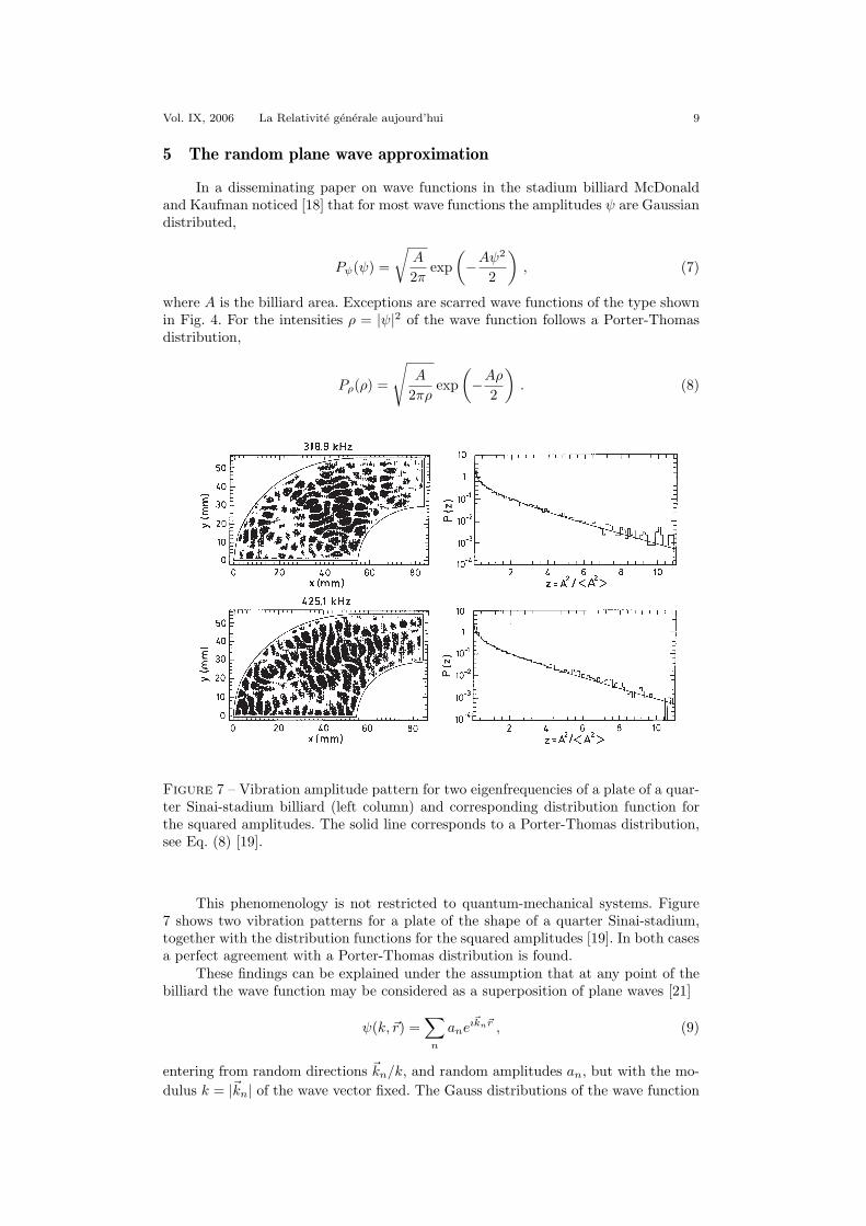
Figure 7 – Vibration amplitude pattern for two eigenfrequencies of a plate of a quar-ter Sinai-stadium billiard (left column) and corresponding distribution function forthe squared amplitudes. The solid line corresponds to a Porter-Thomas distribution,see Eq. (8) [19].

This phenomenology is not restricted to quantum-mechanical systems. Figure7 shows two vibration patterns for a plate of the shape of a quarter Sinai-stadium,together with the distribution functions for the squared amplitudes [19]. In both casesa perfect agreement with a Porter-Thomas distribution is found.

These findings can be explained under the assumption that at any point of thebilliard the wave function may be considered as a superposition of plane waves [21]

ψ(k, ~r) =∑

n

aneı~kn~r , (9)

entering from random directions ~kn/k, and random amplitudes an, but with the mo-dulus k = |~kn| of the wave vector fixed. The Gauss distributions of the wave function


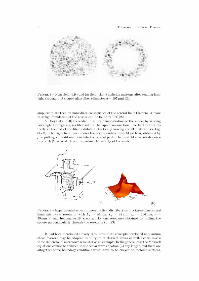
Figure 8 – Near-field (left) and far-field (right) emission patterns after sending laserlight through a D-shaped glass fiber (diameter d = 107 µm) [20].

amplitudes are then an immediate consequence of the central limit theorem. A morethorough foundation of the ansatz can be found in Ref. [22].

V. Doya et al. [20] succeeded in a nice demonstration of the model by sendinglaser light through a glass fiber with a D-shaped cross-section. The light output di-rectly at the end of the fiber exhibits a chaotically looking speckle pattern, see Fig.8(left). The right hand part shows the corresponding far-field pattern, obtained byjust putting an additional lens into the optical path. The far-field concentrates on aring with |k| =const., thus illustrating the validity of the model.

(a) (b)

Figure 9 – Experimental set-up to measure field distributions in a three-dimensionalSinai microwave resonator with Lx = 96mm, Ly = 82 mm, Lz = 106 mm, r =39mm (a) and frequency-shift spectrum for one resonance obtained by pulling thesphere perpendicularly through the resonator (b) [23].

It had been mentioned already that most of the concepts developed in quantumchaos research may be adopted to all types of classical waves as well. Let us take athree-dimensional microwave resonator as an example. In the general case the Maxwellequations cannot be reduced to the scalar wave equation (3) any longer, and there arealtogether three boundary conditions which have to be obeyed on metallic surfaces,


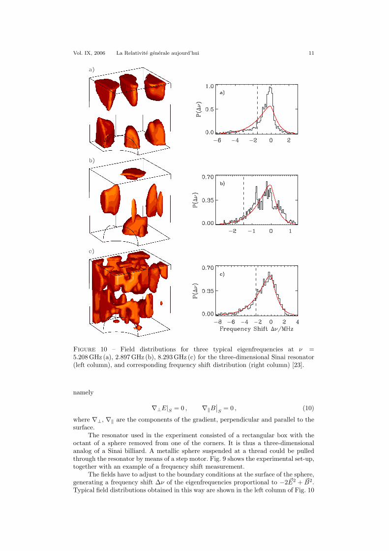
Figure 10 – Field distributions for three typical eigenfrequencies at ν =5.208GHz (a), 2.897 GHz (b), 8.293 GHz (c) for the three-dimensional Sinai resonator(left column), and corresponding frequency shift distribution (right column) [23].

namely

∇⊥E|S = 0 , ∇‖B∣∣S

= 0 , (10)

where ∇⊥, ∇‖ are the components of the gradient, perpendicular and parallel to thesurface.

The resonator used in the experiment consisted of a rectangular box with theoctant of a sphere removed from one of the corners. It is thus a three-dimensionalanalog of a Sinai billiard. A metallic sphere suspended at a thread could be pulledthrough the resonator by means of a step motor. Fig. 9 shows the experimental set-up,together with an example of a frequency shift measurement.

The fields have to adjust to the boundary conditions at the surface of the sphere,generating a frequency shift ∆ν of the eigenfrequencies proportional to −2 ~E2 + ~B2.Typical field distributions obtained in this way are shown in the left column of Fig. 10


[23]. To visualise the distributions, a surface of constant frequency shift, i. e. of aconstant value of −2 ~E2 + ~B2, has been shaded. The examples shown allow an easyinterpretation. The field distribution in the upper panel corresponds to a standingwave between the vertical planes, whereas the field distribution shown in the centralrow is scarred along a periodic orbit of the shape of a diamond. Finally, the fielddistribution in the bottom panel has a completely chaotic appearance.

To substantiate these observations, on the right column of Fig. 10 the distribu-tions of frequency shifts ∆ν ∼ −2 ~E2 + ~B2 are plotted. Under the assumption thatall six field components Ex, . . ., Bz are uncorrelated and Gaussian distributed, thefrequency shift distribution function can be calculated. The result is the solid line.A perfect agreement with the experiment is found for the chaotically looking fielddistribution of Fig. 10(c), whereas for the two other examples the solid line is notable to describe the experimental findings.

What does this mean ? At first sight the assumption of uncorrelated field com-ponents seems to be very strong. After all the components of ~E and ~B are intimatelylinked via the Maxwell equations. But if we assume again that the chaotic field dis-tribution can be obtained by a superposition of plane waves, now of electromagneticwaves, the correlations disappear and one ends up exactly with the applied modelof uncorrelated Gaussian distributed field components. The same model which hadbeen applied with great success to quantum billiards, thus does work equally well forelectromagnetic systems.

6 Semiclassical quantum mechanics

Before quantum mechanics had been established in its present form by Heisen-berg, Schrodinger and others, it had been Bohr, and later Born and Sommerfeld,who developed a technique today known as semi-classical to calculate the spectrumof atomic hydrogen. At that time Einstein [24] argued that this approach must bea dead end, since semi-classical quantisation needs invariant tori in the phase space,preventing a semi-classical quantisation for non-integrable systems. This would meanthat the technique applied hitherto would work for hydrogen-like systems only, sincealready the second element in the periodic system, Helium, is non-integrable. Thishad been one of the rare cases, where Einstein was wrong, though it needed half acentury until M. Gutzwiller [4] showed in a series of papers that chaotic systems, too,allow for a semi-classical quantisation.

Starting point of his approach is Feynman’s path integral for the quantum-mechanical propagator

K(qA, qB , t) =∫D(q)W (q) exp

[ı

~

∫ t

0

L(q, q) dt

], (11)

giving the probability amplitude for a particle to propagate in time t from qA to qB .The expression on the right hand side means in a symbolical short-hand notation anintegral over all pathes, classically allowed or forbidden, from qA to qB , where W (q)takes into account the stability of the trajectory, and L(q, q) is the Lagrange function.It is remarkable that both quantities are purely classical, quantum mechanics enteringonly via the 1/~ in the exponential. Expression (11) is not particulary useful for anexplicit calculation of the propagator, since it involves a multi-dimensional integral,but it is very well suited as a starting point for a semi-classical approach.

In the semiclassical limit the phase factors are strongly fluctuating quantities,and only terms contribute significantly, where the phase is stationary, i. e. where thecondition

δ

∫L(q, q, t)dt = 0 (12)


is met, where the variation is over all paths connecting qA and qB . But this is exactlyHamilton’s principle of classical mechanics, from which the classical equations of mo-tion can be derived. Expressed in other words : In the semi-classical limit only theclassically allowed paths contribute to the path integral (11) !

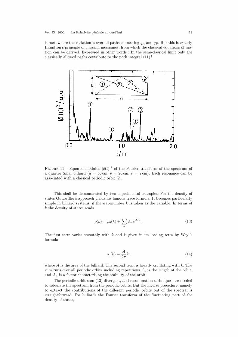
Figure 11 – Squared modulus |ρ(t)|2 of the Fourier transform of the spectrum ofa quarter Sinai billiard (a = 56 cm, b = 20 cm, r = 7 cm). Each resonance can beassociated with a classical periodic orbit [2].

This shall be demonstrated by two experimental examples. For the density ofstates Gutzwiller’s approach yields his famous trace formula. It becomes particularlysimple in billiard systems, if the wavenumber k is taken as the variable. In terms ofk the density of states reads

ρ(k) = ρ0(k) +∑

n

Aneıkln . (13)

The first term varies smoothly with k and is given in its leading term by Weyl’sformula

ρ0(k) =A

2πk , (14)

where A is the area of the billiard. The second term is heavily oscillating with k. Thesum runs over all periodic orbits including repetitions. ln is the length of the orbit,and An is a factor characterising the stability of the orbit.

The periodic orbit sum (13) divergent, and resummation techniques are neededto calculate the spectrum from the periodic orbits. But the inverse procedure, namelyto extract the contributions of the different periodic orbits out of the spectra, isstraightforward. For billiards the Fourier transform of the fluctuating part of thedensity of states,


ρosc(l) =∫

ρosc(k)e−ıkl dk

=∑

n

Anδ(l − ln) , (15)

directly yields the contributions of the orbits to the spectrum [2]. Each orbit gives riseto a delta peak at an l value corresponding to its length, and a weight correspondingto the stability factor of the orbit.

Figure (11) shows for illustration the squared modulus of the Fourier transformof the spectrum of a microwave resonator shaped as a quarter Sinai billiard [2]. Eachpeak corresponds to a periodic orbit of the billiard. For the bouncing ball orbit,labelled by ©1 , three peaks associated with repeated orbits are clearly visible. Thesmooth part of the density of states is responsible for the increase of |ρ(k)|2 at smalllengths.

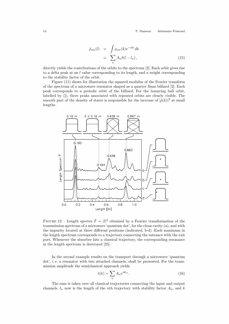
Figure 12 – Length spectra T = |t|2 obtained by a Fourier transformation of thetransmission spectrum of a microwave ‘quantum dot’, for the clean cavity (a), and withthe impurity located at three different positions (indicated, b-d). Each maximum inthe length spectrum corresponds to a trajectory connecting the entrance with the exitport. Whenever the absorber hits a classical trajectory, the corresponding resonancein the length spectrum is destroyed [25].

In the second example results on the transport through a microwave ‘quantumdot’, i. e. a resonator with two attached channels, shall be presented. For the trans-mission amplitude the semiclassical approach yields

t(k) =∑

n

Aneikln . (16)

The sum is taken over all classical trajectories connecting the input and outputchannels. ln now is the length of the nth trajectory with stability factor An, and k


is the wavenumber. By taking the Fourier transform of the transmission, one obtainsagain the stability-weighted length spectrum, allowing for an immediate identificationof the relevant transport pathes :

t(l) =12π

∫t(k)e−ikldk =

∑n

Anδ(l − ln). (17)

In Fig. 12, length spectra T = |t|2, such obtained are presented. For the emptythe cavity (a), the length spectrum shows a number of peaks which can be associatedwith classical trajectories, shown in the upper part of the figure. With an absorberplaced in the cavity, the magnitude of the length peaks depends sensitively on theabsorber position position : whenever the absorber lies close to the semiclassical tra-jectory associated with a particular resonance in the length spectrum, the resonanceis destroyed. If, on the other hand, the absorber misses the trajectory, the resonanceremains intact. With this technique the length peaks can be associated unambiguouslywith the corresponding trajectories.

Semiclassical quantum mechanics relates the spectrum to the classical periodicorbits of the system, i. e. to individual system properties. In view of this fact one maywonder where the universal features discussed in Section 3 come in. To answer thisquestion let us have a look onto the spectral form factor K(t), introduced in Section 3as the Fourier transform of the spectral autocorrelation function. Entering here withthe trace formula, a semiclassical expression for K(t) is obtained, which for billiardsread

K(t) =∑n,m

A∗nAmδ [t− (tn + tm)/2] eık(ln−lm)t . (18)

K(t) shows peaks at times (tn + tm)/2, where tn = ln/c is the period for the nthorbit. For short times all these peaks are well-separated. It is essentially this what isseen in Fig. 11. But with increasing time, because of the exponential proliferation ofthe long orbits in chaotic systems, the density of these peaks becomes so large thatonly an overall increase of K(t) can be observed. This is the onset of the universalregime. In the so-called diagonal approximation it is argued that only terms withn = m contribute, since the off-diagonal contributions are averaged out by the phasefactor eık(ln−lm)t. For systems with time-reversal symmetry one has to consider inaddition that all orbits come in pairs corresponding to clock- and counter-clock-wisepropagation. Under this assumption Eq. (18) yields KGOE = 2t and KGUE = t beingjust the leading terms of the expressions given in Eq. (6) for t < 1. This had beenshown already 30 years ago by M. Berry [26]. It needed 25 more years until it wasrecognised by M. Sieber and K. Richter [27] that there are off-diagonal terms givingnon-negligible contributions. They are associated with pairs of orbits of the topologyof the digit ‘8’, one of them self-intersecting, the other one with an avoided crossinginstead. The corresponding off-diagonal contributions give the next term in the seriesexpansion of K(t). For the GUE this contribution is zero since here the first ordercontribution gives already the exact result (as long as t < 1). The program wascompleted by the Haake group [28] who showed that all orders in the expansioncan be recovered by considering bundles of orbits with more and more crossings andavoided crossings. In a final step they achieved to extend the validity of the approachto times t > 1 [29]. This may be considered as the proof of the BGS conjecture, atleast on the level of the spectral form factor.

7 Applications

Occasionally people doubt whether chaotic systems really need an extra quantum-mechanical treatment. The Schrodinger equation after all gives exact results both for


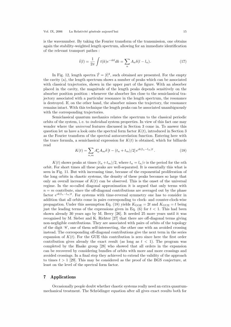
Figure 13 – Snapshot of the pulse propagation in a dielectric quadrupole cavitymade of teflon (length of the long axis l = 113 mm). The left figure shows the pulseintensity inside the teflon at the moment of strongest emission in a colour plot. Inaddition the Poynting vector is shown in the region outside of the teflon. The rightfigure shows the Husimi distribution of the pulse in a Poincare plot. In addition theunstable manifold of the rectangular orbit is shown [30].

regular and chaotic systems. Random matrix theory and the random-plane-wave ap-proach, on the other hand mean caricatures of the true situation, and the semiclassicalapproach at best gives approximate results for high energies. Nowadays the numeri-cal solution of the Schrodinger equation is no challenge any longer even for fairlycomplicated systems. Why should one resort to old-fashioned techniques which hadbeen abandoned already 80 years ago, after the development of ‘correct’ quantummechanics had been been completed ?

First, the semiclassical methods had not been developed as an alternative to theSchrodinger equation to calculate spectra of chaotic systems. This had been successfulin exceptional cases only. And random matrix theory had been devised from the verybeginning as a tool to understand the universal features of the spectra, but obviouslynot to get any information on the individual properties.

But the numerical solution of the Schrodinger equation means a black-box cal-culation, and the human brain is not adopted to perform fast Fourier transforms.This is why spectra as the one shown in Fig. 3 seemingly do not contain any relevantinformation. But the brain is extremely good in identifying pathes and trajectories,and therefore the representation of the spectra in terms of classical trajectories, asshown in Figs. 11 and Fig. 12 allows an immediate suggestive interpretation.

All this is not just l’art pour l’art, as shall be demonstrated by two recentexamples.

The relation between wave propagation and classical trajectories had become ofpractical importance in the development of microlasers. It had been found by Gmachlet al. [31] in quadrupolarly deformed dielectric disks that the strongest emission doesnot occurs at the points of largest curvature. J. Nockel an d D. Stone [32] proposed theclassical phase space properties to be responsible for this at first sight counterintuitivebehaviour. Again this shall be demonstrated by a microwave study. The left partof Fig. 13 shows the snapshot of the pulse propagation in a dielectric quadrupoleresonator made of teflon. The pulse had been generated by a Fourier transform fromthe experimentally determined scattering matrix S12(~r1, ~r2, k), with ~r1 fixed, and ~r2

variable, as described in Section 3. The pulse starts as an outgoing circular wave froman antenna close to the boundary in the lower part of the cavity, but already aftera short time only two pulses survive circulating clock- and counter-clockwise close tothe border. For the figure a moment has been selected where there is a particularly


strong emission to the outside. In the right part of the figure the same situation isshown in a Poincare plot, with the polar angle as the abscissa, and the sine of theincidence angle as the ordinate. In a Poincare plot each trajectory is mapped onto asequence of points representing the reflections at the boundary. The intricate tongue-like structure represents the instable manifold of the rectangle. It had been obtainedby starting a trajectory with a minute deviation from the instable rectangular periodicorbit. In addition the Husimi representation of the pulse in the right hand part of thefigure is shown. A Husimi distribution maybe looked upon as a decomposition od aquantum-mechanical wave function in terms of wave packets of minimum uncertainty,and is a convenient tool to establish a correspondence between wave propagation andclassical trajectories (see e. g. Ref. [33]). Now it becomes obvious why the strongestemission does not occur at the points of strongest emission. Teflon has an indexof refraction of n = 1.44 meaning a sin χcrit = 0.69 for the critical angle of totalreflection. Thus the circulating pulses are trapped by total reflection, apart from aweak tunnelling escape due the curvature of the boundary. But whenever the criticalline of total reflection is surpassed, there is a strong escape. This happens exactly inthe region of the most pronounced tongues of the instable manifold of the rectangularorbit. It is thus this orbit, acting as a dynamical barrier, which is responsible for theobserved emission behaviour [34]. In the following years ‘phase space engineering’ hasbecome an important tool towards the ultimate goal to construct a microcavity withunidirectional emission [35].

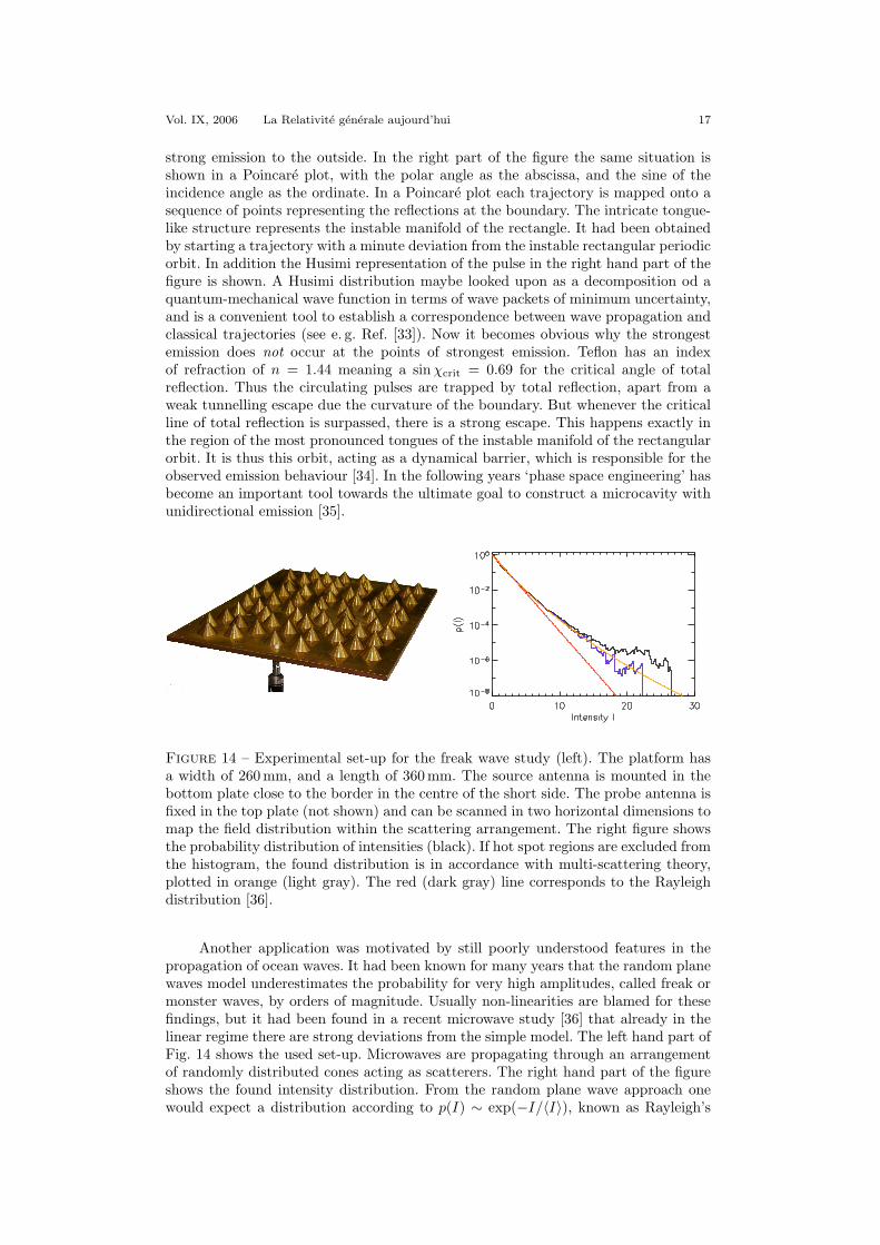
Figure 14 – Experimental set-up for the freak wave study (left). The platform hasa width of 260 mm, and a length of 360 mm. The source antenna is mounted in thebottom plate close to the border in the centre of the short side. The probe antenna isfixed in the top plate (not shown) and can be scanned in two horizontal dimensions tomap the field distribution within the scattering arrangement. The right figure showsthe probability distribution of intensities (black). If hot spot regions are excluded fromthe histogram, the found distribution is in accordance with multi-scattering theory,plotted in orange (light gray). The red (dark gray) line corresponds to the Rayleighdistribution [36].

Another application was motivated by still poorly understood features in thepropagation of ocean waves. It had been known for many years that the random planewaves model underestimates the probability for very high amplitudes, called freak ormonster waves, by orders of magnitude. Usually non-linearities are blamed for thesefindings, but it had been found in a recent microwave study [36] that already in thelinear regime there are strong deviations from the simple model. The left hand part ofFig. 14 shows the used set-up. Microwaves are propagating through an arrangementof randomly distributed cones acting as scatterers. The right hand part of the figureshows the found intensity distribution. From the random plane wave approach onewould expect a distribution according to p(I) ∼ exp(−I/〈I〉), known as Rayleigh’s


Figure 15 – A ‘hot spot’, observed at a frequency of 8.85 GHz. The experimentalprobability density for observing such a hot spot is one to two orders of magnitudelarger than that expected from multiple scattering theory [36].

law. The actually found probability densities for high intensities are larger by ordersof magnitudes. First, there is a multiple scattering correction, which had been knownalready for some time [37]. But in addition there is another contribution which couldbe attributed to the formation of hot spots due to caustics in the potential landscapegenerated by the cones. Figure 15 shows one of these hot spots. Without callinginto question the importance of non-linearities for the generation of freak waves inprinciple, a better understanding of non-random features the linear regime is obviouslyneeded.

The number of activities on the transport of different types of waves, light,seismic waves, water waves, sound waves etc. through disordered media is steadily in-creasing, many of them based on theories and techniques originally developed in waveand quantum chaos. After several decades of basic research the time for applicationshas come.

Most of the experimental examples presented in this article have been performedin the author’s group at the university of Marburg. I want to thank all my coworkersfor their excellent work. In particular I would like to mention my senior coworker U.Kuhl who shared the responsibility for the experiments with me over many years. Theexperiments had been funded by the Deutsche Forschungsgemeinschaft by numerousindividual grants, and during the last three year via the research group 760 “Scatteringsystems with complex dynamics”.

References

[1] F. Haake, Quantum Signatures of Chaos. 2nd edition (Springer, Berlin, 2001).

[2] H.-J. Stockmann and J. Stein, Phys. Rev. Lett. 64, 2215 (1990).

[3] H.-J. Stockmann, Quantum Chaos - An Introduction (University Press, Cam-bridge, 1999).

[4] M. C. Gutzwiller, Chaos in Classical and Quantum Mechanics, InterdisciplinaryApplied Mathematics, Vol. 1 (Springer, New York, 1990).


[5] D. Ullmann, Eur. Phys. J. Special Topics 145, 25 (2007).

[6] H.-J. Stockmann, Eur. Phys. J. Special Topics 145, 15 (2007).

[7] F. Melde, Chladnis’s Leben und Wirken (N. G. Elwert’sche Verlagsbuchhandlung,Marburg, 1888).

[8] U. Kuhl, H.-J. Stockmann, and R. Weaver, J. Phys. A 38, 10433 (2005).

[9] J. Stein and H.-J. Stockmann, Phys. Rev. Lett. 68, 2867 (1992).

[10] E. J. Heller, Phys. Rev. Lett. 53, 1515 (1984).

[11] J. Stein, H.-J. Stockmann, and U. Stoffregen, Phys. Rev. Lett. 75, 53 (1995).

[12] M. L. Mehta, Random Matrices. 2nd edition (Academic Press, San Diego, 1991).

[13] M. R. Zirnbauer, J. Math. Phys. 37, 4986 (1996).

[14] O. Bohigas, M. J. Giannoni, and C. Schmit, Phys. Rev. Lett. 52, 1 (1984).

[15] G. Casati, F. Valz-Gris, and I. Guarnieri, Lett. Nuov. Cim. 28, 279 (1980).

[16] C. W. J. Beenakker, Rev. Mod. Phys. 69, 731 (1997).

[17] H. Alt et al., Phys. Rev. E 55, 6674 (1997).

[18] S. W. McDonald and A. N. Kaufman, Phys. Rev. Lett. 42, 1189 (1979).

[19] K. Schaadt, T. Guhr, C. Ellegaard, and M. Oxborrow, Phys. Rev. E 68, 036205(2003).

[20] V. Doya, O. Legrand, F. Mortessagne, and C. Miniatura, Phys. Rev. Lett. 88,014102 (2002).

[21] M. V. Berry, J. Phys. A 10, 2083 (1977).

[22] S. Hortikar and M. Srednicki, Phys. Rev. Lett. 80, 1646 (1998).

[23] U. Dorr, H.-J. Stockmann, M. Barth, and U. Kuhl, Phys. Rev. Lett. 80, 1030(1998).

[24] A. Einstein, Verhandlungen der Deutschen Physikalischen Gesellschaft 19, 82(1917).

[25] Y.-H. Kim et al., Phys. Rev. B 68, 045315 (2003).

[26] M. V. Berry, Proc. R. Soc. Lond. A 400, 229 (1985).

[27] M. Sieber and K. Richter, Phys. Scr. T90, 128 (2001).

[28] S. Muller et al., Phys. Rev. Lett. 93, 014103 (2004).

[29] S. Heusler et al., Phys. Rev. Lett. 98, 044103 (2007).

[30] R. Schafer, U. Kuhl, and H.-J. Stockmann, New J. of Physics 8, 46 (2006).

[31] C. Gmachl et al., Science 280, 1556 (1998).

[32] J. U. Nockel and A. D. Stone, Nature 385, 45 (1997).

[33] A. Backer, S. Furstberger, and R. Schubert, Phys. Rev. E 70, 036204 (2004).

[34] H. G. L. Schwefel et al., J. Opt. Soc. Am. B 21, 923 (2004).

[35] J. Wiersig and M. Hentschel, Phys. Rev. Lett. 100, 033901 (2008).

[36] R. Hohmann et al., Phys. Rev. Lett. 104, 093901 (2010).

[37] T. M. Nieuwenhuizen and M. C. W. van Rossum, Phys. Rev. Lett. 74, 2674(1995).

chaos in microwave resonators

Documents