channel coding.pdf
TRANSCRIPT
ECE 544 – Digital Communications
Besma SMIDA
Chapter 5
Fall 2014
B. Smida (ECE) ECE 544 Fall 2014 1 / 39
Differential Entropy
Definition:
The differential entropy h(X ) of a continuous random variable X withdensity f (x) is defined as
h(X ) = −∫
S
f (x) log f (x)dx = −E[log f (x)],
where S is the support set of the random variable.
Remember that we use the convention 0 log 0 = 0
B. Smida (ECE) ECE 544 Fall 2014 2 / 39
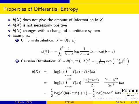
Properties of Differential Entropy
h(X ) does not give the amount of information in X
h(X ) is not necessarily positive
h(X ) changes with a change of coordinate systemExamples:
1 Uniform distribution: X ∼ U(a, b)
h(X ) = −∫ b
a
1
b − alog
1
b − adx = log(b − a)
2 Gaussian Distribution: X ∼ N(µ, σ2), f (x) = 1√2πσ2
exp(
−(x−µ)2
2σ2
)
h(X ) = − log(e)
∫ ∞
−∞
f (x) ln f (x)dx
= − log(e)
∫ ∞
−∞
f (x)(− ln(2πσ2)
2− (x − µ)2
2σ2)dx
=1
2log(e)(ln(2πσ2) + 1) =
1
2log(2πeσ2) bits
B. Smida (ECE) ECE 544 Fall 2014 3 / 39
Two Statements
Consider information transmission over an additive white Gaussiannoise (AWGN) channel. The average transmitted signal power is P ,the noise power spectral density is N0/2 and the bandwidth is W .Two statements are:
1 For each transmission rate rb, there is a corresponding limit on theprobability of bit error one can achieve.
2 For some appropriate signalling rate rb , there is no limit on theprobability of bit error one can achieve, i.e., one can achieve error-freetransmission.
Which statement sounds reasonable to you?
B. Smida (ECE) ECE 544 Fall 2014 4 / 39
Shannon’s Channel Capacity
Shannon proved that it is theoretically possible to transmitinformation at any rate rb, where rb < C , with an arbitrarily smallerror probability by using a sufficiently complicated coding scheme.For rb > C , it is not possible to achieve an arbitrarily small errorprobability.
Shannon’s work showed that the values of P , N0 and W set a limiton transmission rate, not on error probability!
B. Smida (ECE) ECE 544 Fall 2014 5 / 39
Discrete-time Gaussian Channel Capacity
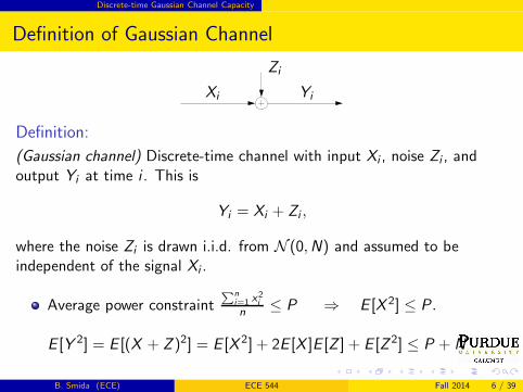
Definition of Gaussian Channel
Xi Yi
Zi
Definition:
(Gaussian channel) Discrete-time channel with input Xi , noise Zi , andoutput Yi at time i . This is
Yi = Xi + Zi ,
where the noise Zi is drawn i.i.d. from N (0,N) and assumed to beindependent of the signal Xi .
Average power constraint∑
n
i=1 x2i
n≤ P ⇒ E [X 2] ≤ P .
E [Y 2] = E [(X + Z )2] = E [X 2] + 2E [X ]E [Z ] + E [Z 2] ≤ P + N
B. Smida (ECE) ECE 544 Fall 2014 6 / 39
Discrete-time Gaussian Channel Capacity
Information Capacity
Definition:
The information capacity with power constraint P is
C = maxE [X 2]≤P
I (X ;Y ).
I (X ;Y ) = h(Y )− h(Y |X ) = h(Y )− h(X + Z |X )
= h(Y )− h(Z |X ) = h(Y )− h(Z )
≤ 1
2log(2πe(P + N)) − 1
2log(2πeN)
=1
2log(1 +
P
N)
The optimum input is Gaussian and the worst noise is Gaussian
B. Smida (ECE) ECE 544 Fall 2014 7 / 39
Discrete-time Gaussian Channel Capacity
Sphere Packing
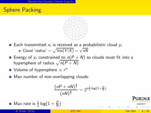
Each transmitted xi is received as a probabilistic cloud yiCloud ’radius’ =
√Var(Y |X ) =
√nN
Energy of yi constrained to n(P + N) so clouds must fit into ahypersphere of radius
√n(P + N)
Volume of hypersphere ∝ rn
Max number of non-overlapping clouds:
(nP + nN)n
2
(nN)n
2
= 2n12log(1+ P
N)
Max rate is 12 log(1 +
P
N)
B. Smida (ECE) ECE 544 Fall 2014 8 / 39

Bandlimited Channel
Bandlimited continuous-time channel
Definition:
A bandlimited continuous-time channel with white noise :
Y (t) = (X (t) + Z (t)) ∗ h(t),
where X (t) is the signal waveform, Z (t) is the waveform for the whiteGaussian noise, and h(t) is the impulse response of an ideal bandpassfilter, which cuts out all frequencies greater than W .
Theorem:
Suppose that a function f (t) is bandlimited to W , namely, the spectrumof the function is 0 for all frequencies greater than W . Then the functionis completely determined by samples of the function spaced 1/2W secondsapart.
B. Smida (ECE) ECE 544 Fall 2014 9 / 39
Bandlimited Channel
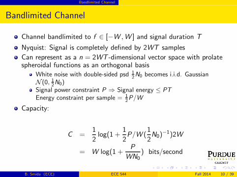
Bandlimited Channel
Channel bandlimited to f ∈ [−W ,W ] and signal duration T
Nyquist: Signal is completely defined by 2WT samples
Can represent as a n = 2WT -dimensional vector space with prolatespheroidal functions as an orthogonal basis
White noise with double-sided psd 12N0 becomes i.i.d. Gaussian
N (0, 12N0)
Signal power constraint P ⇒ Signal energy ≤ PTEnergy constraint per sample = 1
2P/W
Capacity:
C =1
2log(1 +
1
2P/W (
1
2N0)
−1)2W
= W log(1 +P
WN0) bits/second
B. Smida (ECE) ECE 544 Fall 2014 10 / 39
Bandlimited Channel
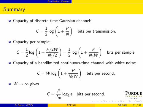
Summary
Capacity of discrete-time Gaussian channel:
C =1
2log
(1 +
P
N
)bits per transmission.
Capacity per sample:
C =1
2log
(1 +
P/2W
N0/2
)=
1
2log
(1 +
P
N0W
)bits per sample.
Capacity of a bandlimited continuous-time channel with white noise:
C = W log
(1 +
P
N0W
)bits per second.
W → ∞ gives
C =P
N0log2 e bits per second.
B. Smida (ECE) ECE 544 Fall 2014 11 / 39
Bandlimited Channel
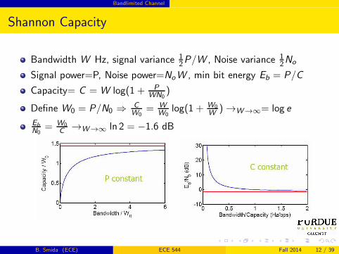
Shannon Capacity
Bandwidth W Hz, signal variance 12P/W , Noise variance 1
2No
Signal power=P, Noise power=NoW , min bit energy Eb = P/C
Capacity= C = W log(1 + P
WN0)
Define W0 = P/N0 ⇒ C
W0= W
W0log(1 + W0
W) →W→∞= log e
Eb
N0= W0
C→W→∞ ln 2 = −1.6 dB
B. Smida (ECE) ECE 544 Fall 2014 12 / 39
Bandlimited Channel
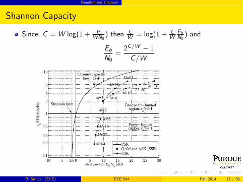
Shannon Capacity
Since, C = W log(1 + P
WN0) then C
W= log(1 + C
W
Eb
N0) and
Eb
N0=
2C/W − 1
C/W
B. Smida (ECE) ECE 544 Fall 2014 13 / 39

Practical Coding Schemes
Formal definition of Channel Coding
Definition: Channel code
An (M, n) code for the channel (X , p(y |x),Y) consists of the following:
1 An index set {1, 2, . . . ,M} over messages W .
2 An encoding function X n : {1, 2, . . . ,M} → X n, yielding codewordsxn(1), xn(2), . . . , xn(M). (This set is called the codebook C.)xn(W ) passes through the channel and is received as a randomsequence Y n ∼ p(yn | xn).
3 A (deterministic) decoding function
g : Yn → {1, 2, ., , , .M},
which is an estimator W = g(Y n) of W ∈ {1, 2, . . . ,M}. It declaresan error if W 6= W .
B. Smida (ECE) ECE 544 Fall 2014 14 / 39
Practical Coding Schemes
Practical Coding Schemes
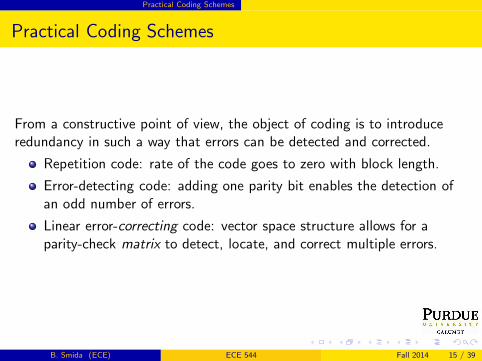
From a constructive point of view, the object of coding is to introduceredundancy in such a way that errors can be detected and corrected.
Repetition code: rate of the code goes to zero with block length.
Error-detecting code: adding one parity bit enables the detection ofan odd number of errors.
Linear error-correcting code: vector space structure allows for aparity-check matrix to detect, locate, and correct multiple errors.
B. Smida (ECE) ECE 544 Fall 2014 15 / 39
Practical Coding Schemes
Linear Block Codes
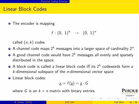
The encoder is mapping
f : {0, 1}k → {0, 1}n
called (n, k) codes
A channel code maps 2k messages into a larger space of cardinality 2n.
A good channel code would have 2k messages all evenly and sparselydistributed in the space.
A block code is called a linear block code iff its 2k codewords form ak-dimensional subspace of the n-dimensional vector space
Linear block codes:x = f (s) = s · G
where G is an k × n matrix with binary entries.
B. Smida (ECE) ECE 544 Fall 2014 16 / 39

Practical Coding Schemes
Properties of Linear Codes
The codebook of a linear code is
C ={x ∈ {0, 1}n : x = s · G for some s ∈ {0, 1}k
}
0n = G · 0k is always a codeword
if x1, x2 ∈ C , then x1 + x2 = (s1 + s2) · G is also a codeword
For any (n, k) linear code, there exists a parity check matrix H ofdimension (n − k)× n such that
x · HT = 01×(n−k) iff x ∈ C
This implies that G · HT = 0k×(n−k) .
B. Smida (ECE) ECE 544 Fall 2014 17 / 39

Practical Coding Schemes
Properties of Linear Codes
If C is a code with a generating matrix G in standard form,
G = [Ik |A],
where Ik denotes the identity matrix and A is some k × (n − k)matrix, then
H = [AT |In−k ]
is a check matrix for C.
dmin = minx∈C |x | is closely related to the error correcting ability ofthe code.
If a code has a minimum distance dmin, it is guaranteed to correct⌊(dmin − 1)/2⌋ errors.
B. Smida (ECE) ECE 544 Fall 2014 18 / 39

Practical Coding Schemes
Syndrome: Definition and properties
The generating matrix G is used in the encoder at the transmitter.On the other hand, the parity check matrix H is used in the decodingoperation at the receiver.
If we express the received vector r as the sum of of the original code xand a vector e (r = x + e) then,
r · HT = x · HT + e · HT = 01×(n−k) + s
The syndrome depends only on the error pattern, and not on thetransmitted codeword.
All error patterns that differ by a code word have the same syndrome.
B. Smida (ECE) ECE 544 Fall 2014 19 / 39

Practical Coding Schemes
Reed-Muller Codes
Reed-Muller codes are listed as RM(d , r), where d is the order of thecode, and r is parameter related to the length of code, n = 2r .
Reed-Muller codes can be defined very simply by in terms of Booleanfunction. To define codes of length n = 2r , we need r vectors(v1, v2, . . . vr ).
A generating matrix for a Reed-Muller code of length n and order dcan be constructed like this:
1, v1, v2, . . . , vr , v1v2, vr−1vr , . . . (up to degree d)
RM(d, r) codes are parity check codes of length n = 2r , rate Rc = k
n
and minimum distance 2r−d , where
k = 1 +
(r1
)+ . . .+
(rd
)
B. Smida (ECE) ECE 544 Fall 2014 20 / 39

Practical Coding Schemes
Reed-Muller Codes: Examples
RM(1, r) codes are parity check codes of length n = 2r , rateRc = r+1
nand minimum distance n
2 .RM(1,3) has the following generating matrix:
G =
1 1 1 1 1 1 1 10 0 0 0 1 1 1 10 0 1 1 0 0 1 10 1 0 1 0 1 0 1
RM(2,3) has the following generating matrix:
G =
1 1 1 1 1 1 1 10 0 0 0 1 1 1 10 0 1 1 0 0 1 10 1 0 1 0 1 0 10 0 0 0 0 0 1 10 0 0 0 0 1 0 10 0 0 1 0 0 0 1
B. Smida (ECE) ECE 544 Fall 2014 21 / 39

Practical Coding Schemes
Construction of new codes from old
Dual code: If C is an (n, k) linear code, it is dual or orthogonal codeC⊥ is the set of the vectors which are
C⊥ = {u|u.v = 0 for all v ∈ C}.
If C has generator matrix G and parity check matrix H, then C⊥ hasgenerator matrix H and parity check matrix G .
Product Codes: A simple method of combining two codes.
If we have two systematic linear block codes C1(n1, k1) and C2(n2, k2),the product of these codes is an (n1n2, k1k2) linear block code.The minimum distance of the product code is dmin = dmin1dmin2
Concatenated Codes: In concatenated coding two codes, one binaryand one non-binary are concatenated such that the codewords of thebinary code are treated a symbols of the the non-binary code.
B. Smida (ECE) ECE 544 Fall 2014 22 / 39
Practical Coding Schemes
A first definition for cyclic codes
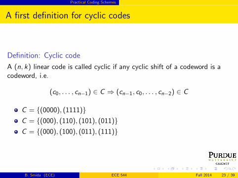
Definition: Cyclic code
A (n, k) linear code is called cyclic if any cyclic shift of a codeword is acodeword, i.e.
(c0, . . . , cn−1) ∈ C ⇒ (cn−1, c0, . . . , cn−2) ∈ C
C = {(0000), (1111)}C = {(000), (110), (101), (011)}C = {(000), (100), (011), (111)}
B. Smida (ECE) ECE 544 Fall 2014 23 / 39
Practical Coding Schemes
Cyclic codes: an algebraic correspondence
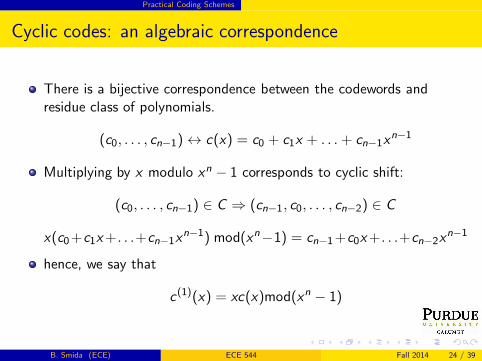
There is a bijective correspondence between the codewords andresidue class of polynomials.
(c0, . . . , cn−1) ↔ c(x) = c0 + c1x + . . .+ cn−1xn−1
Multiplying by x modulo xn − 1 corresponds to cyclic shift:
(c0, . . . , cn−1) ∈ C ⇒ (cn−1, c0, . . . , cn−2) ∈ C
x(c0+c1x+. . .+cn−1xn−1) mod(xn−1) = cn−1+c0x+. . .+cn−2x
n−1
hence, we say that
c(1)(x) = xc(x)mod(xn − 1)
B. Smida (ECE) ECE 544 Fall 2014 24 / 39
Practical Coding Schemes
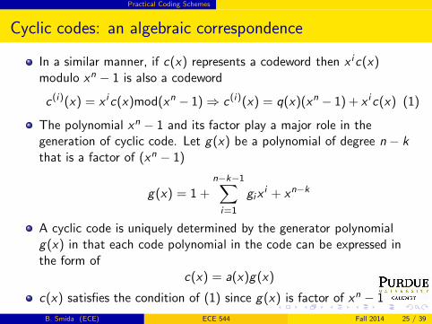
Cyclic codes: an algebraic correspondence
In a similar manner, if c(x) represents a codeword then x ic(x)modulo xn − 1 is also a codeword
c(i)(x) = x ic(x)mod(xn − 1) ⇒ c(i)(x) = q(x)(xn − 1) + x ic(x) (1)
The polynomial xn − 1 and its factor play a major role in thegeneration of cyclic code. Let g(x) be a polynomial of degree n− kthat is a factor of (xn − 1)
g(x) = 1 +
n−k−1∑
i=1
gixi + xn−k
A cyclic code is uniquely determined by the generator polynomialg(x) in that each code polynomial in the code can be expressed inthe form of
c(x) = a(x)g(x)
c(x) satisfies the condition of (1) since g(x) is factor of xn − 1
B. Smida (ECE) ECE 544 Fall 2014 25 / 39
Practical Coding Schemes
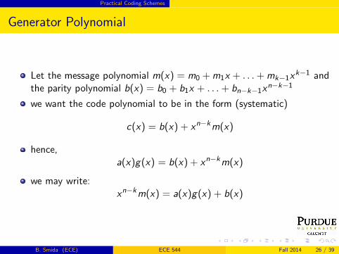
Generator Polynomial
Let the message polynomial m(x) = m0 +m1x + . . .+mk−1xk−1 and
the parity polynomial b(x) = b0 + b1x + . . .+ bn−k−1xn−k−1
we want the code polynomial to be in the form (systematic)
c(x) = b(x) + xn−km(x)
hence,a(x)g(x) = b(x) + xn−km(x)
we may write:xn−km(x) = a(x)g(x) + b(x)
B. Smida (ECE) ECE 544 Fall 2014 26 / 39

Practical Coding Schemes
Systematic Cyclic Encoder
1 Multiplying the message polynomial m(x) by xn−k
2 Dividing xn−km(x) by g(x) to obtain the remainder r(x)
3 Adding r(x) to xn−km(x)
B. Smida (ECE) ECE 544 Fall 2014 27 / 39
Practical Coding Schemes
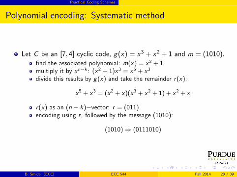
Polynomial encoding: Systematic method
Let C be an [7, 4] cyclic code, g(x) = x3 + x2 + 1 and m = (1010).
find the associated polynomial: m(x) = x2 + 1multiply it by xn−k : (x2 + 1)x3 = x5 + x3
divide this results by g(x) and take the remainder r(x):
x5 + x3 = (x2 + x)(x3 + x2 + 1) + x2 + x
r(x) as an (n − k)−vector: r = (011)encoding using r , followed by the message (1010):
(1010) ⇒ (0111010)
B. Smida (ECE) ECE 544 Fall 2014 28 / 39
Practical Coding Schemes
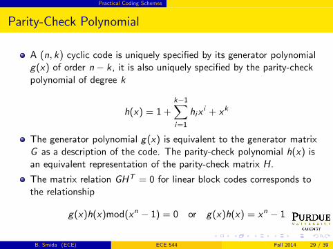
Parity-Check Polynomial
A (n, k) cyclic code is uniquely specified by its generator polynomialg(x) of order n− k , it is also uniquely specified by the parity-checkpolynomial of degree k
h(x) = 1 +
k−1∑
i=1
hixi + xk
The generator polynomial g(x) is equivalent to the generator matrixG as a description of the code. The parity-check polynomial h(x) isan equivalent representation of the parity-check matrix H.
The matrix relation GHT = 0 for linear block codes corresponds tothe relationship
g(x)h(x)mod(xn − 1) = 0 or g(x)h(x) = xn − 1
B. Smida (ECE) ECE 544 Fall 2014 29 / 39

Practical Coding Schemes
Generator and Parity-check Matrices
The generator polynomial g(x) is equivalent to the generator matrixG as a description of the code.
We may construct the generator matrix G by the k-polynomials:
g(x), xg(x), x2g(x), x3g(x), . . . , xk−1g(x)
The parity-check polynomial h(x) is an equivalent representation ofthe parity-check matrix H.
We define the reciprocal of the parity-check polynomial as:
xkh(x−1) = 1 +
k−1∑
i=1
hk−ixi + xk
which is also a factor of xn − 1
The following (n − k) polynomials may now be used in rows of the Hmatrix:
xkh(x−1), xk+1h(x−1), . . . , xn−1h(x−1)
B. Smida (ECE) ECE 544 Fall 2014 30 / 39

Practical Coding Schemes
Encoder for cyclic codes: feedback register
B. Smida (ECE) ECE 544 Fall 2014 31 / 39
Practical Coding Schemes
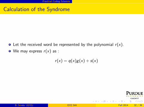
Calculation of the Syndrome
Let the received word be represented by the polynomial r(x).
We may express r(x) as :
r(x) = q(x)g(x) + s(x)
B. Smida (ECE) ECE 544 Fall 2014 32 / 39
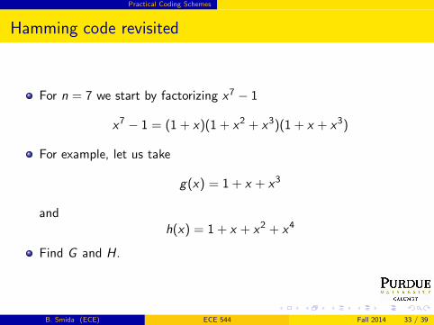
Practical Coding Schemes
Hamming code revisited
For n = 7 we start by factorizing x7 − 1
x7 − 1 = (1 + x)(1 + x2 + x3)(1 + x + x3)
For example, let us take
g(x) = 1 + x + x3
andh(x) = 1 + x + x2 + x4
Find G and H.
B. Smida (ECE) ECE 544 Fall 2014 33 / 39
Practical Coding Schemes
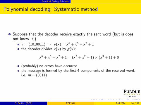
Polynomial decoding: Systematic method
Suppose that the decoder receive exactly the sent word (but is doesnot know it!)
v = (1010011) ⇒ v(x) = x6 + x5 + x2 + 1the decoder divides v(x) by g(x):
x6 + x5 + x2 + 1 = (x3 + x2 + 1)× (x3 + 1) + 0
(probably) no errors have occurredthe message is formed by the first 4 components of the received word,i.e. m = (0011)
B. Smida (ECE) ECE 544 Fall 2014 34 / 39
Practical Coding Schemes
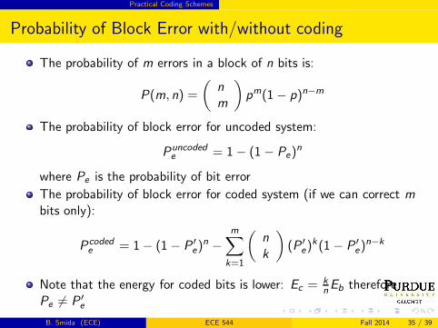
Probability of Block Error with/without coding
The probability of m errors in a block of n bits is:
P(m, n) =
(nm
)pm(1− p)n−m
The probability of block error for uncoded system:
Puncodede = 1− (1− Pe)
n
where Pe is the probability of bit error
The probability of block error for coded system (if we can correct mbits only):
Pcodede = 1− (1− P ′
e)n −
m∑
k=1
(nk
)(P ′
e)k(1− P ′
e)n−k
Note that the energy for coded bits is lower: Ec = k
nEb therefore
Pe 6= P ′e
B. Smida (ECE) ECE 544 Fall 2014 35 / 39
Joint source and channel coding
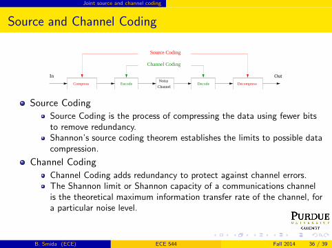
Source and Channel Coding
Out
Channel Coding
Source Coding
Compress Encode Decode DecompressNoisy
Channel
In
Source Coding
Source Coding is the process of compressing the data using fewer bitsto remove redundancy.Shannon’s source coding theorem establishes the limits to possible datacompression.
Channel Coding
Channel Coding adds redundancy to protect against channel errors.The Shannon limit or Shannon capacity of a communications channelis the theoretical maximum information transfer rate of the channel, fora particular noise level.
B. Smida (ECE) ECE 544 Fall 2014 36 / 39
Joint source and channel coding
Source-Channel Separation Theorem
So far we have R > H (compression) and R < C (transmission). It isnatural to ask whether the condition H < C is necessary and sufficient fortransmitting a source over a channel:
Theorem: Source-channel coding theorem
If V1,V2, . . . ,Vn is a finite-alphabet stochastic process satisfying the AEPand the condition H(V) < C , then there exists a source-channel code withprobability of error Pr(V n 6= V n) → 0.Conversely, if for any stationary stochastic process we have thatH(V) > C , then the probability of error is bounded away from zero.
Important result: source coding and channel coding might as well bedone separately since same capacity
B. Smida (ECE) ECE 544 Fall 2014 37 / 39