9/10/2015

1

Changing Mindsets:

A Passive-First Artificial Sky

Bruce Haglund, Emilie Edde, Daniel Flesher, and Brenda Gomez

University of Idaho, Moscow, Idaho

…from napkin sketch to realization?

Redesign:

Experimenting with translucent

ceiling and neutral floor materials.

And, ultimately with different shapes.

9/10/2015

2

Two teams proposed Mirror-Box Sky w/Kalwall Skylight.

First Feasible Option:

Daylighted vs. Electrically Lighted

Second Feasible Option:

Two teams proposed Conical Sky w/matte white interior.

Culplight analysis image

9/10/2015

3

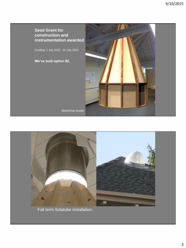
Seed Grant for

construction and

instrumentation awarded

Funding: 1 July 2012 - 31 July 2014.

We’ve built option #2.

SketchUp model

Fall term Solatube installation

9/10/2015

4

Spring term construction sequence

Using Photography for Testing and Calibration:

Pros.1. Photography can collect luminance data for all points simultaneously

2. Photography can act as a per pixel luminance meter when calibrated properly, resulting in extremely high-resolution measurements

9/10/2015

5

Using Photography for Testing and Calibration:

Cons.1. All lenses exhibit vignetting, or the darkening of pixels at the corners of

the photos. This phenomena must be accurately corrected for in order to be used for analysis.

2. Vignetting affected not only by lens, but by aperture size, so all photos must be taken at same aperture for correction to remain constant.

http://upload.wikimedia.org/wikipedia/commons/1/1f/Example_of_vignetting_and_dusty_scan.jpg

Calibration Process:

Area of interest defined within

white partition. Light level

measured 26.4fL at top and

20.3fL at bottom

Relatively even distribution.

Value will be averaged in

5°increments to determine

light falloff, expressed as a

quartic function.

9/10/2015

6

Calibration Process:

Camera placed on a tripod and rotated 5° between exposures.

F-4 with 1/6s exposure.

Calibration Process:

Area of interest cropped in Photoshop, resulting in a continuous image

of the same spot from 0-90°

0°5°10°15°20°25°30°35°40°45°50°55°60°65°70°75°80°85°90°

9/10/2015

7

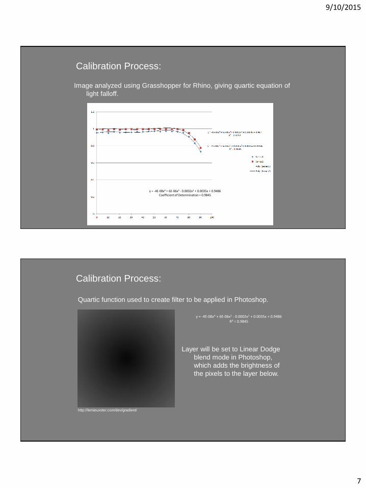
Calibration Process:

Image analyzed using Grasshopper for Rhino, giving quartic equation of

light falloff.

y = -4E-08x4 + 6E-06x3 - 0.0002x2 + 0.0035x + 0.9486Coefficient of Determination = 0.9845

Calibration Process:

Quartic function used to create filter to be applied in Photoshop.

http://lemieuxster.com/dev/gradient/

y = -4E-08x4 + 6E-06x3 - 0.0002x2 + 0.0035x + 0.9486R² = 0.9845

Layer will be set to Linear Dodge

blend mode in Photoshop,

which adds the brightness of

the pixels to the layer below.

9/10/2015

8

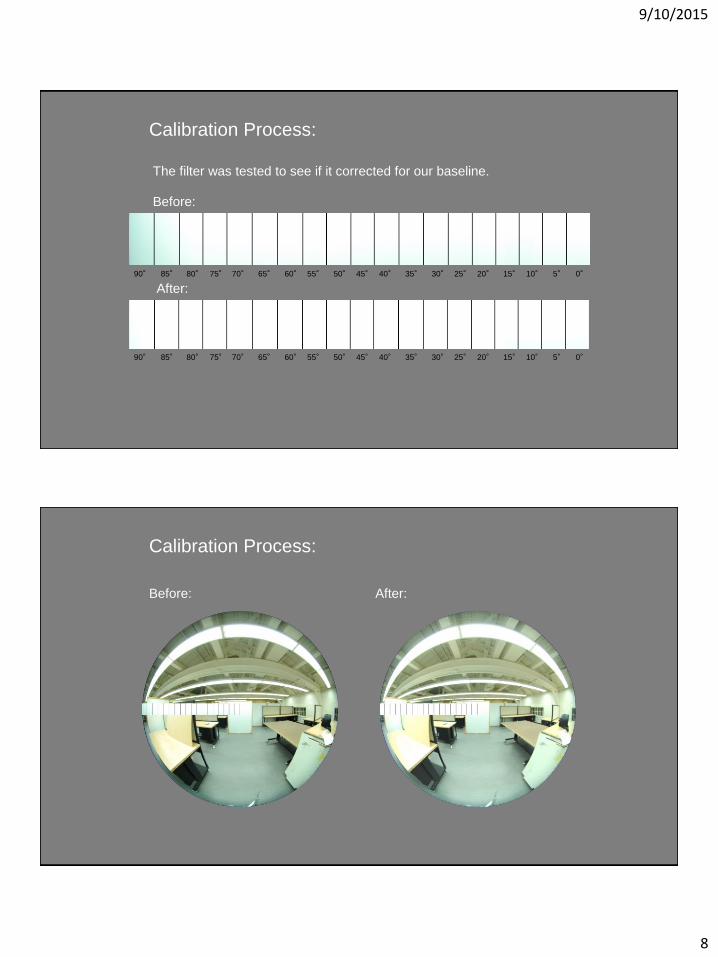
Calibration Process:

The filter was tested to see if it corrected for our baseline.

Before:

After:

0°5°10°15°20°25°30°35°40°45°50°55°60°65°70°75°80°85°90°

0°5°10°15°20°25°30°35°40°45°50°55°60°65°70°75°80°85°90°

Before:

Calibration Process:

After:

9/10/2015

9

Calibration Process:

The image with applied filter was analyzed in Grasshopper to see if light

fall off had actually been corrected.

Testing the Sky Using Photography

Photo taken using fisheye lens inside artificial sky on Oct 14th 2013 at

2:20PM; Clear sky conditions.

Lens pointed directly at zenith and positioned at the height of the

horizon.

Photo corrected for vignetting.

Before: After:

9/10/2015

10

Testing the Sky Using Photography

Corrected photo analyzed using Grasshopper plug-in for Rhino

Testing the Sky Using Photography

Graphed measurements in Excel

North South

9/10/2015

11

Next Steps

Sky needs to be tested for morning, noon, and evening light levels

during overcast, clear, and partly cloudy sky conditions, and during

all seasons.

Sky needs some adjustment since the horizon is 50% as bright as zenith

instead of target 33%.

DATA ACQUISITION SCHEMES

Data Acquisition System

Software:

Personal DAQView Plus

Hardware:

OMB-DAQ-55; Li-Cor Photo Sensors; Millivolt adapters; Host PC

Calibration:

5 Li-Cor photo sensors were tested individually in the same spot under the same artificial lighting conditions and multiplied by their specific calibration per millivolt

Fisheye Lens

Components: Fisheye Lens; Fisheye Projections on Dot Diagram

9/10/2015

12

Millivolt Adapter

Photo Sensor

Data Acquisition System

Analog In/Out

Host PC

Connection

DAQ Set-Up/Testing:

9/10/2015

13

Sky Envelope

Outside Inside

Scale Model

DAQ Testing: (Plan View)

1A mV 1B mV 1C mV

2A mV 2B mV 2C mV

3A mV 3B mV 3C mV

4A mV 4B mV 4C mV

5 mV

(Top of Model)

1 Outside of

Scale Model

(Unobstructed)

4 Sensors Inside

of Scale Model

DF calculated

per square

(12)

DAQ Software: Personal DAQView Plus

Variable

9/10/2015

14

Scale Model

DAQ Testing/Results: (Plan View)

1A klux 1B klux 1C klux

2A klux 2B klux 2C klux

3A klux 3B klux 3C klux

4A klux 4B klux 4C klux

5 klux

DF calculated per square (12)

Calculations:

Multiply the Calibration Factor

(specific to each sensor) in klux per

mV = Ei per square

DF= Ei/Eo x 100%

DAQ Data Input

Sensor Location Physical Channel Photo Sensor Scale Analog Input Reading Calibration Factor Reading in klux Daylight Factor DF Results

SN Number (995-) mV mV (millivolt)2290 Multiplier (klux/mV) After Multiplier Decimal %

Inside Model PD1_A01 (1L/H) PH9954 5159.33 -0.013 -5.16 0.06708 0.01364574 1.36457397

Inside Model PD1_A02 (2L/H) PH9955 4976.34 -0.016 -4.98 0.07968 0.016208893 1.62088929

Inside Model PD1_A03 (3L/H) PH9956 5844.08 -0.021 -5.84 0.12264 0.024948025 2.49480249

Inside Model PD1_A04 (4L/H) PH9957 5260.98 -0.018 -5.26 0.09468 0.019260266 1.92602658

Outside Model PD1_A05 (5L/H) PH9958 5113.12 -0.962 -5.11 4.91582 n/a n/a

VariableDaylight Factor

per square

9/10/2015

15

Scale Model

DAQ Results: (Plan View)

1A% 1B% 1C%

2A% 2B% 2C%

3A% 3B% 3C%

4A% 4B% 4C%

5%

DF= Ei/Eo x 100%

Scaled Model: UI Swim Center

(One large open space with roof

monitors)

Fisheye Lens:

9/10/2015

16

Fisheye Lens: Dot Projection Method

0* 30*

60* 90*

Horizontal Sky Component

Equal Solid Angle Projection

Each dot represents 0.1%

# of Dots

0*= 32

30*= 19

60*= 24

90*= 24

Ave:

21.25

Or 2.125%

Fisheye Lens: Dot Projection Method

• Steps Following the Sky Component:

- Externally reflected component

- # of dots on external surfaces / by 5

- 1/5 of sky obstruction

- Internally reflected component

- Calc. avg. DF using BRE formula or Vertical Daylight Factor x (avg. room reflectance)2

- Add all components

- D = sky component + external + internal

- rounded to nearest whole # or nearest 0.5%

9/10/2015

17

Next Test: Lighting Seminar

Designs for 1912 Center

Physical model for use in artificial sky

Filip Fichtel, Ryan McColly, Clay Reiland

9/10/2015

18

Comparing physical model in sky with outdoors:

Tom Kearns, Ryan Ivie, Ben Ferry, Clay Cravea

Ou

tdo

ors

In

Sky

0

50

100

150

200

250

300

-90

-85

-80

-75

-70

-65

-60

-55

-50

-45

-40

-35

-30

-25

-20

-15

-10 -5 0 5 10 15 20 25 30 35 40 45 50 55 60 65 70 75 80 85 90

Chart Title

X y z z2

0

50

100

150

200

250

300

Chart Title

x y z z2

BEFORE

AFTER

Before and after installation of temporary baffle.

9/10/2015

19

More work to do:

1. Analyze photos from different seasons and sky conditions

2. Adjust sky aperture (the baffle) as needed

3. Retest and reanalyze

4. Write Users’ Manual

5. Distribute plans worldwide