changes in subjective versus objective well-being in india
TRANSCRIPT

University of Pennsylvania University of Pennsylvania
ScholarlyCommons ScholarlyCommons
Population Center Working Papers (PSC/PARC) Penn Population Studies Centers
5-12-2021
Changes in Subjective versus Objective Well-Being in India Changes in Subjective versus Objective Well-Being in India
Vani S. Kulkarni University of Pennsylvania, [email protected]
Veena S. Kulkarni Arkansas State University - Main Campus, [email protected]
Katsushi S. Imai University of Manchester, [email protected]
Raghav Gaiha University of Pennsylvania, GDI University of Manchester, [email protected]
Follow this and additional works at: https://repository.upenn.edu/psc_publications
Part of the Demography, Population, and Ecology Commons, Diseases Commons, Education
Commons, Family, Life Course, and Society Commons, and the Inequality and Stratification Commons
Recommended Citation Recommended Citation Kulkarni, Vani, Veena Kulkarni, Katsushi Imai, and Raghav Gaiha. 2021. "Changes in Subjective versus Objective Well-Being in India." University of Pennsylvania Population Center Working Paper (PSC/PARC), 2021-71. https://repository.upenn.edu/psc_publications/71.
This paper is posted at ScholarlyCommons. https://repository.upenn.edu/psc_publications/71 For more information, please contact [email protected].
Changes in Subjective versus Objective Well-Being in India Changes in Subjective versus Objective Well-Being in India
Abstract Abstract Although there is abundant literature on subjective well-being (SWB), there is virtually none for India. Growing recognition of the validity and accuracy of measures of SWB of well-being underlies the rapid growth of literature on SWB in recent decades but it has mainly focused on developed countries. Ours is, to our knowledge, the first study of SWB at the all-India level, and one of the few on developing countries, with a rigorous validation of the results. Applying robust OLS and ordered probit models to the India Human Development Survey (IHDS) panel data in 2005 and 2012, we assess SWB changes in 2005-2012, based on a self-reported measure of changes in economic well-being, as a function of household and state covariates in 2005. This is in sharp contrast with earlier studies’ focus on the levels of SWB. Another point of departure of our study and an innovative extension is to compare the covariates of SWB changes with those of objective well-being (OWB) changes, proxied by the relative growth in real per capita household consumption between 2005 and 2012. Households with an older and educated head in a larger household, located in urban areas or affluent states in 2005 tend to experience further improvement in both SWB and OWB between 2005 and 2012. On the contrary, households with a female household head, with more male members in the labour market, with regular access to mass media, without members suffering from non-communicable diseases or disability are more likely to be better off subjectively without experiencing corresponding improvement in OWB. The policy challenges raise serious concerns.
Keywords Keywords subjective well-being, affluence, age, health, caste, religion, India
Disciplines Disciplines Demography, Population, and Ecology | Diseases | Education | Family, Life Course, and Society | Inequality and Stratification | Social and Behavioral Sciences | Sociology
This working paper is available at ScholarlyCommons: https://repository.upenn.edu/psc_publications/71

1
Edited 12 May 2021
Changes in Subjective versus Objective Well-Being in India1
Vani S. Kulkarni,University of Pennsylvania, [email protected],
Veena S. Kulkarni, Arkansas State University - Main Campus, [email protected],
Katsushi S. Imai, University of Manchester, [email protected]
Raghav Gaiha2, University of Pennsylvania and GDI University of Manchester,
Abstract
Although there is abundant literature on subjective well-being (SWB), there is virtually
none for India. Growing recognition of the validity and accuracy of measures of SWB of
well-being underlies the rapid growth of literature on SWB in recent decades but it has
mainly focused on developed countries. Ours is, to our knowledge, the first study of
SWB at the all-India level, and one of the few on developing countries, with a rigorous
validation of the results. Applying robust OLS and ordered probit models to the India
Human Development Survey (IHDS) panel data in 2005 and 2012, we assess SWB
changes in 2005-2012, based on a self-reported measure of changes in economic well-
being, as a function of household and state covariates in 2005. This is in sharp contrast
with earlier studies’ focus on the levels of SWB. Another point of departure of our study
and an innovative extension is to compare the covariates of SWB changes with those of
objective well-being (OWB) changes, proxied by the relative growth in real per capita
household consumption between 2005 and 2012. Households with an older and educated
head in a larger household, located in urban areas or affluent states in 2005 tend to
experience further improvement in both SWB and OWB between 2005 and 2012. On the
contrary, households with a female household head, with more male members in the
labour market, with regular access to mass media, without members suffering from non-
communicable diseases or disability are more likely to be better off subjectively without
experiencing corresponding improvement in OWB. The policy challenges raise serious
concerns.
Key Words: Subjective Well-Being, Affluence, Age, Health, Caste, Religion, India.
JEL Codes: I31, I14, I38, J71, P35.
1We are indebted to Raj Bhatia for his invaluable contribution to the econometric analysis, and to A. J.
Oswald, Anil S. Deolalikar, S. Shankar, A. S. Venkatraman, N. Chandramohan and Radhika Aggarwal for
constructive suggestions. Above all, we are grateful to Jere Behrman for his guidance and valuable
suggestions. We appreciate valuable advice on the interpretations of IHDS by Sonalde Desai who led
IHDS. The views are personal and not necessarily of the institutions to which we are affiliated. 2 Corresponding Author: Raghav Gaiha, Email: [email protected]

2
Changes in Subjective versus Objective Well-Being in India
1. Introduction
Well-being is hard to define, and harder to measure. This, however, has not deterred
economists and other social scientists as well as pollsters from assessing it. Relying on
subjective measures of well-being, leading scholars have made important contributions to its
measurement and elaboration of its policy importance.
Following Steptoe et al. (2015), three aspects of subjective well-being can be distinguished -
evaluative well-being (or life satisfaction), hedonic well-being (feelings of happiness,
sadness, anger, stress, and pain), and eudemonic well-being (sense of purpose and meaning in
life).
Life evaluation refers to the quality or goodness of lives, overall life satisfaction, or
sometimes happiness. Measurement is usually based on the Cantril ladder (1965), wherein
individuals are asked to place themselves on an 11-step ladder with the worst possible life
representing the lowest rung and the best possible life representing the top rung. Hedonic
well-being refers to everyday feelings or moods such as experienced happiness (the mood,
not the evaluation of life), sadness, anger, and stress, and is measured by asking respondents
to rate their experience of several affect adjectives such as happy, sad, and angry. Eudemonic
well-being focuses on judgments about the meaning and purpose of one’s life; because the
concept is more diverse, several questionnaires exploring various aspects of meaning have
been developed (Steptoe et al. 2015).
Measures of SWB (life evaluation or overall life satisfaction) have been controversial.
Ravallion et al. (2016), for example, are sceptical but not dismissive of such measures. Their
scepticism rests on scale heterogeneity-the standard deviation of utility over different choice
situations. However, subjective measures of poverty are not just similar to those obtained
from income/expenditure thresholds but sometimes unavoidable3. Deaton (2018), however,
offers robust support to self-reported measures of well-being, as such measures capture
aspects of welfare beyond real income, which is what economists typically use to proxy
utility. He uses cross-country and country-specific comparisons to validate measures of
SWB, and draws out their policy significance.
Strands of the literature show that the relationship between well-being and age is U-shaped -
well-being is at its lowest among the middle-aged (35-45 years), and highest in the oldest 75-
plus age group. This is justified in terms of work-related stress and uncertainty about the
future, while at much older ages, there is freedom from work-related stress and, perhaps, a
3In another important contribution, Ravallion (2014) conjectures that different people are likely to have
different ideas about what it means to be “rich” or “poor,” or “satisfied” or not with one’s life, leading
them to interpret survey questions on subjective welfare differently.

3
sense of accomplishment (Blanchflower and Oswald, 2007, Dolan et al. 2008, among others).
Deaton (2018), however, offers a more balanced appraisal. Age patterns are neither universal,
nor very pronounced. Specifically, the (unconditional) U-shape appears in the English
speaking countries, to a lesser extent in East and in South Asia, and in (non-English
speaking) Europe - more for men than women - but not elsewhere. Even in the US, using the
nationally representative survey data (General Social Survey) in 1973-1994, Easterlin (2006)
showed that the relationship between age and happiness represents an inverted U-shape curve
where the happiness measure is on family and health satisfaction. That is, the happiness of a
birth cohort rises mildly from age 18 to midlife, and declines after 50. So the age-wellbeing
relationship cannot be generalised as it differs considerably depending on the study context
(e.g. differences of country or regions, time, the definition of well-being, the nature of the
data).
Our objective is to identify and assess the factors associated with changes in SWB in India
between 2004-5 and 2011-12. We carry out econometric analyses using the large panel
dataset constructed by India Human Development Surveys (IHDS) 1 and 2. These surveys
form a national panel household survey covering all parts of India and were organised by the
University of Maryland and the National Council of Applied Economic Research.4It must be
pointed out, however, that the measure of SWB that we use is focused on perceived economic
well-being of the household, such as a respondent (or a household head) perceived that the
household is economically better-off (2), just the same (1) and worse-off (0) between 2004-5
and 2011-12. To mitigate the endogeneity concern, we estimate this discrete dependent
variable by a number of explanatory variables at household, community and state levels in
2004-5 (e.g. demographic and other variables such as age, health, caste, religion, location,
and conflicts) using robust Ordinary Least Squares (OLS) and ordered probit models5.
Another objective is to compare factors associated with SWB changes with those of objective
well-being (OWB). The latter is proxied by the relative growth in real per capita household
consumption in 2004-5-2011-2. We have classified the entire sample into three groups,
better-off (2), just the same (1) and worse off (0) based on the ranking of the real per capita
household consumption growth, making the frequency distributions across the three
categories identical to those of SWB changes to make the coefficient estimates comparable in
their sign and size. We aim to assess the factors associated with SWB changes, not with
OWB changes, to identify the specific covariates of SWB changes. To our knowledge, this is
one of the few studies to compare SWB and OWB or their changes in terms of their
covariates.6While aiming to contribute to the aforementioned academic literature on SWB,
we will pay particular attention to policy concerns arising from our results.
The rest of the study is organised as follows. Section 2 gives a selective review of important
contributions to the rapidly growing literature on SWB. Section 3 discusses salient features of
4https://ihds.umd.edu/data (accessed on 22 February 2021). 5 Although this does not overcome the endogeneity of some of the explanatory variables, it allows us to rule out
reverse causality.. 6 A notable exception is Oswald and Wu (2010) who found a close correlation between SWB and OWB
measures at the state level in the U.S.A.

4
the data, while showing the associations between the SWB change (or the OWB change) and
key covariates, based on cross-tabulations. Section 4 offers brief expositions of multiple
regression and ordered probit (OP) models for SWB and OWB changes. Section 5 is devoted
to interpretation of the results obtained by multiple regression and OP. Section 6 concludes
by discussing the significance of our results and the policy challenges.
2. Literature Review
One important empirical issue is whether the measures of subjective well-being (SWB) are
reliable (e.g., Kahneman and Krueger, 2006; Kahneman and Deaton, 2010; Diener et al.,
2013; Akay et al., 2017, and Deaton, 2011, 2018).
Kahneman and Krueger (2006) review the literature on SWB, including their own studies,
and argue that the income level is not necessarily associated with better SWB and that one
way of partially assessing the validity of SWB measures is to examine their correlation with
various individual traits. Drawing upon empirical studies of SWB, the authors argue that (i)
recent positive changes in circumstances, as well as demographic variables including
schooling and health, are likely to be positively correlated with happiness or satisfaction;(ii)
variables that are associated with low life satisfaction and happiness include: recent negative
changes of circumstances; chronic pain; and unemployment, especially if only the individual
concerned was laid off; (iii)gender is uncorrelated with life satisfaction and happiness; (iv)
the effects of age are complex—the lowest life satisfaction is apparently experienced by those
who have teenagers at home, and reported satisfaction improves thereafter. They resolve the
puzzle of the relatively small and short-lived effect of changes in most life circumstances on
reported life satisfaction by invoking evidence on adaptability. They conclude that despite
their limitations, subjective measures of well-being enable welfare analysis in a more direct
way that could be a preferred alternative to traditional welfare analysis.
Another important study by Diener et al. (2013) scrutinises the life satisfaction scales in the
global context based on their critical review of relevant studies and verifies the reliability of
the scales used and validity of judgments made in SWB measures. The stability of life
satisfaction scores across time and situations suggests that consistent psychological processes
are involved and similar information is used when people report their scores, while single-
item scales are less stable than multi-item life satisfaction scales. Societal-level mean life
satisfaction also shows robust consistency. In the Gallup World Poll, for example, in which
there was an identical life evaluation question in the identical item-order collected over years,
there is a .93 correlation across waves of the data for 1-year intervals (N = 336 nation-wave
pairs), and a .91 correlation across a 4-year interval (N = 74 nations).To summarise the
authors’ findings, reliability and validly of life satisfaction scales reflect authentic differences
in the ways people evaluate their lives, and the scores move in expected ways to changes in
people’s circumstances.
Among those who have emphatically endorsed SWB measures is Deaton (2018). He argues
that SWB measures do not need to be related to behaviour. ‘If decision utility differs from
welfare utility, and if people sometimes behave against their best interests, the direct

5
measurement of well-being might still give an accurate measure, and might even enable
people to do better, either through paternalistic government policies, or incentives, but more
simply by providing information on the circumstances and choices that promote well-
being…’(ibid., 2018, p. 18). Deaton elaborates that direct measures may also capture aspects
of welfare beyond real income, which is what economists typically use to proxy utility.
Health is a case in point; education, civil liberties, civic participation, respect, dignity, and
freedom are others. Our study focusing on SWB and OWB changes is in line with Deaton’s.
Deaton (2018), based on the Gallup World Poll, uses an evaluative measure of well-being
that asks people to report, on an eleven-point scale, from 0 to 10, how their life is going. The
question is originally due to Cantril (1965), and is asked in exactly the same way of all
individuals sampled by Gallup in their World Poll. The question is “Please imagine a ladder,
with steps numbered from 0 at the bottom to 10 at the top. The top of the ladder represents
the best possible life for you and the bottom of the ladder represents the worst possible life
for you. On which step of the ladder would you say you personally stand at this
time?”(Deaton, 2018, p. 19).
His main findings are: average ladder values vary greatly around the world, from around 4 in
Africa, to between 7 and 8 for the rich countries of Europe and the English-speaking world;
differences between men and women within regions are smaller than differences between
regions; women tend to evaluate their lives somewhat more highly than men, except in
Africa, and sometimes among those over 60; age patterns are apparent, but neither universal,
nor very pronounced, at least compared with those associated with international differences
in incomes; the (unconditional) U-shape appears in the English speaking countries (U.K.,
U.S., Canada, Ireland, New Zealand and Australia), to a lesser extent in East and in South
Asia and perhaps in Latin America and the Caribbean - though only in the last age group (65-
74), and in Europe—more for men than women—but not elsewhere. In the two poorest
regions, Africa and South Asia, life evaluation is low throughout life and, in Africa, it falls
with age. However, he is puzzled by the U-shape of well-being, where it exists, since SWB
rises after middle-age, when people are losing their spouses, and when both morbidity and
mortality are rising. In contrast, other components of psychological well-being may improve
with age, less stress, and the negative side-effects (e.g., physical pain) of work diminish with
retirement.
In a highly cited study, Blanchflower and Oswald (2007) analyse data on 500,000 Americans
and Europeans. It draws two main conclusions. First, psychological well-being depends in a
curvilinear way upon age. Second, there are important differences in the reported happiness
levels of different birth-cohorts. The results draw upon regressions and use datasets covering
the period long enough to distinguish age effects from cohort effects. The authors suggest
that reported well-being is U-shaped in age and that the convex structure of the curve is
similar across different parts of the Western world. A limitation is that the analysis does not
track the same individuals over time.
In an admirably clear and comprehensive review of factors associated with SWB, Dolan et al.
(2008) draw attention to ambiguities, inconsistencies and causality in the interpretation of the

6
results. The results generally show positive but diminishing returns to income. Some of this
positive association is likely to be due to reverse causation, as indicated by the studies which
show higher well-being leading to higher future incomes (Clark, Frijters, and Shields, 2008).
Studies that have included relative income (defined in a range of different ways with a range
of different reference groups) suggest well-being is strongly affected by relativities. So, if
additional income rises by similar amount in a person’s reference group, it is unlikely to be
associated with gains in SWB (Dorn et al. 2007)7.Indeed, much evidence indicates that rank
in the income distribution influences life satisfaction. However, no studies have so far
compared the covariates of SWB and those of the ranks defined by economic measures, that
is, OWB.
Earlier studies consistently find a negative relationship between SWB and age and a positive
relationship between age squared and SWB, which is consistent with a U-shaped curve in the
SWB-age domain. For example, Blanchflower and Oswald (2007) show that well-being tends
to be higher at the younger and the older age points, and lower at the middle age point8.
Women tend to report higher happiness but worst scores on the GHQ (Alesina, et al., 2004),
although a few studies report no gender differences even using the same datasets. This is not
surprising as specifications differ (Dolan et al. 2008).
Some studies find a positive relationship between SWB and each additional level of
schooling, while others find that middle level of schooling is related to the highest life
satisfaction (e.g., Blanchflower & Oswald, 2004, Stutzer, 2004). However, there is some
evidence that schooling has more of a positive impact in low income countries. In addition,
the coefficient on schooling is often responsive to the inclusion of other variables within the
model. Schooling is likely to be positively correlated with income and health, and, if these are
not controlled for, the schooling coefficient is likely to be more strongly positive (Fahey &
Smyth, 2004; Ferrer-i-Carbonell, 2005).
Evidence shows a large negative effect of individual unemployment on SWB. Models, which
treat life satisfaction scales as a continuous variable, tend to find that the unemployed have
around 5-15% lower scores than the employed. Men have been found to suffer most from
unemployment and some studies also find that the middle- aged suffer more than the young
or old (e.g., Di Tella et al., 2001, Clark, 2003).While the evidence is relatively clear that
employment is better than unemployment, the relationship between the amount of work (e.g.,
number of hours worked) and well-being is less straightforward. An interesting result is an
inverted U-shaped curve between life satisfaction and hours worked suggesting that well-
being rises as hours worked rise but only up to a certain point and then starts to drop as hours
become longer (Meir and Stutzer, 2006).
7Much of the credit is due to Duesenberry (1949) who argued that relative income rather than the level of
income affects well-being – earning more or less than others looms larger than how much one earns. 8As noted earlier, this view is not corroborated in more recent studies of Africa and South Asia (Deaton,
2018).

7
Studies consistently show a strong relationship between SWB and both physical and
psychological health. Psychological health appears to be more highly correlated with SWB
than physical health but this is not surprising given the close correspondence between
psychological health and SWB. Some of the association may be caused by the impact that
well-being has on health but the effect sizes of the health variables are substantial, suggesting
that, even after accounting for the impact of SWB on health, the effect of health on SWB is
still significant (Kohler et al. 2017). Furthermore, specific conditions, such as heart attacks
and strokes reduce well-being, and the causality here is more likely to be from the health
condition to SWB. Hence, deliberate exclusion of health variables, as suggested by
Blanchflower and Oswald (2007), is problematic. Specifically, the omitted variable bias is
likely to be large and thus our study controls for both non-communicable diseases (NCDs)
and disabilities of household members.
The evidence is fairly consistent and suggests that regular engagement in religious activities
is positively related to SWB. While some studies only examine whether or not the person
actually attends church, others examine different amounts of time spent in these activities.
Using World Values Survey (WVS) data, Helliwell (2003) finds higher life satisfaction to be
associated with church attendance of once or more a week. On the related issue of religiosity
(e.g., regular attendance of church), Deaton (2011) offers valuable insights. At least on
average, over all countries, and over countries disaggregated into income groups, religious
people do better on a number of health and health-related indicators. These protective effects
appear to be stronger the poorer is the country, as religion is a route to a better life in poor
countries, but not in rich ones, and stronger for men than women.
Generally, being alone appears to be worse for SWB than being part of a partnership.
Although there is some variation across studies, it seems that being married is associated with
the highest level of SWB and being separated is associated with the lowest level of SWB,
lower even than being divorced or widowed (e.g., Helliwell, 2003).
The evidence on the impact of income inequality on well-being is mixed. Based on the WVS
data, Fahey and Smyth (2004) find that inequality reduces life satisfaction, whereas Haller
and Hadler (2006) find that inequality increases life satisfaction. One conjecture for these
contrasting findings using international data may be that the inclusion of particular countries
influences the results. The evidence suggests that living in an unsafe or deprived area is
detrimental to life satisfaction, controlling for own income (Ferrer-i-Carbonell&Gowdy,
2007).Living in large cities is detrimental to life-satisfaction while living in rural areas is
beneficial, after controlling for income (e.g., Graham and Felton, 2006).
In India’s context, an important question is: Do Dalits and Other Backward Classes (OBC) in
rural North India report lower life satisfaction than higher caste people, and if so, is it merely
because they are poorer? Spears (2016) addresses this question, using the Sanitation Quality,
Use, Access and Trends (SQUAT) survey data collected in rural Bihar, Haryana, Madhya
Pradesh, Rajasthan and Uttar Pradesh in 2013–14 by a team of researchers, including the
author. Two specific issues are: (i) Do Dalits and Other Backward Classes (OBC) in rural
north India report lower life satisfaction than higher caste people, and, if so, (ii) is it merely

8
because they are poorer? The findings are: lower caste people in rural North India evaluate
their lives to be worse than higher caste people, and this difference is not explained by
income poverty. Spears (2016) is only among a few studies on SWB in the context of India
and, to our knowledge, there have not been any national-level studies on SWB in India. We
aim to fill the gap by using the nationally representative household survey data.
3. Data
Our analysis draws upon the two rounds of the nationally representative India Human
Development Survey (IHDS) data for 2004-5 and 2011-12, conducted jointly by the
University of Maryland and the National Council of Applied Economic Research, New Delhi.
The first round (IHDS-1) is a survey of 41,554 households in 2004-5. The second round
(IHDS-II) involves re-interviews with 83% of the original households as well as split
households residing within the same locality, along with an additional sample of 2,134
households in 2011-129. The total for IHDS-II is therefore 42,152 households. The sample is
spread across 33 (now 34) states and union territories, and covers rural as well as urban areas.
Repeated interviewing of the same households at two points in time facilitates a richer
understanding of which households are able to partake in the fruits of growth, what allows
them to move forward, and the process through which they are incorporated into or left out of
a growing economy.
Topics covered by the IHDS relevant in the present context include the perceived changes in
subjective well-being (SWB), expenditure, income, employment, major morbidity (including
non-communicable diseases (NCDs)), limitations in activities of daily living (ADLs), health
insurance, castes, religion, assets, social networks (e.g., self-help groups), trust in institutions,
conflicts, crimes, exposure to mass media, and demographic characteristics (e.g. gender, age,
marital status, household size and composition)10.
An important feature of IHDS is that it collected data on SWB changes. The question asked
is: “Compared to 7 years ago, would you say your household is economically doing the same,
better or worse today?” So the focus of this SWB is narrow and it has only three scales
corresponding to the perceived change in the SWB (denoted as ∆SWB hereafter), not its
level. It should also be noted that the measure is at the household level, not the individual
level. While the focus of this variable is narrow, it has a few advantages. First, as reviewed in
9An additional sample of 2134 households was added to the urban sample of IHDS-II to reduce the impact
of attrition on the standard errors of a few key variables. The simulations estimated that the attrition would
increase standard errors to unacceptable levels if 8 out of 15 households were unreachable in each urban
cluster. Hence, the interviewers were asked to report to NCAER supervisors if they were unable to
recontact 5 or more households in a cluster. The supervisor verified the losses and randomly assigned
households to the right, the left, or at the original location based on the original locations of the households
which were not observed in 2011-12 using a predefined rule. A similar addition to the rural sample was not
attempted because of much lower attrition rates (Personal communication with a scholar who led IHDS). 10It is noted that the IHDS-1 in 2005 does not allow identification of the respondent, while the IHDS-2 in
2012 does. As the respondents reported SWB changes in 2005-12 at the household level in IHDS-2, we
have matched SWB or OWB changes, a dependent variable, to household head’s characteristics, and other
explanatory variables, by restricting the sample only to the cases where the household head data are
available.

9
detail in the previous section, there exists a life-cycle effect on SWB, that is, perceived well-
being changes at the point of life-cycle or age of the respondent as well as his/her spouse or
other household members. While the survey question asks about the change in SWB
compared to that 7 years ago, it can be different from the time-series comparison of the level
in SWB because of the stronger effect of more recent experience of negative shocks (e.g. a
flood) on SWB. In this sense, our proxy is likely to be more closely associated with SWB at
the time of the survey (2011-12) rather than 7 years ago (2004-05), although given that this is
a longitudinal survey, the individuals kept some memories of the last survey as a reference
point. Second, because the survey specifically asks about the change of economic well-being
of the household, compared with the state seven years ago, the question has an advantage of
placing more weight on the respondent’s own SWB rather than the relative SWB compared to
others’ SWB in the community or society. If a particular shock or a negative event hit only
that household, relative to others, the measure can capture the relative components, but it
captures the relative difference of the SWB of the respondent or his/her family. Third, by
asking specifically about the economic well-being, the respondents will perceive the same
aspect in well-being. This will minimise the heterogeneity in the respondent’s perceptions or
focus on well-being compared with the variable based on more general questions about
happiness or ‘the best possible life’. Fourth, while most of the earlier studies asked about the
individual SWB, our measure captures ∆SWB at the household level.
As noted earlier, we have constructed the variable on the actual changes in objective well-
being (∆OWB). ∆OWB is defined based on the relative change in real per capita household
consumption between 2004-5and 2011-2. The entire households are classified into the three
groups: better-off (2), just the same (1) and worse off (0) based on the ranking of the changes
in real per capita household consumption, making the frequency distributions across three
categories identical to those of ∆SWB. While this will lose continuous data in the change in
per capita household consumption and the thresholds among the three cases are arbitrarily
determined11, our approach has the advantages of (i) making the estimated coefficients for
∆SWB and ∆OWB comparable in their sign and size as well as statistical significance; (ii)
being able to apply ordered probit model to ∆OWB; and (iii) capturing the relative
improvement or worsening of the objective well-being.
Ranking of the changes in the growth rate of real household consumption per capita in 2005-
12 is created by using the entire national sample for the purpose of making the frequency
distributions for ∆SWB and ∆OWB identical. This captures the relative positions in the
improvement in OWB at different geographical aggregations, such as at state, district, or
village levels, though the share of each category varies reflecting the distribution of the
11 In Appendix Table A.1 we have estimated a robust OLS model by using the growth rate of real
household consumption per capita between 2005and 12 as a dependent variable. The results are very
similar in terms of the sign and statistical significance to those where ∆OWB is used as a dependent
variable in Table 2 and Table 3. It is noted that the coefficient of correlation between the growth rate of
real household consumption per capita between 2005and 12 and ∆OWB is 0.4173 and statistically
significant at the 1% level. It should also be noted that the coefficient of correlation between ∆SWB and
∆OWB is 0.0401 and that between ∆SWB and the growth rate of real household consumption per capita in
2005-12 is 0.0221, both significant at the 1% level given the large sample size.

10
original variable. Though it is simple, our measure (∆OWB) can capture how per capita
consumption has grown over the period compared with the consumption growth of other
households in society. In our model, we have controlled the initial level of per capita
consumption and so ∆OWB is conceptually similar to ∆SWB, while the only difference is
whether the measure is based on the household head’s perception or the actual change in the
economic status.
As noted earlier, since our measure of ∆SWB is based on self-reports, it connotes a broader
view influenced by several factors other than income, assets, and employment at the
household level. Indeed, as corroborated by our econometric analyses, this measure of well-
being is associated with age, caste, religion, health, household size, and schooling. While
some of these factors may influence economic well-being through income and employment- a
case in point being health status-, arguably, these underlie perceptions of economic well-
being.
Detailed expenditure data are collected, based on 52 questions about household consumption
expenditure. The first 33, more frequently purchased items, use a 30-day recall while the
remaining nineteen items use 365-day recall. Asset data are collected on 33 dichotomous
items that households possessed and housing quality. Based on a principal component
analysis, we constructed asset quartiles. Remittances are also closely linked to welfare
through growth and poverty reduction (Imai et al. 2014). Hence, remittances are used as an
explanatory variable. IHDS collects remittance data through non-resident household
members/relatives. Location of households is classified into rural and urban, and the latter is
further disaggregated into six metropolitan areas (Mumbai, Delhi, Kolkata, Chennai,
Bangalore and Hyderabad) and slums. We use the rural and urban classification in our
specification. Data are reported into five caste categories: Brahmins, High Castes, Other
Backward Classes (OBCs), Scheduled Castes (SCs/Dalits), Scheduled Tribes (STs/Adivasis)
and a residual “Other” category.
IHDS obtains labour force participation data as part of its detailed income question. Work
participation includes farm, business, and wages/salary. Within each income section, IHDS
asks who in the household participates in this activity and what their level of participation is.
Detailed demographic data are collected including gender, age and marital status, and
household size and its composition. The survey also collects detailed schooling data. At the
household level, the highest school attainment of adult women and adult men are taken from
individual education records. Adults are defined as individuals 21 years or older. Based on
number of years of schooling, individuals are classified into illiterates, those with primary
schooling, middle level schooling, matriculates and graduates, based on their years of
schooling.
We have controlled for whether a household has any member suffering from the NCDs which
include cataracts, high blood pressure, heart disease, type 2 diabetes, leprosy, cancer, asthma,
epilepsy, and mental disorders. The number of cases of mental disorder and cancer are too
small for detailed analysis. Disabilities in ADLs show the dependence of an individual on
others, with need for assistance in daily life. The (reported) disabilities include (1) difficulty

11
walking; (2) difficulty using toilet facilities; (3) difficulty dressing; (4) difficulty with
hearing; (5) difficulty speaking, (6) long sightedness/far sightedness; and (7) short
sightedness.
Local conflicts - both minor and major- result in loss of property, livelihoods, injuries and not
infrequently human lives. Local crime is limited to whether a household reported a theft or
whether something was stolen. However, the value of items stolen is not recorded.
Net state domestic product (NSDP) per capita at constant prices is obtained from state
economic surveys. As noted in the literature survey, the evidence on the role of
income/wealth inequality is mixed. We have experimented with the Piketty measure of
income inequality (Piketty, 2014). We use a ratio of share of the top 1 per cent in total
income to that of the bottom 50%.
Not enough attention is given in the literature to the relationship between SWB and exposure
to mass media. IHDS has detailed data on exposure to radios, newspapers and TV by gender.
Frequency of exposure comprises three categories: ‘never’, ‘sometimes’, or ‘regularly’. We
use regular exposure to each medium by gender (the variable takes the value 1 for regular
exposure and 0 otherwise).Precise definitions of the variables used in the econometric
specifications with their means and standard deviations are given in Table 1.
In the total sample in 2012, the proportion of the worse-off is 9.70 %, of just the same 50.34
% and of the better-off 37.90 %. Hence proportion of just the same is highest with a
considerably lower proportion of the better-off and still lower of the worse-off.
As we examine the associations between ∆SWB or ∆OWB in Section 5, we only consider the
relationships between ∆SWB at the household level and age-group of household head in this
section because the relationship between age and SWB has been identified as one of the key
empirical issues in the literature on SWB. ‘Age’ in our study comprises 5 age groups: 15-30
years, 31-50 years, 51-60 years, 61-70 years and >70 years based on the age of the
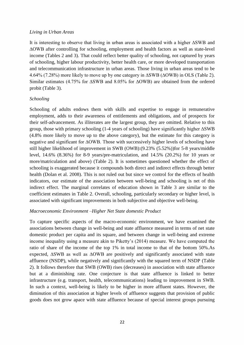
respondent. As shown below in Figure 1, the curve does not show any age pattern except a
sharp plunge among 50-60 years old and then a gradual fall among the oldest (70 years +). It
should be noted that the U shaped curve often derived in the literature reviewed in Section 2
(e.g., Blanchflower and Oswald, 2007) has been derived for the relationship between the level

12
Note: SWB denotes the change in subjective economic well-being. Source: Authors’ computations.
of SWB and age. Hence we do not expect the U-shaped or the inverted U-shaped in the
relationship between ∆SWB and age.
4. Models
We have employed multiple regression and ordered probit models. Their salient features are
described below.
(1) Multiple Regression Model
We first estimate a multiple regression model where the dependent variable, ∆SWB (0, 1, 2),
corresponding to ‘worse-off’, ‘just the same’ or ‘better-off’- are estimated by a set of
explanatory variables using OLS.12 The explanatory variables include the age of the
household head and its squared term, log per capita expenditure in the initial year13, and the
ratio of per capita expenditure of the household to the maximum value in the primary
sampling unit (PSU). The last variable captures the relative consumption level of the
household compared to the richest household within a village (or a corresponding
geographical unit). The model also controls for demographic characteristics such as gender of
the household head, caste, marital status, and religion. To reflect the structure of the economy
and society between urban and rural areas, we include a dummy variable on whether a
household is in a rural or urban area. Also, we include the variables on employment in terms
12See Angrist and Pischke (2008) for the detailed argument in favour of the Linear Probability Model
(LPM) over the probit model where OLS is used for a binary choice model, against the standard textbook
recommendation for the use of probit or logit models for the binary variable. The use of OLS for the
discrete variable (0, 1, 2) can be justified on the same grounds. OLS with robust clustered standard errors
is used to address possible correlations among individuals within a household as well as heteroscedasticity. 13As Kahneman and Deaton (2010) point out, psychologists and sociologists often plot measures of
subjective well-being against income in dollars, but a strong argument can be made for the logarithm of
income as the preferred scale. The logarithmic transformation represents a basic fact of perception known
as Weber’s Law, which applies generally to quantitative dimensions of perception and judgment (e.g., the
intensity of sounds and lights). The rule is that the effective stimulus for the detection and evaluation of
changes or differences in such dimensions is the percentage change, not its absolute amount.
1
1.05
1.1
1.15
1.2
1.25
1.3
1.35
20 25 30 35 40 45 50 55 60 65 70 75 80
S
WB
Age
Figure 1 The relation between SWB and Age in India
13
of both participation and duration. Other important factors are health or disability conditions.
We include dummy variables on (i) whether a household member suffered from NCD, and
(ii) whether there was a disabled member. Other covariates are whether there was a conflict
in the village, exposure to mass media by gender, whether any household member
experienced a theft and whether received remittances. The model also controls for the net
state-level domestic product per capita and its squared term, and the Piketty measure of
income inequality (i.e., the ratio of share of top 1% to that of bottom 50% in total income).
Because ∆SWB is the perceived change of economic well-being during the last 7 years or
between 2005 and 2012, all the explanatory variables are based on the survey questions in
2005 to partially address the issue of reverse causation from ∆SWB to, for instance, health or
income/expenditure.
In another specification, ∆SWB, a dependent variable, is replaced by ∆OWB (0, 1, 2), which
indicates ‘worse-off’, ‘roughly the same’ or ‘better-off’ based on the ranking of the growth of
real per capita household expenditure and with the frequency distribution identical to ∆SWB.
A standard OLS model is expressed as:
𝑦𝑖 = 𝑋𝑖𝛽 + 𝜀𝑖 ……. (1)
where 𝑦𝑖 is a vector, ∆SWB or ∆OWB (0, 1, 2), the change in subjective or objective well-
being from 2005 to 2012, and 𝑖 stands for the household head (1, …., 27,958). 𝑋𝑖 denotes a
matrix containing the intercept and a number of explanatory variables described above and
𝛽is a vector of coefficients to be estimated. 𝑋𝑖includes household characteristics (such as
age, log of expenditure per capita in 2005,religion, caste, gender, location, household size,
whether suffering from an NCD, a disability, whether experiences a theft, whether receives a
remittance, and whether adult men and women are exposed to mass media in 2005.𝑋𝑖 also
includes the Piketty measure of inequality at the state level (ratio of share of the top 1 % in
total income to that of the bottom 50 %) in 2005. 𝜀𝑖 isa vector of the error term assumed to be
independent and identically distributed. We have applied the Huber–White robust standard
errors to address the heteroscedasticity as 𝑦𝑖 is a discrete measure. As noted earlier, our
application of the standard robust OLS to a discrete dependent variable is justified on the
grounds of a well-known argument where robust OLS performs well for the binary dependent
variable (Angrist and Pischke, 2008).
(2) Ordered Probit
As a robustness check, we have applied the ordered probit as well, as the dependent variable
is an ordered discrete variable. It has two merits: it yields separate estimation of the three
cases of ∆SWB or ∆OWB - whether worse-off or just the same or better-off between 2005
and 2012. Also, the prediction of the OLS model can be outside the range between 0 and 2,
though we are not using the predictions in our study. Once we convert the coefficients to
marginal effects/associations evaluated at means, the estimates are fully comparable between
OLS and ordered-probit. More specifically, the coefficient estimates of OLS are equivalent to
the average differences of marginal effects/associations for the three cases.

14
In the probit model, the inverse standard normal distribution of the probability is modelled as
a linear combination of the predictors. The ordered probit (OP) model is a generalization of
the probit model to the case of more than two outcomes of an ordinal dependent variable (a
dependent variable for which the potential values have a natural ordering, as in worse-off,
just the same, and better off).
To avoid repetition, we present below an algebraic exposition of a basic ordered probit model
(Greene, 2018). Let us begin with a latent variable specification.
𝑦𝑖∗ = 𝑥𝑖𝛽′ + 𝑒𝑖
𝑦𝑖∗ is unobserved. What we do observe is
𝑦𝑖 = 0 if 𝑦𝑖∗ ≤ 0
𝑦𝑖 = 1 if 0 < 𝑦𝑖∗ ≤ 𝜇
𝑦𝑖 = 2 if 𝜇 < 𝑦𝑖∗
𝜇is an unknown parameter to be estimated with 𝛽′. The respondents have their own
preferences which depend on certain measurable factors, represented by 𝑥𝑖, such as age,
gender, and income/expenditure, and some unmeasurable factors distributed independently of
the observed factors. The essential ingredient is the mapping from an underlying, naturally
ordered preference scale to a discrete ordered observed outcome in terms of the perceived
change in the economic well-being, or ∆SWB. Given only three possible answers, the
respondents choose the cell that most closely represents their preferences (Greene, 2018).
It is assumed that 𝑒𝑖 is normally distributed. The mean and variance are normalised to be zero
and one, respectively. With the normal distribution, the following probabilities are obtained:
𝑃𝑟𝑜𝑏(𝑦𝑖 = 0) = Φ(−𝛽′𝑥𝑖)
𝑃𝑟𝑜𝑏(𝑦𝑖 = 1) = Φ(Φ(𝜇 − 𝛽′𝑥𝑖) − 𝛽′𝑥𝑖) − Φ(−𝛽′𝑥𝑖)
𝑃𝑟𝑜𝑏(𝑦𝑖 = 2) = 1 − Φ(𝜇 − 𝛽′𝑥𝑖)
In order for all probabilities to be positive, it must be 𝜇>0. The marginal effects/associations
are different from the ordered probit (OP) regression coefficients. Both the sign and
magnitude of marginal effects vary with the ordered outcome. As Greene (2018) offers a
detailed account of how the marginal effects are calculated, we have refrained from an
exposition here. There are mainly two ways of calculating the marginal effects. The first is to
derive the marginal effects for all the explanatory variables in 𝑥𝑖for each observation (for i=1,
…., 27,958) and take the averages for each explanatory variable. The second is to compute
the marginal effect corresponding to each coefficient for a particular explanatory variable by
assuming that all the other explanatory variables take the mean values. We have applied both
methods, but we primarily focus on the results of the latter as this is directly comparable to
the OLS estimates. We carry out the Wald test which examines the linear restrictions 𝛽1 = 𝛽2
= ⋯ .𝛽𝑗−1 or H0: 𝛽𝑞 – 𝛽1 =0 ,q= 2, . . . , J – 1.

15
5. Results
(a) Descriptive Statistics
The list of variables and their means and standard deviation are given in Table 1.
Table 1: List of Variables and Descriptive Statistics
Variable Mean Std. Dev. Min Max
SWB 1.292 0.634 0 2
Monthly Per capita expenditure (’00) 8.442 8.23 0.04 392.73
Household per capita expenditure as fraction of highest in PSU 0.456 0.268 0.004 1
Gender
Female 0.078 0.268 0 1
Marital Status
Unmarried 0.008 0.091 0 1
Widowed/Divorced 0.099 0.299 0 1
Age 45.926 12.406 16 97
Household Size
1 0.007 0.082 0 1
>5 0.374 0.484 0 1
Sector
Urban 0.311 0.463 0 1
Education
1-4 0.117 0.322 0 1
5-8 0.236 0.425 0 1
9-10 0.170 0.376 0 1
>10 0.129 0.335 0 1
Religion
Muslim 0.108 0.310 0 1
Others 0.061 0.239 0 1
Caste
Brahmin 0.050 0.217 0 1
High Caste 0.154 0.361 0 1
Dalit 0.221 0.415 0 1
Adivasi 0.081 0.273 0 1
Others 0.130 0.336 0 1
Household remittance
Yes 0.067 0.250 0 1
Any Work
< 240Hrs 0.111 0.314 0 1
Number of Working Adults (20-50) males in HH
0 0.248 0.432 0 1
>=2 0.076 0.264 0 1
Number of Working Adults (20-50) Females in HH
1 0.465 0.499 0 1
>=2 0.027 0.161 0 1
NCD

16
Yes 0.087 0.281 0 1
Disability
Yes 0.031 0.173 0 1
Radio regular Men
Regularly 0.143 0.350 0 1
Radio regular Women
Regularly 0.120 0.325 0 1
Newspaper regular Men
Regularly 0.201 0.401 0 1
Newspaper regular Women
Regularly 0.105 0.307 0 1
TV regular Men
Regularly 0.349 0.477 0 1
TV regular Women
Regularly 0.411 0.492 0 1
Social Networks
1 0.187 0.390 0 1
2 0.105 0.307 0 1
>2 0.071 0.257 0 1
Theft
Yes 0.047 0.212 0 1
Conflict in village
Yes 0.477 0.500 0 1
Ratio of share top 1% to bottom 50% 0.465 0.119 0.226 0.858
Net State domestic Product (in ‘000) 23.631 9.391 7.914 63.877
Notes: (i) Number of obs = 27,958; (ii) Source: Computed from IHDS
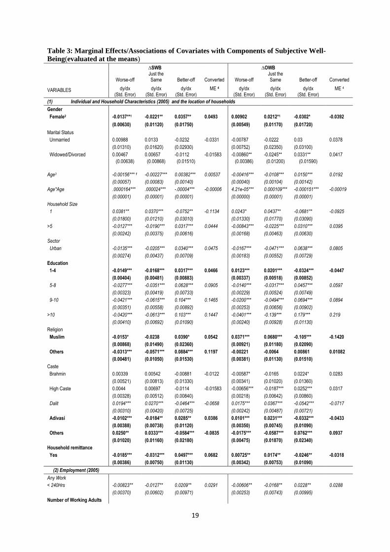
Tables 2 and 3 report the coefficient estimates of the OLS model and the marginal
effects/associations (evaluated at the means) of ordered probit respectively.14It is noted that
we have converted the coefficient estimates to the marginal effects/associations evaluated at
the means in Table 3 so that the OP results in Table 3 are comparable with the OLS results in
Table 2 after a simple conversion. For instance, the first row of Table 3 in the case of ∆SWB
shows that ‘being a female household head’ leads to a change of the probability in the case of
‘Worse Off (0)’ by ‘-1.37%’, that for ‘Just the Same (1)’ by ‘-2.21%’ and that for ‘Better Off
(2)’ by ‘3.57%’ while other covariates are fixed at their means. That is, being a female head
on average leads to a 4.93% (=-1.37%*0+ (-2.21%)*1+ 3.57%*2) increase in the probability
of shifting to the one above category. This is comparable with the OLS estimate of “0.0486”
(4.86%) in the first row of Table 2. All the estimates in Table 2 and Table 3 are highly similar
after this conversion. The probabilities of moving up by one category are shown as
‘Converted ME (Marginal Effect)’ in the last columns of Table 3 for both ∆SWB and ∆OWB.
We follow Angrist and Pischke’s (2008) defence of the use of OLS for the binary dependent
variable. As a robustness check, we have applied an alternative method of deriving the
marginal effects for the ordered probit model by averaging marginal effects for all the
observations (Appendix Table A2). The converted marginal effects are highly similar to those
14All marginal effects are significant at the ≤10 % level unless stated otherwise.

17
in Table 3 and the coefficient estimates in Table 2 (OLS). These three sets of results strongly
corroborate the robustness of OLS in case it is applied to the discrete dependent variable.
Below we discuss the results of these tables together with a particular focus on distinct
differences of the covariates of ∆SWB and ∆OWB. In Table 2 (OLS), although the null of
homoscedasticity is not rejected, we report robust OLS results in Table 2 given that the
dependent variable is discrete for both ∆SWB and ∆OWB. The overall explanatory power of
the specification is validated by the F test in both cases. In Table 3 the overall validation of
the OP specification is confirmed by the Wald test. As in the multiple regression analysis, the
components of well-being are for 2012 and most covariates for 2005.
Table 2 Multiple Regression Analysis of Subjective and Objective Well-Being and Its Covariates
∆SWB ∆OWB
VARIABLES Coefficient Robust Std. Err Coefficient Robust Std. Err
(1) Individual and Household Characteristics and the location of households (2005)
Gender Female 0.0486 (0.0328) -0.0315 (0.0269) Marital Status Unmarried -0.0315 (0.0446) 0.0371 (0.0501) Widowed/Divorced -0.0145 (0.0292) 0.0356 (0.0250) Age3 0.00535** (0.00251) 0.0184*** (0.00305) Age*Age -5.66e-05** (2.60e-05) -0.000186*** (3.29e-05) Household Size 1 2 -0.115*1 (0.0604) -0.0793 (0.0613) >5 0.0438*** (0.0121) 0.0410*** (0.0105) Sector Urban 0.0464*** (0.0118) 0.0728*** (0.0106) Education 1-4 0.0480*** (0.0181) -0.0415*** (0.0159) 5-8 0.0923*** (0.0145) 0.0552*** (0.0127) 9-10 0.146*** (0.0172) 0.0836*** (0.0145) >10 0.145*** (0.0198) 0.202*** (0.0176) Religion Muslim 0.0552 (0.0386) -0.130*** (0.0353) Others 0.118*** (0.0267) 0.00638 (0.0237) Caste Brahmin -0.0114 (0.0226) 0.0187 (0.0213) High Caste -0.0153 (0.0155) 0.0266* (0.0137) Dalit -0.0664*** (0.0154) -0.0678*** (0.0130) Adivasi 0.0391* (0.0207) -0.0359* (0.0201) Others -0.0830** (0.0368) 0.0847** (0.0337) Household remittance Yes 0.0673*** (0.0261) -0.0345 (0.0219)
(2) Employment (2005)
Any Work < 240Hrs 0.0305* (0.0185) 0.0290* (0.0164) Number of Working Adults (20-50) males in HH 0 -0.0874*** (0.0150) 0.0481*** (0.0127) >=2 0.0510*** (0.0187) -0.142*** (0.0160) Number of Working Adults (20-50) Females in HH 1 0.00927 (0.0119) 0.00308 (0.0103) >=2 0.0367 (0.0298) -0.102*** (0.0272)
(3) Health & Disability (2005)
NCD Yes -0.0371* (0.0204) 0.0239 (0.0163) Disability Yes -0.0743*** (0.0284) -0.0347 (0.0229)
(4) Media Access (2005)
Radio regular Men Regularly 0.0954*** (0.0252) -0.0109 (0.0226) Radio regular Women Regularly -0.0508* (0.0278) 0.00732 (0.0239) Newspaper regular Men Regularly 0.0565*** (0.0186) 0.0211 (0.0151)

18
Newspaper regular Women Regularly 0.0404** (0.0201) 0.108*** (0.0177) TV regular Men Regularly -0.00981 (0.0175) -0.00216 (0.0159) TV regular Women Regularly 0.0563*** (0.0176) 0.0314** (0.0157)
(5) Other Variables (2005)
Social Networks 1 0.00994 (0.0149) -0.0152 (0.0127) 2 -0.0469*** (0.0175) -0.0120 (0.0148) >2 0.00267 (0.0182) 0.00385 (0.0173) Theft Yes -0.0269 (0.0255) -0.0643*** (0.0212) Conflict in village Yes 0.0163 (0.0105) -0.0373*** (0.00929)
(6) Initial Economic Conditions (2005)
Monthly Per capita expenditure (’00) 0.00449*** (0.00117) -0.0463*** (0.00269) Square of Monthly Per capita expenditure (’00) -2.38e-05** (1.02e-05) 0.000204*** (3.89e-05) Household per capita expenditure as fraction of highest in PSU
0.0685*** (0.0258) -0.249*** (0.0252)
Ratio of share top 1% to bottom 50% 0.261*** (0.0364) -0.0670** (0.0332) Net State domestic Product (in ‘000) 0.00738*** (0.00201) 0.0120*** (0.00176) Net State domestic Product (in ‘000) Square -7.77e-05** (3.09e-05) -0.000133*** (2.68e-05) Constant 0.736 (0.0639) 1.124 (0.0776) Observations 27,958 27,945 R-squared 0.063 0.223
Notes: 1. Robust Standard errors in parentheses. *** p<0.01, ** p<0.05, * p<0.1.; 2. The results where the coefficient estimates are statistically significant for ∆SWB and ∆OWB with an opposite sign, or only significant for ∆SWB are highlighted in bold; 3. The results where the coefficient estimates are statistically significant for ∆SWB and ∆OWB with a same sign are highlighted in Italics.
We will first focus on the coefficient estimates which show similar patterns in the results, that
is, the common covariates of ∆SWB and ∆OWB (for which the results are given in italics in
Tables 2 and 3).We will then discuss the explanatory variables which are statistically
significant and show opposite signs for ∆SWB and ∆OWB, or significant only for ∆SWB in
Table 2 and Table 3 to identify the correlates specific to ∆SWB (indicated in bold in Tables).
Finally, we will selectively mention a few other coefficient estimates, that is, those which are
statistically significant (or not significant) for either ∆SWB or ∆OWB.15 Only select cases are
highlighted below due to the space constraint.
15Throughout the study, we use the terms, such as associations or marginal effects, given that ∆SWB or
∆OWB in 2005-2012 is regressed on the variables in 2005 following the convention, for instance, of the
empirical studies on macroeconomic growth using cross-country data. We note that for ∆SWB, though it is
based on the survey data in 2012, and the reference point is 2005, a few variables on economic status on
the right hand side are not strictly exogenous, but the reverse causality is reasonably rejected. ∆OWB can
also be influenced by the initial economic status, but, as noted earlier, it is crucial for the initial economic
status to be controlled for in order to interpret ∆OWB as the well-being change after controlling for the
initial differences in OWB. The possibility of reverse causality is ruled out for other covariates. We have
avoided using an IV model as it is highly sensitive to the choice of an instrument, which would make the
comparisons of the estimates for ∆SWB and ∆OWB difficult.
19
Table 3: Marginal Effects/Associations of Covariates with Components of Subjective Well-
Being(evaluated at the means)
∆SWB ∆OWB
Worse-off
Just the Same Better-off Converted Worse-off
Just the Same Better-off Converted
VARIABLES dy/dx (Std. Error)
dy/dx (Std. Error)
dy/dx (Std. Error)
ME 4
dy/dx (Std. Error)
dy/dx (Std. Error)
dy/dx (Std. Error)
ME 4
(1) Individual and Household Characteristics (2005) and the location of households
Gender
Female2 -0.0137**1 -0.0221** 0.0357** 0.0493 0.00902 0.0212*1 -0.0302* -0.0392
(0.00630) (0.01120) (0.01750) (0.00549) (0.01170) (0.01720)
Marital Status
Unmarried 0.00988 0.0133 -0.0232 -0.0331 -0.00787 -0.0222 0.03 0.0378
(0.01310) (0.01620) (0.02930) (0.00752) (0.02350) (0.03100)
Widowed/Divorced 0.00467 0.00657 -0.0112 -0.01583 -0.00860** -0.0245** 0.0331** 0.0417
(0.00638) (0.00868) (0.01510) (0.00386) (0.01200) (0.01590)
Age3 -0.00156*** 1 -0.00227*** 0.00382*** 0.00537 -0.00416*** -0.0108*** 0.0150*** 0.0192
(0.00057) (0.00083) (0.00140) (0.00040) (0.00104) (0.00142)
Age*Age .0000164*** .000024*** -.00004*** -0.00006 4.21e-05*** 0.000109*** -0.000151*** -0.00019
(0.00001) (0.00001) (0.00001) (0.00000) (0.00001) (0.00001)
Household Size
1 0.0381** 0.0370*** -0.0752** -0.1134 0.0243* 0.0437** -0.0681** -0.0925
(0.01800) (0.01210) (0.03010) (0.01330) (0.01770) (0.03090)
>5 -0.0127*** -0.0190*** 0.0317*** 0.0444 -0.00843*** -0.0225*** 0.0310*** 0.0395
(0.00242) (0.00375) (0.00616) (0.00168) (0.00463) (0.00630)
Sector
Urban -0.0135*** -0.0205*** 0.0340*** 0.0475 -0.0167*** -0.0471*** 0.0638*** 0.0805
(0.00274) (0.00437) (0.00709) (0.00183) (0.00552) (0.00729)
Education
1-4 -0.0149*** -0.0168*** 0.0317*** 0.0466 0.0123*** 0.0201*** -0.0324*** -0.0447
(0.00404) (0.00481) (0.00883) (0.00337) (0.00518) (0.00852)
5-8 -0.0277*** -0.0351*** 0.0628*** 0.0905 -0.0140*** -0.0317*** 0.0457*** 0.0597
(0.00323) (0.00419) (0.00733) (0.00229) (0.00524) (0.00749)
9-10 -0.0421*** -0.0615*** 0.104*** 0.1465 -0.0200*** -0.0494*** 0.0694*** 0.0894
(0.00351) (0.00558) (0.00892) (0.00253) (0.00656) (0.00902)
>10 -0.0420*** -0.0613*** 0.103*** 0.1447 -0.0401*** -0.139*** 0.179*** 0.219
(0.00410) (0.00692) (0.01090) (0.00240) (0.00928) (0.01130)
Religion
Muslim -0.0153* -0.0238 0.0390* 0.0542 0.0371*** 0.0680*** -0.105*** -0.1420
(0.00868) (0.01490) (0.02360) (0.00921) (0.01180) (0.02090)
Others -0.0313*** -0.0571*** 0.0884*** 0.1197 -0.00221 -0.0064 0.00861 0.01082
(0.00481) (0.01050) (0.01530) (0.00381) (0.01130) (0.01510)
Caste
Brahmin 0.00339 0.00542 -0.00881 -0.0122 -0.00587* -0.0165 0.0224* 0.0283
(0.00521) (0.00813) (0.01330) (0.00341) (0.01020) (0.01360)
High Caste 0.0044 0.00697 -0.0114 -0.01583 -0.00656*** -0.0187*** 0.0252*** 0.0317
(0.00328) (0.00512) (0.00840) (0.00218) (0.00642) (0.00860)
Dalit 0.0194*** 0.0270*** -0.0464*** -0.0658 0.0175*** 0.0367*** -0.0542*** -0.0717
(0.00310) (0.00420) (0.00725) (0.00242) (0.00487) (0.00721)
Adivasi -0.0102*** -0.0184** 0.0285** 0.0386 0.0101*** 0.0231*** -0.0332*** -0.0433
(0.00388) (0.00738) (0.01120) (0.00350) (0.00745) (0.01090)
Others 0.0250** 0.0333*** -0.0584*** -0.0835 -0.0175*** -0.0587*** 0.0762*** 0.0937
(0.01020) (0.01160) (0.02180) (0.00475) (0.01870) (0.02340)
Household remittance
Yes -0.0185*** -0.0312*** 0.0497*** 0.0682 0.00725** 0.0174** -0.0246** -0.0318
(0.00386) (0.00750) (0.01130) (0.00342) (0.00753) (0.01090)
(2) Employment (2005)
Any Work
< 240Hrs -0.00823** -0.0127** 0.0209** 0.0291 -0.00606** -0.0168** 0.0228** 0.0288
(0.00370) (0.00602) (0.00971) (0.00253) (0.00743) (0.00995)
Number of Working Adults

20
(20-50) males in HH
0 0.0273*** 0.0344*** -0.0617*** -0.089 -0.0104*** -0.0309*** 0.0414*** 0.0519
(0.00348) (0.00393) (0.00736) (0.00191) (0.00601) (0.00790)
>=2 -0.0135*** -0.0244*** 0.0379*** 0.0514 0.0412*** 0.0664*** -0.108*** -0.1496
(0.00371) (0.00734) (0.01100) (0.00459) (0.00499) (0.00937)
Number of Working Adults (20-50) Females in HH
1 -0.00243 -0.00352 0.00595 0.00838 -0.000887 -0.00234 0.00323 0.00412
(0.00246) (0.00356) (0.00602) (0.00169) (0.00446) (0.00615)
>=2 -0.0101 -0.0157 0.0259 0.0361 0.0285*** 0.0531*** -0.0816*** -0.1101
(0.00658) (0.01100) (0.01760) (0.00675) (0.00921) (0.01590)
(3) Health & Disability (2005)
NCD
Yes 0.0116*** 0.0155*** -0.0271*** -0.0387 -0.00614** -0.0171** 0.0232** 0.0293
(0.00428) (0.00525) (0.00952) (0.00253) (0.00752) (0.01000)
Disability
Yes 0.0239*** 0.0287*** -0.0527*** -0.0767 0.00803 0.0189* -0.0270* -0.0351
(0.00755) (0.00739) (0.01490) (0.00496) (0.01060) (0.01560)
(4) Media Access
Radio regular Men
Regularly -0.0259*** -0.0445*** 0.0704*** 0.0963 0.00275 0.00695 -0.0097 -0.01245
(0.00425) (0.00861) (0.01280) (0.00359) (0.00884) (0.01240)
Radio regular Women
Regularly 0.0162*** 0.0211*** -0.0373*** -0.0535 -0.0018 -0.00475 0.00655 0.00835
(0.00600) (0.00702) (0.01300) (0.00364) (0.00980) (0.01340)
Newspaper regular Men
Regularly -0.0167*** -0.0265*** 0.0432*** 0.0599 -0.00564** -0.0153** 0.0209** 0.0265
(0.00361) (0.00625) (0.00984) (0.00257) (0.00727) (0.00983)
Newspaper regular Women
Regularly -0.0136*** -0.0218*** 0.0354*** 0.0490 -0.0229*** -0.0771*** 0.1000*** 0.1229
(0.00440) (0.00773) (0.01210) (0.00238) (0.01010) (0.01240)
TV regular Men
Regularly 0.00286 0.00412 -0.00698 -0.00984 0.000896 0.00232 -0.00321 -0.0041
(0.00418) (0.00597) (0.01020) (0.00287) (0.00740) (0.01030)
TV regular Women
Regularly -0.0160*** -0.0238*** 0.0398*** 0.0558 -0.00760*** -0.0200*** 0.0276*** 0.0352
(0.00401) (0.00609) (0.01010) (0.00279) (0.00745) (0.01020)
(5) Other Variables (2005)
Social Networks
1 -0.00294 -0.00446 0.0074 0.01034 0.00375* 0.00948* -0.0132* -0.01692
(0.00281) (0.00431) (0.00712) (0.00206) (0.00507) (0.00713)
2 0.0146*** 0.0190*** -0.0336*** -0.0482 0.00236 0.00608 -0.00844 -0.0108
(0.00400) (0.00475) (0.00874) (0.00257) (0.00646) (0.00903)
>2 -0.000267 -0.000394 0.000661 0.000928 -0.000733 -0.00197 0.0027 0.00343
(0.00436) (0.00646) (0.01080) (0.00298) (0.00806) (0.01100)
Theft
Yes 0.00797 0.0109 -0.0188 -0.0267 0.0163*** 0.0353*** -0.0516*** -0.0679
(0.00544) (0.00695) (0.01240) (0.00433) (0.00774) (0.01200)
Conflict in village
Yes -0.00490** -0.00713** 0.0120** 0.01687 0.00877*** 0.0226*** -0.0314*** -0.0402
(0.00221) (0.00324) (0.00545) (0.00157) (0.00397) (0.00552)
(6) Initial Economic Conditions (2005)
Monthly Per capita expenditure
-0.00126*** -0.00183*** 0.00309*** 0.00435 0.0103*** 0.0267*** -0.0370*** -0.0473
(0.00023) (0.00034) (0.00056) (0.00027) (0.00056) (0.00064)
Household per capita expenditure as fraction of highest in PSU
-0.0203*** -0.0294*** 0.0497*** 0.0700 0.0509*** 0.132*** -0.183*** -0.2340
(0.00481) (0.00700) (0.01180) (0.00345) (0.00881) (0.01200)
Ratio of share top 1% to bottom 50%
-0.0790*** -0.115*** 0.194*** 0.273 0.0146** 0.0379** -0.0524** -0.0669
(0.00983) (0.01400) (0.02370) (0.00661) (0.01730) (0.02390)
Net State domestic Product -0.00107*** -0.00155*** 0.00262*** 0.00369 -0.00132*** -0.00343*** 0.00475*** 0.00607

21
(in ‘000)
(0.00014) (0.00021) (0.00035) (0.00010) (0.00026) (0.00036)
Notes: 1. Standard errors in parentheses. *** p<0.01, ** p<0.05, * p<0.1. 2.; 2. The results where the coefficient estimates are statistically significant for ∆SWB and ∆OWB with an opposite sign, or only significant for ∆SWB are highlighted in bold. Significance judged by a subset of three marginal effects/associations at the 10% level; 3. The results where the coefficient estimates are statistically significant for ∆SWB and ∆OWB with the same sign are highlighted in italics. Significance judged by a subset of three marginal effects/associations at the 10% level; 4. Average ME (marginal effects) show the additional probability that a household shifts to the category (0,1,2) one above and this is equivalent to the OLS estimate in Table 2. This is equal to ‘0*ME for “0” + 1*ME for “1” + 2*ME for “2”’.
(a) Common Covariates of ∆SWB and ∆OWB
Age with a Non-linear effect
The coefficient of age is positive and significant while that of square of age is negative and
significant for both ∆SWB and ∆OWB in OLS (Table 2).This is consistent with the ordered
probit results where age is negatively associated with being worse-off and just the same and
positively with being better-off for ∆SWB and ∆OWB (Table 3). Households with an old
head tend to feel their economic well-being has improved both subjectively and objectively,
with the association attenuating as the head gets older. If a head gets one year older, the
household is more likely to move to one above category of ∆SWB (or ∆OWB) by 0.54% (or
1.84%) on average, other things being equal (Table 2). This is consistent with marginal
effect/association estimates in Table 3 (0.537% (or 1.92%)). The association of age with the
improvement in well-being is thus much larger for OWB than for SWB.
Household Size
Living arrangements can be associated with perceived change in well-being. These are
captured through the household size. As households with 2-5 persons are the largest group,
this group is omitted. So relative to this group, those living alone are associated with lower
∆SWB and ∆OWB and those belonging to households with more than 5 members express a
higher ∆SWB and ∆OWB in OLS (Table 2). Given the weak social security system, and
weakening family ties, it is not surprising that living alone is closely associated with lower
well-being and belonging to large households (> 5 members) with higher ∆SWB or ∆OWB.
In addition to economies of scale in household consumption expenditure, the joy of living
with children, and perhaps better family support during contingencies (e.g., accident and
serious illness) influences the results on ∆SWB and ∆OWB. So ‘insurance’ against
misfortunes and other contingencies underlie this result. For instance, compared with the
default household size (2-5), a larger household (>5) tends to see the probability of
perceiving a better economic well-being (by one category) increase by 4.38% for ∆SWB and
4.10% for ∆OWB. Consistent results are found in Table 3 in terms of the sign and magnitude
of marginal effects/associations (4.44% for ∆SWB and 3.96% for ∆OWB). In Table 3, for
both ∆SWB and ∆OWB, relative to the omitted group of households with 2-5 members, those
living alone are more likely to be worse-off and just the same and less likely to be better-off,
while those living in households with > 5 members are less likely to be worse-off and just the
same and more likely to be better-off. Not only the signs but also the magnitude of the
associations are similar for both ∆SWB and ∆OWB.
22
Living in Urban Areas
It is interesting to observe that living in urban areas is associated with a higher ∆SWB and
∆OWB after controlling for schooling, employment and health factors as well as state-level
income (Tables 2 and 3). That could reflect better quality of schooling, not captured by years
of schooling, higher labour productivity, better health care, or more developed transportation
and telecommunication infrastructure in urban areas. Those living in urban areas tend to be
4.64% (7.28%) more likely to move up by one category in ∆SWB (∆OWB) in OLS (Table 2).
Similar estimates (4.75% for ∆SWB and 8.05% for ∆OWB) are obtained from the ordered
probit (Table 3).
Schooling
Schooling of adults endows them with skills and expertise to engage in remunerative
employment, adds to their awareness of entitlements and obligations, and of prospects for
their self-advancement. As illiterates are the largest group, they are omitted. Relative to this
group, those with primary schooling (1-4 years of schooling) have significantly higher ∆SWB
(4.8% more likely to move up to the above category), but the estimate for this category is
negative and significant for ∆OWB. Those with successively higher levels of schooling have
still higher likelihood of improvement in SWB (OWB):(9.23% (5.52%))for 5-8 years/middle
level, 14.6% (8.36%) for 8-9 years/pre-matriculation, and 14.5% (20.2%) for 10 years or
more/matriculation and above) (Table 2). It is sometimes questioned whether the effect of
schooling is exaggerated because it compounds both direct and indirect effects through better
health (Dolan et al. 2008). This is not ruled out but since we control for the effects of health
indicators, our estimate of the association between well-being and schooling is net of this
indirect effect. The marginal correlates of education shown in Table 3 are similar to the
coefficient estimates in Table 2. Overall, schooling, particularly secondary or higher level, is
associated with significant improvements in both subjective and objective well-being.
Macroeconomic Environment –Higher Net State domestic Product
To capture specific aspects of the macro-economic environment, we have examined the
associations between change in well-being and state affluence measured in terms of net state
domestic product per capita and its square, and between change in well-being and extreme
income inequality using a measure akin to Piketty’s (2014) measure. We have computed the
ratio of share of the income of the top 1% in total income to that of the bottom 50%.As
expected, ∆SWB as well as ∆OWB are positively and significantly associated with state
affluence (NSDP), while negatively and significantly with the squared term of NSDP (Table
2). It follows therefore that SWB (OWB) rises (decreases) in association with state affluence
but at a diminishing rate. One conjecture is that state affluence is linked to better
infrastructure (e.g. transport, health, telecommunications) leading to improvement in SWB.
In such a context, well-being is likely to be higher in more affluent states. However, the
diminution of this association at higher levels of affluence suggests that provision of public
goods does not grow apace with state affluence because of special interest groups pursuing

23
their own agenda and diverting public resources to their own interests. Table 2 and Table 3
have similar results.
(b) Specific Covariates of ∆SWB
While the correlates of ∆SWB and those of ∆OWB are generally similar and consistent, there
are some factors associated with only ∆SWB as delineated below.
Being a Female Head of Household
We find by ordered probit model that women (i.e. female heads of household) are less likely
to be worse-off and just the same but more likely to be better- off (∆SWB) with significant
marginal effects/associations with a higher probability (4.93% on average) of moving up by
one category (Table 3).This is surprising, especially in light of robust evidence of
discrimination against women in allocation of food and medical resources (e.g., Kynch and
Sen, 1983). However, the signs are reversed and the corresponding probability is -3.92 (Table
3). While the signs are the same, the coefficient estimates are not significant when OLS is
applied to ∆SWB or ∆OWB (Table 2).
Religion
Another important variable is religion. As Hindus are the largest group, it is omitted. Relative
to this group, ‘Muslims’ and ‘Others’ (including those belonging to Jainism and Buddhism)
tend to have higher ∆SWB, while Muslims tend to have lower ∆OWB (Table3). Three
observations are pertinent: Hinduism is different from many religions because it has no
specific beliefs that everyone must agree with to be considered a Hindu. Instead, it is
inclusive of many different, sometimes contradictory, beliefs. For example, hidden within
Hinduism are both theistic and semi-theistic schools or philosophies. Moreover, the caste
system is integral to Hinduism. As the former is divisive and exclusionary, Hindus as a
religious group are likely to have lower ∆SWB. The third observation is a pervasive view that
belief in God helps imbibe values of forbearance, integrity and compassion (Dolan et al. 2008
and Deaton, 2011). These values are reinforced by, say, regular church attendance or
performance of rituals or, more broadly, religiosity (Helliwell, 2003). It is noted that Muslims
or ‘Others’ tend to perceive improved subjective well-being without experiencing
corresponding improvement in objective-well-being. In particular, the lower ∆OWB among
Muslims reflects that they are on average more deprived than Hindus.
Caste
The caste hierarchy reveals a somewhat intriguing pattern. As OBCs are the largest group, it
is omitted. Relative to this group, the highest ranking Brahmins do not display a significantly
higher well-being (either ∆SWB or ∆OWB), while those belonging to High Castes have a
significantly higher level of well-being (only ∆OWB, Table 2). Dalits/SCs, who are on the
lower rung, are, however, associated with significantly lower ∆SWB and ∆OWB in Table 2
(based on robust regression). However, Table 3 (based on OP) shows that their probability of
moving up rises in both ∆SWB and ∆OWB by 6.58% (7.17%). Adivasis/STs, who are on the
lowest rung, display a significantly higher well-being for ∆SWB (by 3.91%), but the sign is

24
reversed for ∆OWB (-3.56%) as shown in Table 2, with similar estimates (3.86%; -4.33%) of
marginal correlates as given in Table 3. The residual category of ‘Others’ shows a
significantly lower well-being for ∆SWB with the opposite sign for ∆OWB. The fact that
there is little consonance between caste hierarchy and well-being - particularly SWB -
suggests that the latter has little to do with poverty. To illustrate, while Dalits and Adivasis
are most likely to be poor, their subjective well-being differs. In contrast, while Brahmins are
least likely to be poor, their subjective well-being is not significantly higher than OBCs’.16
Employment
We also include the variables on whether employed as well as the duration of employment.
The first variable shows the number of adult male and female workers in the household,
respectively. The number of workers in the age-group 20-50 years is classified into the three
categories, ‘0’, ‘1’, ‘2 or more’. As households with 1 adult male worker are the largest
group, this is omitted. Relative to this group, households without any male worker are
associated with lower ∆SWB and those with ‘2 or more’ adult male workers with higher
∆SWB, but the signs are reversed for ∆OWB (Tables 2 and 3). Since households without any
adult female worker are the largest group, this is the omitted group. Relative to these
households, those with ‘2 or more’ adult female workers are associated with lower ∆OWB,
but it is not significant in the case of ∆SWB (Tables2 and 3). The coefficient/marginal effect
of households with a single worker is positive but not significant (Tables 2 and 3). Duration
of employment is not sufficiently disaggregated for meaningful inferences. There are just two
categories: ‘annual hours worked ≤ 240 hours’ and ‘> 240 hours’. The first category lumps
together those who hardly any work with those who work 20 hours or less in a month. The
difficulty is that the threshold for the leisure-work choice cannot be identified. As households
with workers exceeding 240 hours are more numerous, these are omitted. Relative to this
group, those working ≤ 240 hours display higher ∆SWB and ∆OWB. This is counter-
intuitive.
NCDs
Change in SWB and ill-health or disabilities are likely to be negatively associated. We use
two relevant indicators: one is non-communicable diseases (NCDs) and the second is
disabilities/limitations of ADL. Their separate roles suggest that NCDs or disabilities are
significantly associated with lower well-being, relative to those not suffering from either,
respectively. The reverse causality where high SWB lowers prospects of ill-health is
minimised as ill-health (in 2005) is prior to well-being (in 2012). Though our SWB measure
is the perceived change of economic well-being in 2005-2012, it is ruled out that the
perception in 2012 influences ill-health in 2005. In any case, as observed by Kohler et al.
(2017), the causality from health to well-being is more likely.
If an individual in a household suffers from any NCD, the household is more likely to be
worse-off and just the same and less likely to be better-off, relative to those not suffering
from any NCD only for ∆SWB, not ∆OWB (Tables 2 and 3).Similar results are obtained for
16For a definitive assessment based on rural samples from select north-Indian states, see Spears (2016).

25
individuals suffering from any disability only for ∆SWB, not for ∆OWB (Table 2). More
specifically, households with disabled are more likely to be worse-off and just the same and
less likely to be better-off in terms of SWB (Table 3).
Mass-media
The association between SWB and exposure to mass-media has not received much attention.
IHDS allows us to examine this relationship in detail. The mass media include radio,
newspapers and TV. Exposure of men and women is classified into ‘never’, ‘sometimes’ and
‘regularly’. By combining ‘never’ and ‘sometimes’, we are able to focus on regular exposure
of men and women separately and their associations with ∆SWB and ∆OWB. For men, well-
being and regular exposure to radio and newspapers but not TV are positively related,
implying that they perceive a positive change in SWB. These factors are not significantly
associated with ∆OWB (Tables 2 and 3). In sharp contrast, women reading newspapers and
watching TV experience greater improvement in both subjective and objective well-being
(Tables 2 and 3). However, regular listening to radio by women is not associated with ∆SWB
or ∆OWB. Overall, the results corroborate the importance of exposure to mass-media -
particularly for women in improving SWB.
Initial Consumption
The relationship between change in subjective well-being and income remains controversial
with some studies reporting a positive relationship and others a varying relationship,
depending on the region (Kahneman and Deaton, 2010). Following Deaton (2011), we use
the log of per capita expenditure as a proxy for the log of per capita income. Our results show
a positive and significant relation between ∆SWB and initial expenditure, implying the higher
the initial expenditure, the higher is change in SWB, with the probability of moving up by
one category as 0.45% (Table 2). The corresponding estimate is 0.44% in Table 3. However,
the sign is reversed as higher initial expenditure reduces the growth rate of per capita
consumption.17
(c) Other Covariates of ∆SWB and ∆OWB
Remittances
As remittances include international transfers mostly from non-resident relatives and
acquaintances, they are in a large number of cases an important supplement to household
income/expenditure (Imai et al. 2014). As expected, these are associated with higher ∆SWB,
but not ∆OWB (Table 2). Households receiving remittances are less likely to be worse-off
and just the same and more likely to be better-off, relative to those who do not in the case of
∆SWB, but not in the case of ∆OWB (Table 3).
17 Admittedly, the variables on the initial per capita household expenditure are likely to be endogenous, but
we include them in estimating ∆OBW to facilitate the comparison of the results for ∆SWB and ∆OWB.
Omitting the initial expenditure, its square and its share in PSU from the equation estimating ∆OBW does
not significantly affect the estimates of other coefficients except that estimates for schooling in the top two
categories become statistically non-significant.

26
Other Covariates
Marital status is found to be closely linked to SWB-in particular, the married are found to
enjoy higher SWB (Helliwell, 2003). IHDS allows us to disaggregate marital status into:
married, unmarried, separated and divorced. As ‘the married’ is the largest category, this is
omitted. Neither unmarried nor widowed and divorced show significant differences in terms
of ∆SWB or ∆OWB (Tables 2 and 3). It is important to bear in mind that married women do
not enjoy improvement in their subjective or objective well-being. This may seem counter-
intuitive, but is not because many of the married women are subject to intimate partner
violence including marital ‘rape’.
There are frequent conflicts in the local neighbourhood, some minor and others not minor and
on a larger scale. Inter-caste conflicts (e.g., rape of a Dalit woman), disputes over ownership
of land or property, and communal riots vary in scale and intensity. Relative to no conflict,
conflicts are associated with a significantly lower well-being changes for ∆OWB (Tables2
and 3). For ∆SWB conflict is statistically non-significant in Table 2 but positive and
significant in Table 3. The latter seems counter-intuitive, as even minor conflicts involve loss
of property, loss of income and violence. Another variable of interest is crimes. IHDS is
confined to thefts. Thefts are not significantly associated with ∆SWB but are significantly
and negatively associated with ∆OWB (Tables 2 and 3). A definitive result would have been
obtained if the value of stolen items were given.
Participation in social networks such as self-help groups, women’s associations, and
producers’ associations is potentially beneficial during illness, loss of livelihood, and other
contingencies such as accidents and the death of the primary bread winner (Dolan et al. 2008;
Birkman et al. 2012; Deaton 2018). However, in the absence of information on density of
these networks and people’s frequency of participation, their importance in enhancing SWB
may be inconclusive. There are four categories of participation in networks: 0, 1, 2 and > 2.
As households not affiliated to any social network are the largest group, it is omitted. So
relative to this group, the only significant positive association is between change in ∆SWB
and ∆OWB and households belonging to 2 networks (Table 2). However, in Table 3 the signs
are reversed which is counter-intuitive.
Piketty (2014) drew attention to growth in developed countries over a long period leading to
a rise in income inequality. In another study, Chancel and Piketty (2017) point to a rise in
income inequality in India since 1922. The important contribution of these studies is to shift
the attention away from conventional measures of income inequality (say, the Gini
coefficient) to income disparity between the top 1 % and the bottom 50 %. We find that the
association between well-being and the Piketty measure of extreme income inequality is
positive and significant. This suggests that the higher the ratio of share of the top 1% in total
income to that of the bottom 50 %, the higher is ∆SWB. This is counter-intuitive as the
income accumulation of multi-millionaires is driven by speculative gains in the stock market
and real estate.

27
6. Discussion and Policy Challenges
Although there is abundant literature on SWB, there is virtually none for India18. Growing
recognition of the validity and accuracy of measures of SWB vis-à-vis objective measure of
well-being (based on real income) underlies the rapid growth of literature on SWB in recent
decades. As prominent studies in the SWB literature, such as Deaton (2018), Kahneman and
Krueger (2006), Kahneman and Deaton (2010), Blanchflower and Oswald, (2007), and
Diener et al. (2013), among others, have emphatically endorsed the case for SWB both
conceptually and empirically, and drawn attention to its policy importance, we were
motivated to examine the relationship between SWB and its covariates in the Indian context.
However, our measure of SWB relates to changes and is confined to perceived economic
well-being. Hence, arguably our analysis is both more challenging and more innovative.
Furthermore, we identified the household-level covariates of the perceived changes in SWB
in comparison with the changes in OWB, objective well-being, in the same period. To our
knowledge, this has not been studied in the SWB literature.
IHDS contains a measure of the perceived change of economic well-being at the household
level compared with 7 years ago. Admittedly narrow, our SWB measure has advantages over
the standard scale measures in econometric modelling because of its simplicity (e.g. being
less subject to heterogeneity among different individuals in the level of their aspirations, or
perception/interpretation of the survey questions on the scale of happiness). The measure is
associated with income and related measures but also with other individual characteristics
such as age, caste, religion, living arrangements, schooling, media exposure and state
affluence and extreme income inequality. Hence this measure of well-being captures more
than what is anticipated or implied by conventional measures of economic well-being. This
imparts policy significance to analysis such as ours. As a broad statement, our discussion of
the significance of the results highlights the importance of the context, model specifications
and their implementation.
First, common factors associated with both ∆SWB and ∆OWB have been identified. We have
found that larger households with an old (70 years and above) and highly schooled head,
located in urban areas or affluent states in 2005 tended to experience further improvement in
both SWB and OWB in 2005-2012.
From a life-cycle perspective, the relationship between SWB and age has received
considerable attention. Some have reported a U-shaped SWB-age curve in Britain and USA
(e.g., Blanchflower and Oswald, 2007), and others (notably, Deaton, 2018) report a U-shaped
relationship in English speaking countries, and absence of an age pattern in low-income
countries in Africa and South Asia. A few studies have reported an inverted U-shape in the
USA (e.g., Easterlin, 2006). Our multiple regression analysis confirms a non-linear
relationship between ∆SWB and age, with a positive coefficient of age and a negative
coefficient of square of age. A similar relation is found for the relationship between ∆OWB
and age. A graphical illustration of the relationship between the predicted ∆SWB and age is
18With the exception of Spears (2016) which is confined to rural areas in select north-Indian states.
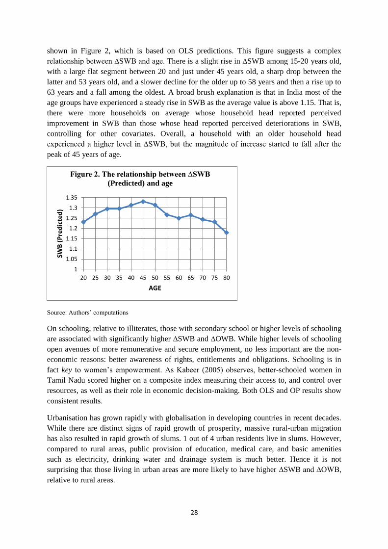
28
shown in Figure 2, which is based on OLS predictions. This figure suggests a complex
relationship between ∆SWB and age. There is a slight rise in ∆SWB among 15-20 years old,
with a large flat segment between 20 and just under 45 years old, a sharp drop between the
latter and 53 years old, and a slower decline for the older up to 58 years and then a rise up to
63 years and a fall among the oldest. A broad brush explanation is that in India most of the
age groups have experienced a steady rise in SWB as the average value is above 1.15. That is,
there were more households on average whose household head reported perceived
improvement in SWB than those whose head reported perceived deteriorations in SWB,
controlling for other covariates. Overall, a household with an older household head
experienced a higher level in ∆SWB, but the magnitude of increase started to fall after the
peak of 45 years of age.
Source: Authors’ computations
On schooling, relative to illiterates, those with secondary school or higher levels of schooling
are associated with significantly higher ∆SWB and ∆OWB. While higher levels of schooling
open avenues of more remunerative and secure employment, no less important are the non-
economic reasons: better awareness of rights, entitlements and obligations. Schooling is in
fact key to women’s empowerment. As Kabeer (2005) observes, better-schooled women in
Tamil Nadu scored higher on a composite index measuring their access to, and control over
resources, as well as their role in economic decision-making. Both OLS and OP results show
consistent results.
Urbanisation has grown rapidly with globalisation in developing countries in recent decades.
While there are distinct signs of rapid growth of prosperity, massive rural-urban migration
has also resulted in rapid growth of slums. 1 out of 4 urban residents live in slums. However,
compared to rural areas, public provision of education, medical care, and basic amenities
such as electricity, drinking water and drainage system is much better. Hence it is not
surprising that those living in urban areas are more likely to have higher ∆SWB and ∆OWB,
relative to rural areas.
1
1.05
1.1
1.15
1.2
1.25
1.3
1.35
20 25 30 35 40 45 50 55 60 65 70 75 80
SWB
(P
red
icte
d)
AGE
Figure 2. The relationship between ∆SWB
(Predicted) and age

29
The macro context is significant too. Two aspects are considered. One is state affluence
measured through NSDP per capita and its square. The second is the Piketty measure of
extreme income inequality. As expected, the relationship between ∆SWB or ∆OWB and state
affluence is positive and significant. We have also found that the relationship between ∆SWB
or ∆OWB and the square of NSDP per capita is negative and significant. It follows therefore
that well-being rises in association with state affluence but at a diminishing rate. One
conjecture is that state affluence is linked to better infrastructure (public health,
transportation, and telecommunication) and schooling quality. In such a context, well-being is
likely to be higher in more affluent states. However, the diminution of this association at
higher levels of affluence suggests that provision of public goods does not grow apace with
state affluence because of special interest groups pursuing their own agenda and/or
diminishing marginal effects of public goods. Besides, while lobbying is inevitable, it is not
clear how to regulate it or, who regulates the regulator (Stigler, 1971).
Secondly, we have identified the factors significantly associated with ∆SWB, but not ∆OWB.
We have found that households with a female household head, more male members in the
labour market, with regular exposure to mass media, without members suffering from non-
communicable diseases or disability are more likely to be better- off subjectively without
experiencing corresponding improvement in OWB.
Relative to men, women are more likely to perceive a better change in SWB. Available
evidence points to women being better-off in specific contexts (Deaton, 2011, 2018, Dolan et
al. 2008, among others). However, women in India-especially in the north- are subject to
widespread abuse, violence and discrimination in employment. It is thus highly improbable
that they enjoy higher well-being unless there is diminution of abuse and violence (Kulkarni
et al. 2013).
Religion is important.. While Dolan et al. (2008) is an early review of evidence on religion
and its practice, Deaton (2011, 2018) offer a richer and more insightful review of the
relationship between ∆SWB, religion and religiosity. Our analysis is confined to the
relationship between change in well-being and major religious groups. Relative to Hindus,
Muslims and Others (belonging to Jainism, Buddhism) are less likely to be worse-off and just
the same and more likely to be better-off. The OLS results are similar in as much as change
in SWB is significantly higher among these religions. Two observations are pertinent. One is
that Hinduism has no specific beliefs that must be adhered to by every Hindu. Instead, it is
inclusive of many different beliefs of which some are contradictory (e.g., hidden within
Hinduism are both theistic and semi-theistic philosophies). Besides, in Hinduism today there
exists, on the one hand, faith in the efficacy of ritual and desire for its worldly fruits and, on
the other, disregard for all external practices and material results (Encyclopaedia Britannica,
2021). On the broader question of why religion matters is that belief in God enables the
followers to be calm, generous, sensitive to pain and suffering of others and helps imbibe the
virtues of integrity and forbearance (Dolan et al. 2008, Deaton, 2011, 2018). That this is not
entirely true is manifested by communal riots except that more often than not these are
caused by miscreants. Maintaining religious harmony is thus essential.

30
Inherent in the caste-system is a socio-economic hierarchy, with Brahmins and High Castes at
the top and SCs/Dalits and STs/Adivasis at the bottom. Inter-caste marriages are abhorred
and, despite affirmative action (reservations in schools and colleges, and public employment),
the fate of lower castes has not significantly improved. Discrimination against lower castes in
employment is rampant as the legislation against discrimination is largely ineffective
(Deshpande, 2013). So the associations between improvement in perceived well-being
(∆SWB) and caste are not in consonance with the hierarchy. In comparison with OBCs (a low
caste group but higher ranked than Dalits and Adivasis), Brahmins do not display a
significantly higher increase in SWB. SCs/Dalits display a significantly higher ∆SWB and
∆OWB while STs/Adivasis record a significant positive relationship with respect to ∆SWB
and a negative relationship to ∆OWB19. Others - a mixed but more affluent group- show a
significantly lower ∆SWB. It is thus implied that poverty and well-being do not necessarily
move in tandem.
Another income-related variable is employment. The larger the number of adult male workers
in a household, the greater is improvement in SWB, but not OWB. It has been emphasised
that short-term unemployment is not so demoralising as longer-term unemployment. We are
unable to test this hypothesis. However, as noted in the previous two sub-sections, the
estimates of duration of employment /hours worked in a year are not sufficiently
disaggregated to identify number of hours at which work-leisure choice occurs. In any case,
available evidence for other developing countries is mixed (Dolan et al. 2008).
Chronic diseases and disabilities have long-lasting effects. Stroke, osteoporosis, cancer,
mental disorder, vision impairment, difficulty in walking, and dressing not only act as
impediments to remunerative employment but also are a financial burden on the family.
Besides, it is demeaning to be dependent on others in carrying out activities of daily living.
So it is not surprising that a negative association between SWB and ill-health across different
regions and countries is observed (e.g., Deaton 2011, 2018). Data constraints restricted our
analysis to 4 major NCDS: hypertension, cardio-vascular diseases, diabetes and cancer and
change in SWB. However, the coverage of disabilities or limitations of ADL is more
detailed. Our results confirm a robust negative relationship between lower ∆SWB and NCDs
in both OLS and OP results, but this is not found for ∆OWB. An equally robust negative
association is observed between lower ∆SWB and disabilities, but this is not found for
∆OWB. Whether individuals adjust to disability is confirmed in a few studies (Dolan et al.
2008, Deaton, 2018). Due to the lack of data on adaptation to disabilities, we are unable to
throw new light.
Exposure of men and women to mass media highlights the role of information in
improvement in well-being. The results are striking. Mass media access is particularly
important for improvement in SWB, but not much in OWB. For men, there is a significant
positive association between ∆SWB and regular exposure to radio and newspapers but not
TV. While women listening regularly to radio do not show a higher ∆SWB, those regularly
reading newspapers and watching TV experience higher ∆SWB. Only women’s regular
19The results vary with the specification. These are the findings based on the OP analysis.
31
access to radio significantly improved OWB. Does information content vary from one
medium to another? Do men and women react differently to news coverage of, say, rapes,
sexual harassment, violence against women, high food prices, health risks and mortality?
These questions can only be answered through a more detailed investigation which is not
feasible with IHDS. So, a common presumption that wider dissemination of information is
necessarily a good thing is not consistent with our findings. More attention to its content is
necessary. While self-regulation by the media has not been successful, there is a real risk that
government intervention may suppress freedom of expression.
On the relationship between income/consumption and SWB, our literature review in Section
2 points to a divergence in the empirical evidence. As documented in Deaton (2018) and
others, either the two are unrelated or there is a positive relationship, with the magnitude
varying by region and even with the same data. We find that there is a robust positive
relationship between ∆SWB and log of per capita expenditure in the initial year. This is not
found for ∆OWB.
Finally, we have examined in detail whether other factors are associated with ∆SWB by
including them as covariates in OLS and ordered probit models.
Whether SWB and marital status are linked has been widely studied, with the evidence
favouring the married (e.g., Deaton, 2018, Diener et al. 2013, Dolan et al. 2008, among
others). However, our multiple regression results do not show a significant difference in
change in subjective well-being between the unmarried, or the widowed/divorced, relative to
the married. These are plausible findings as married women are subject to intimate partner
violence-including marital ‘rape’, discrimination in intra-household allocation of food and
resources for medical care and restrictions on ‘outside’ employment.
The significant positive relationship between ∆SWB and the Piketty measure of extreme
income inequality is intriguing-especially when the income gains of millionaires and
billionaires are driven by speculative gains in the stock market and real estate. This is what
Chancel and Piketty (2017) demonstrated with their meticulous research of income tax
records and other sources in India. If their portfolio is more diversified and labour intensive,
it cannot be ruled out that the income gains will be more widely distributed. At the same
time, vigorous promotion of micro, small and medium enterprises/MSMEs is likely to expand
employment and generate income on a large-scale. In contrast, a significantly negative
association is found between ∆OWB and the Piketty measure.
A major limitation of our analyses is that with just two waves of the panel data in IHDS we
are unable to capture household heterogeneity through experiments with random and fixed
effects. This may be feasible when the third wave of IHDS is available,
Thanks to the important contributions of Sen (1985) and Deaton’s (2018) emphasising in
different ways a broadening of the focus for assessing well-being-specifically, looking
beyond per capita income as a measure-there is growing consensus that perceptions of well-
being matter a great deal. Although our analysis of change in SWB is narrowly focused on
perceived change in economic well-being, its comparison with changes in OBW yields

32
important insights into the commonalities and divergences between them. For example, the
lack of consonance between the socio-economic hierarchy and change in SWB is revealing.
While Brahmins are at the top of this hierarchy, they fare worse than the lower rungs
comprising SCs and STs in this measure of well-being. Despite their greater vulnerability to
poverty and other deprivations, they are more likely to move up the ranks of ∆SWB. To
borrow Sen’s powerful terminology, this is compatible with these deprived groups’ better
functioning (eg, easier access to education, healthcare). As Deaton emphasised, in a similar
vein, measures such as SWB may enable individuals to live better lives while policy makers
design and implement appropriate policies.
Although some policy concerns are briefly referred to in the preceding discussion, a more
integrated perspective is delineated below.
As income and its growth are closely related to improvement in SWB, a fiscal stimulus that
generates incomes through strengthening of infrastructure-roads, transportation, power
generation, irrigation, schools, and hospitals is a priority. But there are challenges within
these components. Whether the state alone can finance massive investment in infrastructure is
doubtful. Public-private partnerships are key but an environment that promotes such
partnerships –while the public sector designs these interventions and commits financially in
the MOU, incentives in the form of assured returns must be provided for the private sector.
At the same time, regulation by the public sector must not stifle private participation through
avoidable bureaucratisation.
To illustrate challenges for public policies within specific areas, a few examples suffice.
Positive externalities of building roads in rural areas-especially those that do not get washed
away during the monsoon-are likely to be greater than building highways and strengthening
inter-city connectivity. Limited allocations to solar energy development and continued heavy
reliance on thermal energy are lop-sided given high levels of pollution and rising incidence
of respiratory ailments and certain types of cancer such as breast, liver, and pancreatic, and
high risk of mortality. In irrigation, as opposed to large-scale projects, higher priority should
be given to small-scale projects that pool local water resources (ponds, streams) and are
shared equitably through community networks (Wade, 1988). A substantial increase in public
investment for schooling is of course imperative but alongside greater attention must be given
to upgrading its quality. Rampant absenteeism of teachers, their lack of training, shortage of
text books, and absence of toilets for female students to which pointed attention was drawn
by Sen and Dreze (1995) are still as relevant and cry out for reform. A National Health Policy
was announced in 2017. It proposed raising public health expenditure progressively to 2.5%
of the GDP by 2025 and advocated a major chunk of resources to primary health care,
followed by secondary and tertiary health care. This policy together with the NITI Aayog
action agenda have set targets for reduction of premature death and morbidity due to major
NCDs in India. There are two serious concerns, however. One is that scant attention is given
to where the resources will come from. Another glaring omission is that little is said about the
rapid rise in the share of the old in the total population and associated multi-morbidities of
NCDs. Besides, continuing neglect and failure to anticipate these demographic and
epidemiological shifts-from infectious diseases to NCDs-may result in enormously costlier

33
policy challenges (Jan et al. 2018, Bloom et al. 2020). Given the rapid deterioration in the
quality of public healthcare and rising life expectancy and expectations of good quality health
care, the supply - demand imbalance is likely to widen sharply. So a priority is to increase
substantially expenditure on health. But more important than higher financial allocation is
reorganisation of the health care system and effective regulation. As argued emphatically in
an important study (Patel et al. 2015), it is imperative to develop a fully integrated
population-based healthcare system that brings together the public and private sectors and the
allopathic and indigenous systems, and is well-coordinated at different levels of service
delivery platforms-primary, secondary and tertiary. Moreover, a case is made for a shift from
a standard health insurance model to an entitlement-based model.
India enacted the Rights of Persons with Disabilities Act, 2016 (the “New Act”) and the rules
thereunder (the “Rules”) in 2017. The New Act replaced the Persons with Disabilities (Equal
Opportunity Protection of Rights and Full Participation) Act, 1995 (the ‘previous Act’),
which covered only seven disabilities. The New Act covers more than 15 disabilities
including dwarfism, acid attack victims, intellectual disability and specific learning
disabilities. It defines a ‘person with disability’ as someone with long term physical, mental,
intellectual or sensory impairment which, in interaction with barriers, hinders his / her full
and effective participation in society equally with others.
Yet discrimination persists in various forms - in employment, access to financial services,
health services-specifically, against women, elderly and tribal communities (Kulkarni et al.
2020).
Behavioural changes are no less important and perhaps also no less challenging. A few
important contributions using evidence from LMICs and from India yield useful insights
(Gaiha et al. 2020). Inadequate physical activity and unbalanced high-calorie diets promote
weight gains. Obesity is a risk factor for cardiovascular and diabetes and can aggravate
symptoms of CVD such as emphysema and bronchitis (Academy of Medical Sciences, 2018).
Limiting tobacco consumption is expected to benefit at the individual level but wider
reduction in multi-morbidity prevalence requires taxation on unhealthy products. For
example, there is evidence that tobacco taxation reduces smoking and such benefits might
also lead to a reduction in certain multi-morbidity clusters (Sassi et al. 2018). It is reassuring
therefore that taxation of beedis and smokeless tobacco (SLT) has risen sharply in the recent
Goods and Services Tax (GST).
Information through mass-media adds to awareness of healthy living, entitlements, social
safety nets, and discriminatory behaviour. While the links between improvement in well-
being and mass-media vary between men and women, it is plausible that some information
content is more offensive to women. That self-censorship by the media has been shrouded in
corruption is common knowledge while government regulation is oversensitive to any
criticism and frequently authoritarian. It is thus a challenge that defies any resolution.
The socio-economic hierarchy inherent in the caste system is not reflected in change in SWB.
Indeed, relative to OBCs, upper castes do not display significantly higher changes in SWB

34
while among SCs on the lower rung change in well-being is significantly higher. Despite
affirmative action, caste inequities and discrimination against lower castes have persisted.
While a case could be made for lower castes catching up with upper castes though more
equitable opportunities of schooling, employment and personal advancement, it is arguable
that upper castes might resent it unless their attitudes towards lower castes change drastically.
As legislation has limited potential because of weak enforcement, it has been argued that,
since mere exhortations to change attitudes are likely to be ignored, carefully framed
persuasion can work. For instance, people conform to others they perceive to be in their
reference group. These effects are quite powerful messages that are framed to appeal to self-
interest or moral commitments usually lead to less behavioural (and attitude) change than
those that are framed to make the recipients believe that others just like them are behaving in
the desired way. For example, rates of tax compliance go up, and deductions go down, when
citizens believe other citizens are paying their fair share (Bilz and Nadler, 2014).
The fact that Muslims and Others, relative to Hindus, are associated with higher levels of
improvement in SWB is not surprising as Hinduism is ‘more a way of life than a religion’. It
lacks a code of beliefs and religious practices are flexible. Moreover, the caste system- an
integral part of Hinduism- is iniquitous and exclusionary. Religious harmony is vital for
improvements in SWB.
Inequality in income/wealth distribution at different levels is yet another challenge, as it is
tied up with incentives to invest and grow. While there is no question about progressive
taxation of inherited wealth, progressive taxation of income is likely to be resisted as it
affects negatively investment behaviour. So the policy challenge is to ensure that the trade-off
between income tax and investment is not unacceptably high. Our analysis suggests that high
disparity between personal incomes within a primary sampling unit (a cluster of
villages/small towns) is linked to the gap between aspiration and achievement and thus
breeds resentment and frustration, and a negative association with well-being. Expansion of
more remunerative employment opportunities may narrow this gap and enhance well-being.
Reduction of disparity in affluence between states through larger allocations of revenues
through the Finance Commission without compromising their incentive to raise more revenue
is an option. But this must be complemented with larger investments by the Centre and state
governments.
Finally, the positive association between well-being and the Piketty measure of extreme
inequality is puzzling especially if the latter is driven mainly by speculative gains in the stock
market and real estate. So there is a case for a more diversified investment portfolio. Whether
speculative gains could be curbed through taxation is moot. Combined with promotion of
small and medium enterprises through tax exemption in the initial phase and easier financing
of their loans could promote more inclusive growth and perhaps substantial gains in SWB.
In brief, there are many policy challenges that are daunting and some that seem unresolvable.

35
References
Academy of Medical Sciences (2018).“Multi-morbidity: A Priority for Global Health
Research,” London.
Akay, A. O. B. Bargain, &H. X. Jara (2017) “Back to Bentham, Should We? Large-Scale
Comparison of Experienced versus Decision Utility”, IZA DP No. 10907, Bonn.
Alesina, A., Di Tella, R., & MacCulloch, R. (2004). Inequality and happiness: Are Europeans
and Americans different? Journal of Public Economics, 88, 2009–2042.
Angrist, J. D., & J. S. Pischke (2008).Mostly harmless econometrics: An empiricist's
companion. Princeton university press, Princeton, NJ:
Berkman, L. F, T V Sekher, B. Capistrant, and Y. Zheng (2012): “Social Networks, Family,
and Care Giving Among Older Adults in India,” Aging in Asia: Findings from New and
Emerging Data Initiatives, J P Smith and M Majmundar (eds), Washington, DC: National
Research Council, pp . 261-278.
Bilz, K., & J. Nadler (2014) “Law, Moral Attitudes, and Behavioural Change”, New York:
Oxford University Press.
Blanchflower, D. G., & Oswald, A. J. (2004). “Well-being over time in Britain and the
USA”.Journal of Public Economics, 88, 1359–1386.
Blanchflower, D.G., & A. Oswald (2007) “Is Well-Being U-Shaped Over The Life Cycle?”,
NBER Working Paper Series, Working Paper 12935, Cambridge, MA.
Bloom, D.E., S. Chen, M.Kuhn, M. E. McGovern, L. Oxley, &K. Prettner (2020) “The
economic burden of chronic diseases: Estimates and projections for China, Japan, and South
Korea”, TheJournal of the Economics of Ageing, forthcoming.
Cantril, H (1965). The pattern of human concerns. New Brunswick, NJ: Rutgers University
Press.
Chancel, L., &T. Piketty. (2017). Indian income inequality, 1922–2014: From British Raj to
Billionaire Raj? WIDER.Working Paper Series, No. 2017/11.
Clark, A. (2003). “Unemployment as a social norm: Psychological evidence from panel
data”. Journal of Labor Economics, 21(2), 323–351.
Clark, A., Frijters, P., & Shields, M. A. (2008).“A survey of the income happiness
gradient”.Journal of Economic Literature.
Clark, A., P. Frijters& M. A. Shields (2008) “Relative Income, Happiness, and Utility: An
Explanation for the Easterlin Paradox and Other Puzzles”, Journal of Economic Literature,
vol. 46, no. 1, March, pp. 95-144.

36
Council for Social Development (2016) Social Development Report: Disability Rights
Perspectives, New Delhi: Oxford University Press.
Deaton, A. (2011) “Aging, Religion, and Health”, D. A. Wise (ed.) Explorations in the
Economics of Aging, University of Chicago Press.
Deaton, A. (2018) “What do self-reports of wellbeing say about life-cycle theory and
policy?”,Journal of Public Economics, 162, 18-25.
Deshpande, A. (2013) Affirmative Action in India, Oxford India Short Introductions, New
Delhi.
Di Tella, R., MacCulloch, &A. Oswald(2001). “Preferences over inflation and
unemployment.Evidence from surveys of happiness”.The American Economic Review, 91(1),
335–341.
Diener, E. R. Inglehart, L. T. (2013)“Theory and Validity of Life Satisfaction Scales”, Soc
Indic Res, 112:497–527.
Dolan, P., T. Peasgood, &M. White (2008) “Do we really know what makes us happy? A
review of the economic literature on the factors associated with subjective well-being”.
Journal of Economic Psychology 29, 94–122.
Dorn, D., J. A. Fischer., G., Kirchgassner,.&A. Sousa-Poza, (2007). “Is it culture of
democracy? The impact of democracy, and culture on happiness”.Social Indicators Research,
82(3), 505–526.
Duesenberry, J. S (1949).Income, Saving and the Theory of Consumer Behaviour.
Cambridge: Harvard University Press.
Easterlin, R. A. (2006). “Life cycle happiness and its sources: Intersections of psychology,
economics, and demography”,Journal of Economic Psychology, 27(4), 463-482.
Encyclopædia Britannica (2021), “Practical Hinduism”, Encyclopædia Britannica, Inc.
Fahey, T., & Smyth, E. (2004). “Do subjective indicators measure welfare? Evidence from 33
European societies”.European Societies, 6(1), 5–27.
Ferrer-i-Carbonell, A. (2005). “Income and well-being: An empirical analysis of the
comparison income effect”. Journal of Public Economics, 89, 997–1019.
Ferrer-i-Carbonell, A., &Gowdy, J. M. (2007).“Environmental degradation and
happiness”.Ecological Economics, 60(3), 509–516.
Gaiha, R., S. Mathur, & Vani S. Kulkarni.(2020). "Rural Poverty and Disability in LMICs."
University of Pennsylvania Population Centre Working Paper (PSC/PARC), 2020-47.
Greene, W. H. (2018) Econometric Analysis, 8th Edition, Pearson India.

37
Haller, M., &M. Hadler, (2006). “How social relations and structures can produce happiness
and unhappiness: An international comparative analysis”. Social Indicators Research, 75,
169–216.
Helliwell, J. F. (2003). “How’s life? Combining individual and national variables to explain
subjective well-being”.Economic Modelling, 20, 331–360.
Imai, K, R. Gaiha, A.Ali,&N. Kaicker. (2014). “Remittances, Growth and Poverty: New
Evidence from Asian Countries”, Journal of Policy Modeling, 36(3), pp. 524-538.
Jan, S. Tracey-Lea Laba, B. M Essue, A. Gheorghe, J. Muhunthan, M. Engelgau, A. Mahal,
U. Griffiths, D. McIntyre, Q. Meng, R. Nugent, &R. Atun (2018) “Action to address the
household economic burden of non-communicable diseases”, Lancet; 391: 2047–58.
Kabeer, N. (2005) “Gender equality and women's empowerment: a critical analysis of the
third Millennium Development Goal”, Gender and Development, Vol. 13, No. 1, March.
Kahneman, D.,& A. B. Krueger (2006) “Developments in the Measurement of Subjective
Well-Being”, Journal of Economic Perspectives—Volume 20, Number 1—Winter—3-2.
Kahneman, D., & A. Deaton (2010) “High income improves evaluation of life but not
emotional well-being”, PNAS | September 21| vol. 107 | no. 38 | 16489–16493.
Kynch, J., and Sen,Amartya (1983) “Indian women: well-being and survival”, Cambridge
Journal of Economics, Vol. 7, No. 3/4 1983), pp. 363-380.
Kohler, I.V., C. F. Payne, C. Bandawe & Hans-Peter Kohler (2017) “The Demography of
Mental Health Among Mature Adults in a Low-Income, High-HIV-Prevalence Context”,
Demography, 54:1529–1558
Kulkarni, Vani S., R. Gaiha and M. Pandey (2013) “MDGs and gender inequality”, BWPI
Woking Paper Series 188, University of Manchester.
Kulkarni, Veena, S. Vani, S. Kulkarni, & R. Gaiha. (2020). "Poverty Transitions, Health, and
Socio-Economic Disparities in India."University of Pennsylvania Population Center Working
Paper (PSC/PARC), 2020-50.
Meier, S. & A. Stutzer. (2006). “Is volunteering rewarding in itself?” Centrefor Behavioural
Economics and Decision-Making, Federal Reserve Bank of Boston.
Mosse, D. (2018) “Caste and development: Contemporary perspectives on a structure of
discrimination and advantage”, World Development,vol. 110, October, pp. 422-436.
Oswald, A. J., & Wu, S. (2010). “Objective confirmation of subjective measures of human
well-being: Evidence from the USA”. Science, 327(5965), 576-579.
Patel, V., R. Parikh, S. Nandraj, P. Balasubramaniam, K. Narayan, V. K Paul, A. K. Shiva
Kumar, M. Chatterjee, &K. Srinath Reddy (2015), “Assuring health coverage for all in
India”, Lancet; 386: 2422–35.

38
Piketty,T. (2014) Capital in the Twenty First Century, Cambridge: Harvard University Press.
Ravallion, M., K. Himelein& K. Beegle (2016) “Can Subjective Questions on Economic
Welfare Be Trusted?”,Economic Development and Cultural Change,volume 64, no. 4.
Ravallion, M. (2014) “Poor, or Just Feeling Poor? On Using Subjective Data in Measuring
Poverty”, In Happiness and Economic Growth, A. Clark and Cl. Senik (eds,) Oxford:
Oxford University Press.
Sassi, F.,A. Belloni, A. J. Mirelman, M. Suhrcke, A. Thomas, N. Salti, S.Vellakkal, C.
Visaruthvong, B. M Popkin, &R.Nugent (2018) “Equity Impacts of Price Policies to Promote
Healthy Behaviours”, Lancet, May 19; 391, 2059–2070.
Sen, Amartya & J. Dreze (1995) India: Economic Development and Social Opportunity,
Oxford: Clarendon Press.
Sen, Amartya (1985) Commodities and Capabilities, Amsterdam, North Holland.
Spears, D. (2016) “Caste and Life Satisfaction in Rural North India”, Economic and Political
Weekly, January 23.
Stigler, G. (1971). “The theory of economic regulation”, Bell J. Econ. Man. Sci. 2:3-21.
Stutzer, A. (2004) “The role of income aspirations in individual happiness”, Journal of
Economic Behavior& Organization, vol. 54, issue 1, 89-109.
Wade,R. (1988) Village Republics: Economic Conditions for Collective Action in South
India, Cambridge: Cambridge University Press.
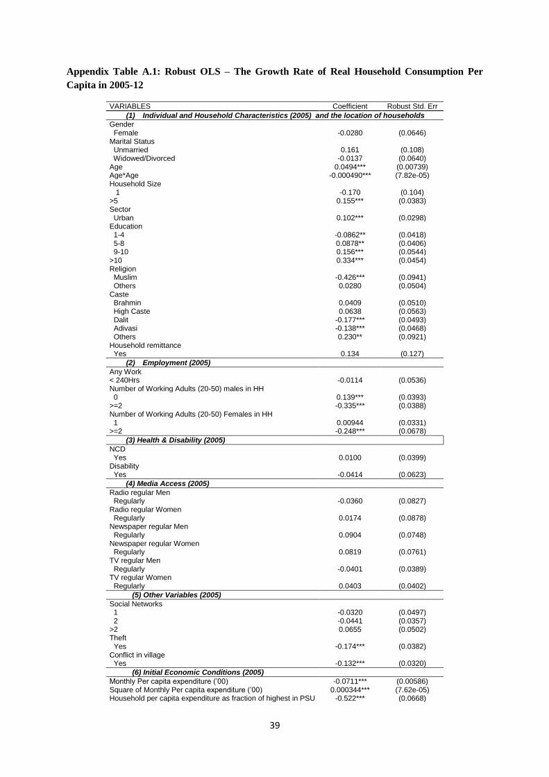
39
Appendix Table A.1: Robust OLS – The Growth Rate of Real Household Consumption Per
Capita in 2005-12
VARIABLES Coefficient Robust Std. Err
(1) Individual and Household Characteristics (2005) and the location of households
Gender Female -0.0280 (0.0646) Marital Status Unmarried 0.161 (0.108) Widowed/Divorced -0.0137 (0.0640) Age 0.0494*** (0.00739) Age*Age -0.000490*** (7.82e-05) Household Size 1 -0.170 (0.104) >5 0.155*** (0.0383) Sector Urban 0.102*** (0.0298) Education 1-4 -0.0862** (0.0418) 5-8 0.0878** (0.0406) 9-10 0.156*** (0.0544) >10 0.334*** (0.0454) Religion Muslim -0.426*** (0.0941) Others 0.0280 (0.0504) Caste Brahmin 0.0409 (0.0510) High Caste 0.0638 (0.0563) Dalit -0.177*** (0.0493) Adivasi -0.138*** (0.0468) Others 0.230** (0.0921) Household remittance Yes 0.134 (0.127)
(2) Employment (2005)
Any Work < 240Hrs -0.0114 (0.0536) Number of Working Adults (20-50) males in HH 0 0.139*** (0.0393) >=2 -0.335*** (0.0388) Number of Working Adults (20-50) Females in HH 1 0.00944 (0.0331) >=2 -0.248*** (0.0678)
(3) Health & Disability (2005)
NCD Yes 0.0100 (0.0399) Disability Yes -0.0414 (0.0623)
(4) Media Access (2005)
Radio regular Men Regularly -0.0360 (0.0827) Radio regular Women Regularly 0.0174 (0.0878) Newspaper regular Men Regularly 0.0904 (0.0748) Newspaper regular Women Regularly 0.0819 (0.0761) TV regular Men Regularly -0.0401 (0.0389) TV regular Women Regularly 0.0403 (0.0402)
(5) Other Variables (2005)
Social Networks 1 -0.0320 (0.0497) 2 -0.0441 (0.0357) >2 0.0655 (0.0502) Theft Yes -0.174*** (0.0382) Conflict in village Yes -0.132*** (0.0320)
(6) Initial Economic Conditions (2005)
Monthly Per capita expenditure (’00) -0.0711*** (0.00586) Square of Monthly Per capita expenditure (’00) 0.000344*** (7.62e-05) Household per capita expenditure as fraction of highest in PSU -0.522*** (0.0668)

40
Ratio of share top 1% to bottom 50% -0.0881 (0.127) Net State domestic Product (in ‘000) 0.0246*** (0.00484) Net State domestic Product (in ‘000) Square -0.000247*** (7.34e-05) Constant -0.126 (0.169) Observations 27,945 R-squared 0.053
Robust Standard errors in parentheses. Appendix Table A.2: Marginal Effects/Associations of Covariates with Components of Subjective Well-
Being (an alternative estimate of marginal effects based on the average marginal effects for all the observations) ∆SWB ∆OWB
Worse-off
Just the Same Better-off Converted Worse-off
Just the Same Better-off Converted
VARIABLES dy/dx (Std. Error)
dy/dx (Std. Error)
dy/dx (Std. Error)
ME 4
dy/dx (Std. Error)
dy/dx (Std. Error)
dy/dx (Std. Error)
ME 4
(1) Individual and Household Characteristics and the Location of Households (2005)
Gender
Female2 -0.0146**1 -0.0195*1 0.0341**1 0.0487 0.00953* 0.0182* -0.0278* -0.0374
(0.00705) (0.01020) (0.01670) (0.00578) (0.01040) (0.01590)
Marital Status
Unmarried 0.0104 0.0117 -0.0221 -0.0325 -0.00854 -0.0188 0.0273 0.0358
(0.01400) (0.01410) (0.02790) (0.00822) (0.02000) (0.02810)
Widowed/Divorced 0.00494 0.00581 -0.0107 -0.01559 -0.00935** -0.0207** 0.0300** 0.0393
(0.00678) (0.00766) (0.01440) (0.00435) (0.01030) (0.01440)
Age 3 -0.00165***1 -0.00200*** 0.00365*** 0.0053 -0.00446*** -0.00921*** 0.0137*** 0.01819
(0.00061) (0.00073) (0.00134) (0.00043) (0.00088) (0.00130)
Age*Age 1.74e-05*** 2.11e-05***
-3.84e-05***
-0.000056 4.51e-05*** 9.31e-05*** -0.000138*** -0.0001829
(0.00001) (0.00001) (0.00001) (0.00000) (0.00001) (0.00001)
Household Size
1 0.0397** 0.0321*** -0.0719** -0.1117 0.0248* 0.0387** -0.0635** -0.0883
(0.01900) (0.01230) (0.02890) (0.01350) (0.01680) (0.02940)
>5 -0.0134*** -0.0168*** 0.0302*** 0.0436 -0.00905*** -0.0193*** 0.0283*** 0.0373
(0.00298) (0.00410) (0.00594) (0.00209) (0.00431) (0.00579)
Sector
Urban -0.0142*** -0.0183*** 0.0326*** 0.0469 -0.0181*** -0.0400*** 0.0581*** 0.0762
(0.00333) (0.00471) (0.00689) (0.00479) (0.00650) (0.00644)
Education
1-4 -0.0155*** -0.0152*** 0.0307*** 0.0462 0.0123*** 0.0181*** -0.0304*** -0.0427
(0.00447) (0.00528) (0.00867) (0.00366) (0.00513) (0.00804)
5-8 -0.0288*** -0.0320*** 0.0608*** 0.0896 -0.0146*** -0.0275*** 0.0420*** 0.0565
(0.00448) (0.00677) (0.00755) (0.00276) (0.00546) (0.00704)
9-10 -0.0440*** -0.0564*** 0.100*** 0.1436 -0.0211*** -0.0425*** 0.0636*** 0.0847
(0.00614) (0.00977) (0.00929) (0.00347) (0.00696) (0.00841)
>10 -0.0439*** -0.0563*** 0.100*** 0.1437 -0.0447*** -0.116*** 0.160*** 0.204
(0.00649) (0.01060) (0.01110) (0.00584) (0.01050) (0.01020)
Religion
Muslim -0.0162* -0.0211 0.0373* 0.0535 0.0380*** 0.0596*** -0.0976*** -0.1356
(0.00940) (0.01370) (0.02260) (0.01020) (0.01260) (0.01980)
Others -0.0335*** -0.0510*** 0.0845*** 0.118 -0.00241 -0.00539 0.0078 0.01021
(0.00669) (0.01090) (0.01460) (0.00419) (0.00951) (0.01370)
Caste
Brahmin 0.0036 0.00482 -0.00842 -0.01202 -0.00638* -0.0139 0.0203* 0.0267
(0.00556) (0.00722) (0.01270) (0.00378) (0.00867) (0.01230)
High Caste 0.00467 0.0062 -0.0109 -0.0156 -0.00714*** -0.0157*** 0.0229*** 0.0301
(0.00354) (0.00460) (0.00803) (0.00253) (0.00555) (0.00779)
Dalit 0.0205*** 0.0239*** -0.0443*** -0.0647 0.0182*** 0.0318*** -0.0500*** -0.0682
(0.00425) (0.00485) (0.00690) (0.00343) (0.00507) (0.00663)
Adivasi -0.0108** -0.0164** 0.0273** 0.0382 0.0106*** 0.0199*** -0.0305*** -0.0411
(0.00431) (0.00693) (0.01080) (0.00390) (0.00664) (0.01010)
Others 0.0264** 0.0294*** -0.0558*** -0.0822 -0.0196*** -0.0489*** 0.0684*** 0.0879
(0.01110) (0.01120) (0.02090) (0.00601) (0.01560) (0.02080)
Household remittance

41
Yes -0.0198*** -0.0277*** 0.0475*** 0.0673 0.00768** 0.0149** -0.0226** -0.0303
(0.00474) (0.00758) (0.01090) (0.00372) (0.00663) (0.01010)
(2) Employment (2005)
Any Work
< 240Hrs -0.00873** -0.0112** 0.0199** 0.0286 -0.00656** -0.0142** 0.0208** 0.0274
(0.00399) (0.00567) (0.00933) (0.00281) (0.00648) (0.00907)
Number of Working Adults (20-50) males in HH
0 0.0286*** 0.0305*** -0.0591*** -0.0877 -0.0114*** -0.0262*** 0.0376*** 0.049
(0.00467) (0.00634) (0.00742) (0.00262) (0.00527) (0.00712)
>=2 -0.0144*** -0.0219*** 0.0363*** 0.0507 0.0415*** 0.0595*** -0.101*** -0.1425
(0.00453) (0.00683) (0.01050) (0.00610) (0.00955) (0.00985)
Number of Working Adults (20-50) Females in HH
1 -0.00257 -0.00311 0.00568 0.00825 -0.000952 -0.002 0.00295 0.0039
(0.00261) (0.00319) (0.00576) (0.00181) (0.00381) (0.00562)
>=2 -0.0108 -0.0139 0.0247 0.0355 0.0292*** 0.0467*** -0.0759*** -0.1051
(0.00717) (0.00994) (0.01680) (0.00740) (0.01010) (0.01520)
(3) Health & Disability (2005)
NCD
Yes 0.0122*** 0.0136*** -0.0259*** -0.0382 -0.00665** -0.0145** 0.0211** 0.0277
(0.00467) (0.00513) (0.00915) (0.00291) (0.00641) (0.00911)
Disability
Yes 0.0251*** 0.0252*** -0.0503*** -0.0754 0.00849 0.0163* -0.0248* -0.0333
(0.00835) (0.00777) (0.01440) (0.00527) (0.00933) (0.01440)
(4) Media Access
Radio regular Men
Regularly -0.0276*** -0.0398*** 0.0674*** 0.095 0.00294 0.00594 -0.00888 -0.01182
(0.00558) (0.00921) (0.01240) -0.00385 -0.00757 -0.0114
Radio regular Women
Regularly 0.0171*** 0.0185*** -0.0356*** -0.0527 -0.00193 -0.00405 0.00598 0.00791
(0.00656) (0.00680) (0.01240) (0.00394) (0.00833) (0.01230)
Newspaper regular Men
Regularly -0.0176*** -0.0239*** 0.0416*** 0.0593 -0.00607** -0.0130** 0.0191** 0.0252
(0.00444) (0.00640) (0.00953) (0.00290) (0.00622) (0.00894)
Newspaper regular Women
Regularly -0.0144*** -0.0195*** 0.0339*** 0.0483 -0.0255*** -0.0646*** 0.0901*** 0.1156
(0.00506) (0.00731) (0.01160) (0.00428) (0.00910) (0.01100)
TV regular Men
Regularly 0.00303 0.00363 -0.00666 -0.00969 0.00096 0.00198 -0.00294 -0.0039
(0.00444) (0.00527) (0.00967) (0.00308) (0.00631) (0.00938)
TV regular Women
Regularly -0.0169*** -0.0214*** 0.0383*** 0.0552 -0.00815** -0.0171*** 0.0252*** 0.0333
(0.00471) (0.00622) (0.00977) (0.00317) (0.00647) (0.00933)
(5) Other Variables (2005)
Social Networks
1 -0.00312 -0.00395 0.00707 0.01019 0.00400* 0.00811* -0.0121* -0.01609
(0.00300) (0.00386) (0.00680) (0.00225) (0.00439) (0.00653)
2 0.0154*** 0.0167*** -0.0321*** -0.0475 0.00253 0.00519 -0.00772 -0.01025
(0.00453) (0.00497) (0.00841) (0.00275) (0.00555) (0.00827)
>2 -0.000282 -0.000349 0.000631 0.000913 -0.00079 -0.00167 0.00246 0.00325
(0.00462) (0.00572) (0.01030) (0.00322) (0.00685) (0.01010)
Theft
Yes 0.00841 0.00959 -0.018 -0.02641 0.0171*** 0.0306*** -0.0477*** -0.0648
(0.00583) (0.00625) (0.01180) (0.00489) (0.00746) (0.01130)
Conflict in village
Yes -0.00519** -0.00631** 0.0115** 0.01669 0.00939*** 0.0193*** -0.0287*** -0.0381
(0.00237) (0.00307) (0.00524) (0.00209) (0.00365) (0.00503)
(6) Initial Economic Conditions (2005)
Monthly Per capita expenditure -0.00136*** -0.00159*** 0.00295***
0.00431 0.0108*** 0.0235*** -0.0343***
-0.0451
(0.00025) (0.00029) (0.00054) (0.00022) (0.00047) (0.00057)

42
Household per capita expenditure as fraction of highest in PSU -0.0214*** -0.0260*** 0.0474***
0.0688 0.0545*** 0.113*** -0.167***
-0.221
(0.00509) (0.00617) (0.01130) (0.00369) (0.00727) (0.01080)
Ratio of share top 1% to bottom 50% -0.0836 -0.101 0.185
0.269 0.0156 0.0323 -0.0479
-0.0635
(0.01030) (0.01240) (0.02260) (0.00711) (0.01470) (0.02180)
Net State domestic Product (in ‘000) -0.00119 -0.00128 0.00247
0.00366 -0.00145 -0.00290 0.00435
0.0058
(0.00016) (0.00017) (0.00032) (0.00011) (0.00021) (0.00032)
Notes: 1. Standard errors in parentheses. *** p<0.01, ** p<0.05, * p<0.1. 2.; 2. The results where the coefficient estimates are statistically significant for ∆SWB and ∆OWB with an opposite sign, or only significant for ∆SWB are highlighted in bold. Significance judged by a subset of three marginal effects at 10% level; 3. The results where the coefficient estimates are statistically significant for ∆SWB and ∆OWB with a same sign are highlighted in Italics. Significance judged by a subset of three marginal effects at 10% level; 4. Average ME (marginal effects) show the additional probability that a household shifts to the category (0,1,2) one above and this is equivalent to the OLS estimate in Table 2. This is equal to ‘0*ME for “0” + 1*ME for “1” + 2*ME for “2”’.