changes in aerosol properties during spring-summer period

HAL Id: hal-00296427https://hal.archives-ouvertes.fr/hal-00296427

Submitted on 1 Feb 2008

HAL is a multi-disciplinary open accessarchive for the deposit and dissemination of sci-entific research documents, whether they are pub-lished or not. The documents may come fromteaching and research institutions in France orabroad, or from public or private research centers.

L’archive ouverte pluridisciplinaire HAL, estdestinée au dépôt et à la diffusion de documentsscientifiques de niveau recherche, publiés ou non,émanant des établissements d’enseignement et derecherche français ou étrangers, des laboratoirespublics ou privés.

Changes in aerosol properties during spring-summerperiod in the Arctic troposphere

A.-C. Engvall, R. Krejci, J. Ström, R. Treffeisen, R. Scheele, O. Hermansen, J.Paatero

To cite this version:A.-C. Engvall, R. Krejci, J. Ström, R. Treffeisen, R. Scheele, et al.. Changes in aerosol properties dur-ing spring-summer period in the Arctic troposphere. Atmospheric Chemistry and Physics, EuropeanGeosciences Union, 2008, 8 (3), pp.445-462. �hal-00296427�

https://hal.archives-ouvertes.fr/hal-00296427

https://hal.archives-ouvertes.fr

Atmos. Chem. Phys., 8, 445–462, 2008www.atmos-chem-phys.net/8/445/2008/© Author(s) 2008. This work is licensedunder a Creative Commons License.

AtmosphericChemistry

and Physics

Changes in aerosol properties during spring-summer period in theArctic troposphere

A.-C. Engvall1, R. Krejci 1, J. Strom2,3, R. Treffeisen4, R. Scheele5, O. Hermansen6, and J. Paatero7

1Department of Meteorology, Stockholm University, Stockholm, 10691, Sweden2Department of Applied Environmental Science – Atmospheric Science Unit, Stockholm University, Stockholm, 10691,Sweden3Norwegian Polar Institute, 9296 Tromsø , Norway4Alfred-Wegener-Institut fur Polar- und Meeresforschung, Telegrafenberg A43, 14473 Potsdam, Germany5Koninklijk Nederlands Meteorologisch Instituut, Postbus201, 3730, AE, De Bilt, The Netherlands6Norsk institutt for luftforskning, Postboks100, 2027 Kjeller, Norway7Finnish Meteorological Institute, P.O.B. 503, 00101 Helsinki, Finland

Received: 13 November 2006 – Published in Atmos. Chem. Phys. Discuss.: 25 January 2007Revised: 26 November 2007 – Accepted: 3 January 2008 – Published: 1 February 2008

Abstract. The change in aerosol properties during the tran-sition from the more polluted spring to the clean summerin the Arctic troposphere was studied. A six-year data setof observations from Ny-Alesund on Svalbard, covering themonths April through June, serve as the basis for the char-acterisation of this time period. In addition four-day-backtrajectories were used to describe air mass histories. The ob-served transition in aerosol properties from an accumulation-mode dominated distribution to an Aitken-mode dominateddistribution is discussed with respect to long-range trans-port and influences from natural and anthropogenic sourcesof aerosols and pertinent trace gases. Our study shows thatthe air-mass transport is an important factor modulating thephysical and chemical properties observed. However, the air-mass transport cannot alone explain the annually repeatedsystematic and rather rapid change in aerosol properties, oc-curring within a limited time window of approximately 10days. With a simplified phenomenological model, which de-livers the nucleation potential for new-particle formation, wesuggest that the rapid shift in aerosol microphysical proper-ties between the Arctic spring and summer is mainly drivenby the incoming solar radiation in concert with transport ofprecursor gases and changes in condensational sink.

1 Introduction

The Arctic’s vulnerable eco- and climate system has becomea focus of the international scientific community during thelast several decades. Recent studies on the Arctic climateshowed that, due to its sensitivity to external perturbations,

Correspondence to: A.-C. Engvall([email protected])

the Arctic could be seen as possible early warning of globalclimate change. Nowadays climate models predict the largestincrease of the annual mean temperature for the Arctic (Has-sol, 2005).

Unlike many other regions, there are very few localhuman-derived sources of air pollution in the Arctic in ad-dition to the metallurgical industry in the Russian Arctic.Therefore, the transport of pollution including aerosols andits gaseous precursors from industrialized mid-latitude re-gions in Europe, Asia, and North America is of great im-portance. It is suspected that interactions between solar ra-diation, high surface albedo, the aerosol particles and cloudsmagnify the radiative impact of atmospheric aerosols in theArctic region (Quinn et al., 2002). Thus, for a given aerosoldistribution, the specific optical impact is most likely in-creased in this high latitude region.

Experiments conducted in the Arctic over the last 40 yearshave mainly focused on the Arctic Haze phenomenon, i.e.layers with enhanced concentrations of aerosols and precur-sor gases in the Arctic troposphere, which is found duringlate winter and spring. This phenomenon was first notedin the literature of Mitchell (1957). Several years later sci-entists showed the seasonality to have a very strong annualvariation with higher loadings of anthropogenic componentsduring late winter and early spring compared to the sum-mer months and that this perturbation of the Arctic atmo-sphere was caused by anthropogenic sources at lower lat-itudes, especially from the Eurasia continent (Rahn, 1981;Barrie, 1986; Heintzenberg, 1989).

Ground-based measurements from the Zeppelin station,Svalbard, and Point Barrow, USA showed that the aerosolloading undergoes a systematic change from spring tosummer (Bodhaine et al., 1981; Bodhaine, 1989; Quinn et

Published by Copernicus Publications on behalf of the European Geosciences Union.

446 A.-C. Engvall et al.: Spring-summer aerosols in the Arctic troposphere

al., 2002; Strom et al., 2003). Results from these stud-ies demonstrated that there is an increase of aged parti-cles, i.e. accumulation-mode particles (particles larger than100 nm) in winter and spring, which are associated with an-thropogenic sources and long-range transport. In summer,this mode is significantly smaller in terms of number den-sity. Smaller sized aerosols, so-called Aitken-mode particles,which range between about 20 and 100 nm, dominate the sizedistribution. At the same time the total particle number den-sity increases.

In this study we will give emphasis on thetransition fromthe more anthropogenic-influenced spring to clean summerconditions. Transport patterns, trace gases, and aerosol mi-crophysics are investigated for the period April through Junefor the years 2000–2005. It will be shown that the transitionfrom “spring-type” aerosol to “summer-type” aerosol occursalmost at the same time from year to year (give or take afew weeks). We have selected different observational data inorder to answer the question if this transition is mainly con-trolled by changes in the transport of pollutants or if it is aneffect of local processes in the Arctic.

2 Air mass trajectories and long-term measurementsfrom the Zeppelin Station

2.1 Air mass trajectories

The model TRAJKS (Stohl et al., 2001) three-dimensionalfour-day-back trajectories provided by the Royal Nether-lands Meteorological Institute (KNMI) were used to studythe link between air mass origin and the aerosol properties.The trajectories were calculated on daily basis at 12:00 UTCin a regular grid centred at Ny-Alesund (79◦ N, 11.9◦ E) forthe period of April through June during the years 2000–2005. The grid contains, besides the point of Ny-Alesund,four additional surrounding points in an almost symmetri-cal grid with sides of about 100 km. Two of the pointsare located over sea (78.5◦ N, 14.5◦ E and 79.5◦ N, 14.5◦ Eand the other two are located over land (78.5◦ N, 9.5◦ E and79.5◦ N, 9.5◦ E). The objective of investigating this grid wasto demonstrate how representative the trajectories to Ny-Alesund are for a larger area of interest and to see possi-ble difference between sea and land areas. Results from thisstudy show that the flow pattern is essentially identical forall five chosen points. Thus for further calculations only thetrajectories calculated for Ny-Alesund (79◦ N, 11.9◦ E) wereused.

Garrett et al. (2002) study the aerosol around clouds in theArctic and found enhanced concentrations of Aitken nucleusabove the cloud tops. It is conceivable that there is a sourceof particles in the FT that are mixed down to the BL. Westudied if there are any systematic differences in air transportbetween the boundary layer (BL) and free troposphere (FT)over the investigated period. The Micro Pulse Lidar (MPL)

operated by the National Institute for Polar Research (NPIR)often show cloud tops around 2000 m altitude (Shiobara etal., 2003). We thus define this altitude as the border be-tween the BL and FT. The so-called level 1 of the MPL data(available through the internet) shows the normalized relativebackscatter signals and this data is solely used in the studyto get a feeling for typical boundary layer heights based oncloud tops. The 1000 m and 5000 m altitudes are then takento represent airflow in the BL and FT, respectively. Notethat the Arctic atmosphere may present several stable lay-ers, and surface inversions are often observed (Tjernstrom,2005). However, we are interested in the layering that con-tains “weather” (clouds and precipitation), which is why weuse the altitude range indicated by the MPL.

2.2 Long-term measurements

The long-term measurements from the Zeppelin station wereused to evaluate temporal variation of the spring-to-summertransition in aerosol properties on a multi-annual basis. TheZeppelin station is located on Mount Zeppelin 474m abovesea level near the community of Ny-Alesund, Svalbard.Given the elevated location of the Zeppelin station, the effectof local particle sources such as sea spray and re-suspensionof dust from Ny-Alesund are strongly reduced. However, oc-casionally the sea salt and dust can contribute significantlyto the total mass of the particles. Wind fields over Sval-bard are complex, due to the topography and surface char-acteristics. Compared to ocean level observation, the effectsof local wind phenomenon, such as katabatic winds, are re-duced at the Zeppelin station. Measurements of chemicaland physical properties at the Zeppelin station are includedin the Cooperative Programme for Monitoring and Evalu-ation of the Long-range Transmission of Air Pollutants inEurope (EMEP) and the Global Atmosphere Watch (GAW)program coordinated by the World Meteorological Organi-zation (http://www.wmo.int). Further information about theinstrumentation and database are summarized at the home-page http://www.emep.int.

In this study we use aerosol data obtained at the station in-cluding number density, size distributions and activity of theradioactive component lead-210 (210Pb). In addition we alsouse sulfur dioxide (SO2) and carbon monoxide (CO) mea-surements to analyse the history and origin of the air masses.Table 1 gives an overview of data availability for the timeperiod of 2000 through 2005 from Zeppelin station used inthe present study. In general the data availability is typicallybetter than 90% complete each year, but some years are notcovered by all variables. Year 2002 has low data coveragefor aerosol microphysics and less than 50% of210Pb data isavailable for year 2004.

The physical properties of the aerosols, such as the totalparticle number density and the size distribution, are pro-vided by the Department of Applied Environmental Science– Atmospheric science unit (ITM) at Stockholm University.

Atmos. Chem. Phys., 8, 445–462, 2008 www.atmos-chem-phys.net/8/445/2008/

http://www.wmo.int

http://www.emep.int

A.-C. Engvall et al.: Spring-summer aerosols in the Arctic troposphere 447

Table 1. Available trace gas- and aerosol data used in this study.

Trace gas Unit Method usedto measure

Time resolution ofthe measured data

Source ofcompound

Residence timein atmosphere

Year and (availabledata) [%]

Sulphur dioxideSO2

µgS m−3 Filter samples 1 day Anthropogenic,fossil fuels

∼ 4 days 2000 (100)2001 (100)2002 (100)2003 (100)2004 (96)2005 (99)

Carbon monoxideCO

ppb(v) Gas chromatography 1 day Biomass burning,CH4 oxidation,oxidation naturalHC, anthropogenic

∼1.5 month 2002 (100)2003 (95)2004 (98)

Lead-210210Pb µBq m−3 High volume aerosolsampler

Every third day Earths crust From a few days upto two months

2001 (100)2002 (100)2003 (100)2004 (43)2005 (100)

Total particle (N10)number density,sizes>10 nm

cm−3 CPC TSI3010 1 h – – 2000 (96)2001 (91)2002 (12)2003 (88)2004 (99)2005 (76)

Size distributionsize range20–630 nm DMPS

cm−3 DMA andCPC TS3760

1 h – – 2000 (95)2001 (93)2002 (17)2003 (85)2004 (97)2005 (99)

Hourly data from the Zeppelin station includes total aerosolnumber density (N10) for particles larger than 10 nm using aCondensation Particle Counter (CPC) model TSI 3010. Thesize distribution covers the size range from 20 to 630 nm foryear 2000 through 2005. These are carried out using a cus-tom build Differential Mobility Particle Sizer (DMPS) basedon a Hauke type Differential Mobility Analyzer (DMA)(Knutson and Whitby, 1975) coupled to a CPC model TSI3010. This device uses a closed-loop sheath-air circulationsystem described by Jokinen and Makela (1997). The aerosolsample flow is 1 L min−1, while the sheath airflow is set to5.5 L min−1. This yields a rather broad transfer function, butimproves counting statistics during periods of low aerosolloading. When the total number density is∼100 cm−3, theuncertainty arising from counting statistics in the size classesclose to mode of the size distribution is less than 5% (onestandard deviation). The mobility distribution measured bythe DMA is inverted to a number distribution assuming aFuchs charge distribution (Wiedensohler, 1988). The finaldata is given as hourly average. As the particle number con-centration ranges over several orders of magnitude the meansare calculated as geometric means.

No dedicated cloud-detecting device is available at theZeppelin station. However, when the station is in cloud, itis typically characterised by low accumulation-mode particle(diameter larger than 100 nm) number density as the cloud-drops scavenge aerosols from the air. Garrett et al. (2004)observed efficient scavenging of accumulation-mode aerosol,based on aircraft observations in low-level Arctic stratusclouds. As the MPL is placed a few kilometres from theZeppelin station, the direct link to the clouds at the Zeppelinstation is not straightforward. Instead relative humidity (RH)measurements from the Zeppelin station are more pertinent.By collecting meteorological and particle data from the Zep-pelin station (available for years 2002 to 2005) we comparedRH data with aerosol data, i.e. accumulation-mode number-density. Due to periods with sub-zero temperatures, limi-tations in the sensor, and that aerosol might be affected byclouds above the station via precipitation the RH thresholdfor cloud affected aerosol data is not exactly RH=100%. Cal-culation of the medians for the accumulation-mode number-densities gave 60, 39, 35 and 30 cm−3 for RH values of 85,90, 92, and 95%, respectively. Given the decreasing rate ofchange in number density as RH increases above 90% we

www.atmos-chem-phys.net/8/445/2008/ Atmos. Chem. Phys., 8, 445–462, 2008


90 100 110 120 130 140 150 160 170 180 1900

500

1000

1500

2000

2500

Day of Year

cm−3

Fig. 1. The total number density, N10, for April through June forthe years 2000–2005. Weekly running geometric mean (thick line)and plus minus one standard deviation (thin lines).

subjectively choose 35 cm−3 as a threshold for the cloud af-fected aerosol. Note that our attempt is to reduce the directinfluence of clouds on our analysis not to categorically detectclouds. These low aerosol number-density data, which corre-sponds to about 22%, were disregarded from further analysis.

The Norwegian Institute for Air Research (NILU) per-forms long-term measurements of sulfur dioxide (SO2) andcarbon monoxide (CO). Daily SO2 gas concentrations aremeasured with KOH-impregnated Whatman 40 filter, whichis further analysed with ion chromatography. Gas chro-matography with mercuric oxide reduction detection is usedfor CO measurements (Beine, 1998).

The Finnish Meteorological Institute (FMI) provides dataof the activity concentration of lead-210 (210Pb) on aerosols.210Pb concentrations are measured by collection with ahi-volume aerosol particle sampler onto glass fibre filters(Munktell MGA). The sampler is made of stainless steal. Theflow rate is about 120 m3 h−1 and is measured with a pres-sure difference gauge over a throat. Three samples per weekwere collected with filter changes on Mondays, Wednesdaysand Fridays. One out of the 25 filters is left unexposed andis used as a field blank sample. The measurement of210Pbis carried out by alpha counting of the in-grown polonium-210 (Mattsson et al., 1996; Paatero et al., 2003). Availabilityof data for each year (2001–2005) is 100% except for 2004when only 43% of data is available (cf. Table 1).

3 The spring-to-summer aerosol transition

3.1 Total number density

Due to a large range in the number densities, daily geomet-ric means are calculated based on the hourly arithmetically

10−2

10−1

100

0

10

20

30

40

50

60

70

80

90

Dp [um]

N

April May

June

Fig. 2. Monthly geometric mean (bold lines) and standard devia-tion (thin lines) of the size distributions for the years 2000–2005;Black=April, red dashed=May, and blue dashed dotted=June.

averaged data. The temporal evolution of N10 is presentedin Fig. 1. To emphasis major trends in data, a running meanusing a weekly window was applied. The months of Apriland May show a mode around 200 to 300 cm−3 and only fewoccasions when aerosol number density exceeds 1000 cm−3.June on the other hand shows a distribution that is skewed to-wards higher aerosol number densities reaching several thou-sands per cubic centimetre.

3.2 Particle size distribution

To illustrate major changes in aerosol size distribution wepresent a multi-year composite of monthly mean size dis-tributions for each of the three months from April throughJune, cf. Fig. 2. From these results it is clear that a shiftfrom an accumulation-dominated to an Aitken-dominateddistribution occurs over the period April through June. Theintegral number density for the different distributions doesnot change dramatically and range from 200, through 250,to 300 cm−3 for the consecutive months. When includingsmaller particles (N10) the change in the integral numberdensity from 203 cm−3 in April to 406 cm−3 in June (cf. Ta-ble 2) is more pronounced. Hence, a simple approximationcan be drawn that around one quarter of the N10 aerosol issmaller than 20 nm in June.

Based on the size range of the measurements and dataavailability, we term particles between 22 and 90 nm Aitken-mode particles and between 90 and 630 nm accumulation-mode particles. The temporal evolutions of these twomodes are presented in Fig. 3a as weekly running geomet-ric mean and standard deviation over the six-year period.The accumulation-mode number-density shows a general de-crease over the time period. However, the trend is not so



Table 2. Monthly mean and standard deviation (std) for atmospheric trace gas concentration and aerosol number density.

Month SO2mean (std)[µgS m−3]

COmean (std)[ppbv]

210Pbmean (std)[µBq m−3]

CPC geometricmean (std range)[cm−3]

April 0.12 (0.16) 159 (15) 165 (134) 203 (99–416)May 0.14 (0.28) 137 (14) 119 (72) 287 (122–672)June 0.07 (0.04) 109 (16) 35 (27) 406 (126–1386)Total 0.11 (0.19) 135 (25) 113 (107) 274 (108-698)

clear within the given data variability. In contrast, the Aitken-mode number-density shows more structure, in the way thatan increase from around day 150 is evident in both mean andin variability, indicating increasing importance of the periodswith very high aerosol number densities.

Although primary aerosol sources such as sea spray existsin the Arctic, the Aitken-mode particles are primarily a resultof secondary particle formation. Through condensation andcoagulation the newly formed particles grow into the Aitkenmode. These processes will affect the growth of the parti-cles and their residence time in a certain size interval, hencecoagulation and condensation is a major source of variabil-ity for the Aitken-mode particles (Williams et al., 2002). InFig. 3a the crossover from an accumulation- to an Aitken-dominated size-distribution occurred around day 140 to 150,which corresponds to the last part of May.

To explore this transition further we generated an al-ternative figure where we make use of the ratio betweenthe two modes. In Fig. 3b a running mean of the ratioN(22−90)/N(90−560) from all available data between 2000–2005 is presented. Low numbers below 1 representing thataccumulation-mode particle dominates the size distributionand vice versa for values above 1. From Fig. 3b we see thatthe ratio around day 150 quickly exceeds and remains above1.5. This indicates that once the change takes place the mag-nitude of the change in the distribution also increases.

The change in shape of the aerosol size distribution canalso be viewed in terms of persistence. In Fig. 4a–b the ratioof days for which the Aitken-mode number-density is largerthan the accumulation-mode over a weekly window is pre-sented. We term this the Aerosol Transition Index (ATI).The ATI provides a more distinct measure of when the at-mosphere has reached summer conditions i.e. dominance inAitken-mode particles. From Fig. 4b we notice that the ATIvaries greatly between the years. However, the common fea-ture for all years is that ATI, more or less, remains above 0.5during June. Furthermore, the ATI before day 150 reachesvalues of up to about 0.9, but these events only last for afew days. Therefore we chose a threshold value for the ATIto be 0.4 lasting for at least 10 days as a criterion for whensummer conditions are reached for the specific year. Basedon this criterion, summer conditions are reached around day145 plus minus one week for each year 2000–2005.

90 100 110 120 130 140 150 160 170 180 1900

100

200

300

400

500

600

700

800

Aitk

en m

ode

part

. [cm

−3]

90 100 110 120 130 140 150 160 170 180 1900

50

100

150

200

250

300

Day of Year

Acc

umul

atio

n m

ode

part

. [cm

−3]

90 100 110 120 130 140 150 160 170 180 1900

1

2

3

4

5

6

7

8

9

Day of Year

ratio

Ratio=NAitk

/Nacc

Fig. 3. (a)(Upper panel) Weekly moving average of the Aitken-mode particles (22–90 nm) (solid line) and the accumulation-modeparticles (90–630 nm) (bold dashed line) for the years 2000–2005.(b) (Lower panel) Weekly running mean of the ratio of parti-cle concentration between Aitken mode and accumulation mode,RAit/acc=N20−90/N90−630 for the years 2000–2005.

The criterion ATI=0.4 is on one hand subjectively chosen.Setting a value ATI between 0.3 and 0.5 does not, however,really change the threshold for when “summer conditions”



90 100 110 120 130 140 150 160 170 180 1900

0.2

0.4

0.6

0.8

1

1.2

1.4

Day of Year

ratio

90 100 110 120 130 140 150 160 170 180 1900

0.1

0.2

0.3

0.4

0.5

0.6

0.7

0.8

0.9

1

Day of Year

ratio

200020012002200320042005

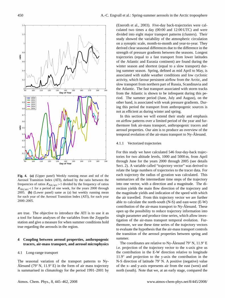
Fig. 4. (a) (Upper panel) Weekly running mean and std of theAerosol Transition Index (ATI), defined by the ratio between thefrequencies of ratiosRAit/acc>1 divided by the frequency of ratiosRAit/acc<1 for a period of one week, for the years 2000 through2005. (b) (Lower panel) same as (a) but weekly running meanfor each year of the Aerosol Transition Index (ATI), for each year2000–2005.

are true. The objective to introduce the ATI is to use it asa tool for future analyses of the variables from the Zeppelinstation and give a measure for when summer conditions holdtrue regarding the aerosols in the region.

4 Coupling between aerosol properties, anthropogenictracers, air-mass transport, and aerosol microphysics

4.1 Long-range transport

The seasonal variation of the transport patterns to Ny-Alesund (79◦ N, 11.9◦ E) in the form of air mass trajectoryis summarised in climatology for the period 1991–2001 by

(Eneroth et al., 2003). Five-day back-trajectories were cal-culated two times a day (00:00 and 12:00 UTC) and weredivided into eight major transport patterns (clusters). Theirstudy showed the variability of the atmospheric circulationon a synoptic scale, month-to-month and year-to-year. Theyderived clear seasonal differences due to the difference in thestrength of pressure gradients between the seasons. Longesttrajectories (equal to a fast transport from lower latitudesof the Atlantic and Eurasia continent) are found during thewinter season and shortest (equal to a slow transport) dur-ing summer season. Spring, defined as mid April to May, isassociated with stable weather conditions and low cyclonicactivity, which favour persistent airflow from the Arctic, andslow transport from northern part of Russia, Scandinavia andthe Atlantic. The fast transport associated with storm tracksfrom the Atlantic is shown to be infrequent during this pe-riod. The summer period (June, July and August), on theother hand, is associated with weak pressure gradients. Dur-ing this period the transport from anthropogenic sources isnot as efficient as during winter and spring.

In this section we will extend their study and emphasison airflow patterns over a limited period of the year and fur-thermore link air-mass transport, anthropogenic tracers andaerosol properties. Our aim is to produce an overview of thetemporal evolution of the air-mass transport to Ny-Alesund.

4.1.1 Vectorized trajectories

For this study we have calculated 546 four-day-back trajec-tories for two altitude levels, 1000 and 5000 m, from Aprilthrough June for the years 2000 through 2005 (see detailsSect. 2). A variable called “trajectory vector” was derived torelate the large numbers of trajectories to the tracer data. Foreach trajectory the radius of gyration was calculated. Thissummarizes all the intermediate time steps of the trajectoryinto one vector, with a direction and a magnitude. The di-rection yields the main flow direction of the trajectory andthe magnitude yields and indication of the speed with whichthe air travelled. From this trajectory vector we are furtherable to calculate the north-south (N-S) and east-west (E-W)contribution of the air-mass transport to Ny-Alesund. Theseopen up the possibility to reduce trajectory information intosingle parameter and produce time series, which allow inves-tigation of the air-mass transport temporal evolution. Fur-thermore, we use these time series of the trajectory vectorsto evaluate the hypothesis that the air-mass transport controlsthe transition of the aerosol properties between spring andsummer.

The coordinates are relative to Ny-Alesund 79◦ N, 11.9◦ Ei.e. projection of the trajectory vector to the x-axis give usthe contribution in the E-W direction relative to longitude11.9◦ and projection to the y-axis the contribution in theN-S direction of latitude 79◦ N. A positive (negative) valueof the x- and y-axis represents air from the east (west) andnorth (south). Note that we, at an early stage, compared the



100 120 140 160 180−1

−0.5

0

0.5

1North

South

(a)

100 120 140 160 180−1

−0.5

0

0.5

1(b)

100 120 140 160 180−1

−0.5

0

0.5

1North

South

(c)

100 120 140 160 180−1

−0.5

0

0.5

1(d)

100 120 140 160 180−1

−0.5

0

0.5

1

Day of Year

North

South

(e)

100 120 140 160 180−1

−0.5

0

0.5

1

Day of Year

(f)

Fig. 5. The vectorized trajectories arriving to altitude-level 1000 m plotted with time (day of the year) for each year 2000–2005(a–f). Y-axisshows the normalized North-South (N-S) contribution for the air-mass transport.

four-day-back trajectories with ten-day-back trajectories andthey did not show significant difference with respect to ourapproach to the air mass origin used in the study. Thereforewe continue to use four-day trajectories throughout the study.

4.1.2 Transport patterns

Combining the N-S and E-W component for each day givesus the horizontal information of the trajectory with respect tothe direction and magnitude. Figure 5a–f presents the calcu-lated N-S contribution for each day that the trajectory arrivedto level 1000 m (BL) for the time period from 2000 through2005 (similar research has been performed for level 5000 m(FT), as it does not give any additional information it is notshown here). From Figs. 5a–f there are no apparent trendsthat could link to and explain the transition in aerosol prop-erties, i.e. corresponding rapid and repeating change from amore polluted origin in the spring to a more clean origin inthe summer.

The short analysis above has essentially provided informa-tion about the horizontal transport. To investigate the verti-cal dimension we also calculated the time the trajectory has

spent in the boundary layer during the last four days of itstransport to Ny-Alesund. The different years are then av-eraged for each day of the investigated time period and areexpressed as fraction time to the total time-length of the tra-jectory. In this context we define the BL to be altitudes below2000 m. This altitude often represents the top of the low-level clouds as seen by MPL at Ny-Alesund. The exceptionsare cases when the air arrives within a sector that belongsto the Arctic basin i.e. representing the area within the twotangents with origins in the coordinates of Ny-Alesund andtangents the north coast of Greenland and the northern coastof Siberia. Within this sector the BL height is defined as1000 m. This difference in definition in BL takes into ac-count the stable stratification over the pack ice, especiallyduring the summer months (Nilsson, 1996).

The calculated fraction ranges from 0 to 1, where 1 rep-resents a trajectory that spends all its time in the BL. Thetemporal evolution of this fraction is depicted in Fig. 6. Theupper and lower panels represent trajectories arriving to Ny-Alesund at the altitude level 1000 and 5000 m, respective.Not surprisingly trajectories arriving at a lower altitude spend



90 100 110 120 130 140 150 160 170 1800.3

0.4

0.5

0.6

0.7

0.8

frac

tion

Arriving altitude 1000m

90 100 110 120 130 140 150 160 170 1800

0.02

0.04

0.06

0.08

0.1

0.12

0.14

Day of Year

frac

tion

Arriving altitude 5000m

Fig. 6. The relative fraction mean time, each day trajectory hasspent in the boundary layer (BL) defined as altitudes below 2000 m(1000 m for the Arctic region), for the years 2000–2005. The upperpanel represents trajectory that arrive to the altitude level of 1000 mand lower panel trajectories that arrive to the altitude of 5000 m.

more time in the BL. Comparing the start and end of the pe-riod we notice a decreasing trend in ratio of high-level tra-jectories spending time in the BL (lower panel). But thesetrends are not very strong and do not show the radical changebetween day 140 and 150 that the aerosol properties do.

4.2 Anthropogenic tracers

In previous sections we have shown that transport alonecannot explain the transition in aerosol properties observedon annual basis. Here we will explore the possibility thatthe combination of various transport patterns and seasonalchanges in the anthropogenic sources strength can shed alight on observed aerosol microphysics. The tracers used inthis analysis serve as proxy for air-mass characteristics. Theyare not necessarily intended to address long-range transportof small aerosol particles, but rather to indicate changes inthe composition of the air with respect to aerosol precursorsand pre-existing particles. To follow this hypothesis we usedata of anthropogenic tracers SO2, CO and210Pb observed atthe Zeppelin station and focused on their temporal variation.

SO2 is one of the major anthropogenic trace gases andhighly relevant to aerosol properties. Additional to the an-thropogenic source it also has a natural biogenic sourcecontributing to SO2 in the atmosphere through oxidationof dimethyl sulphide (DMS) (Li and Barrie, 1993; Li etal., 1993; Ferek et al., 1995). We also explored measure-ments of CO and210Pb because in the Arctic the occur-rence of these can be attributed exclusively to sources out-side of the Arctic. We will use them as major tracers foranthropogenic source regions (Paatero et al., 2003). Fig-ure 7a and b shows the weekly running mean of SO2 and

90 100 110 120 130 140 150 160 170 180 1900

0.1

0.2

0.3

0.4

0.5

0.6

0.7

Day of Year

SO

2 (ug

Sm

−3)

a

90 100 110 120 130 140 150 160 170 180 19060

80

100

120

140

160

180

200

b

Day of Year

CO

(pp

b(v)

)

Fig. 7. Weekly running mean (thick lines) and plus minus one stan-dard deviation (thin lines) of the trace gases SO2 (a) and CO(b)measured at the Zeppelin station for the years 2000–2005 and 2002–2004, respectively.

CO. SO2 shows a large intra-annual variability in data forthe period with episodes of high values in April and May andrather low concentration in June. The concentrations rangebetween a minimum value of 0.01µgS m−3 (effective detec-tion limit) to a 2.13µgS m−3 and a median of 0.07µgS m−3.The monthly mean and standard deviation of SO2 show themaximum to occur in May with 0.14(0.28)µgS m−3 and atrend that decreases towards June with corresponding valuesof 0.07(0.04)µgS m−3 (cf. Table 2).

The high variability of SO2 in April and May reflects thefrequent fast transport from anthropogenic sources that takeplace during springtime, whereas in June it is more asso-ciated with lower background concentrations perturbed byoccasional higher values but not as high as April and May.The source of DMS is anticipated to be at its largest in latesummer (August) according to study by (Ferek et al., 1995).They reported Arctic DMS concentration up to 300 ppt,



while background concentrations stayed at a few tens ofppt. If the observed DMS concentrations were convertedto sulfur (S) at 100% efficiency it would give a backgroundlevel of approximately 0.04µgS m−3 and the highest peakwould correspond to about 0.4µgS m−3. This maximumvalue is still well below the peaks observed in the springtimeat the Zeppelin station. There is nothing in the SO2 trendthat would suggest that an increased biogenic source wouldexplain the observed sudden transition in aerosol proper-ties. For year 2005, SO2 shows a mean concentration of0.13µgS m−3, which differs from other years where themean concentration is much lower (0.07µgS m−3). Over allsample years we note that after day 140 SO2 infrequently ex-ceeds 0.07µgS m−3. The only characteristic that could relateto the aerosol transition is the fewer occurrences of higherSO2 levels after day 140. However, this trend would tend todecrease the potential for new particle formation.

CO in Fig. 7b follows a clear decreasing trend duringthe period. Carbon monoxide has a longer residence time(around 90 days) in the atmosphere compared to SO2 (5–7 days), which explains much of different features betweenFig. 7a and b. The total mean and standard deviation of COconcentration is 135(25) ppbv, which is about 9% lower com-pared to yearly base mean presented by Beine (1999). Asidefrom some small deviation around day 155, the trend in COshows a rather smooth decrease over time. Variability is alsorelatively constant over the period. As OH acts as a majorsink for CO, the annual cycle of hydroxyl radical (•OH) isof major importance for the seasonal evolution of CO. OH isproduced by photochemical reactions and therefore dependson incoming solar radiation. Observations show that CO ac-cumulates in the Arctic troposphere during wintertime dueto transport processes and the fact that sink processes by OHare not available. During spring when the sun rises the sinkprocesses for CO become active and the CO concentrationsstart to decrease, with the minimum reached in summer (Di-anovklokov and Yurganov, 1989). The steady state decreaseof CO mixing ratios, only slightly perturbed by local maxi-mum, correlated with episodes of higher SO2, also indicatesthat dilution and mixing with clean air masses and photo-chemical sink of CO dominates over the source in the formof long-range transport during April-June period.

Lead-210 (210Pb) originates almost exclusively from con-tinents and as such it is a tracer of air masses having ratherrecent contact with landmasses. With its long lifetime (half-life 22 years) the atmospheric lifetime is mainly governedby the lifetime of the aerosols (Paatero et al., 2003). Mostof the atmospheric210Pb is attached to accumulation-modeaerosols. Based on the activity ratio of210Pb and its progeny;mean aerosol residence times can be estimated. In the presentstudy we only investigate the temporal variation of210Pbdata itself. The annual variation of the activity concentra-tion of 210Pb at the Zeppelin station was between 11 and620µBq m−3 for the year 2001 (Paatero et al., 2003). Themaximum was observed in March-April and the minimum in

90 100 110 120 130 140 150 160 170 1800

50

100

150

200

250

300

350

400

Day of Year

210 P

b (

µBqm

−3)

90 100 110 120 130 140 150 160 170 180 1900

50

100

150

200

250

210 P

b uB

q m

−3

90 100 110 120 130 140 150 160 170 180 1904

6

8

10

12

14

16

18

Day of Year

cm−2

Lead−210 average

Accu. Surface

Fig. 8. (a) (Upper panel) the activity concentration of lead-210 onaerosols measured at the Zeppelin station 2001–2005. Weekly run-ning average and error bars representing one standard deviation.(b)(Lower panel) the averaged lead-210 concentration plotted togetherwith the average accumulation-mode (90–630 nm) particles surface.

summer. In the present study the210Pb activity concentra-tion vary between 0 and 552µBq m−3. The data presentedin Fig. 8a agree well with the single-year study by Paatero etal. (2003); maximum values in April with a monthly meanand standard deviation of 165 and 134µBq m−3, respec-tively, and a much lower mean in June of 35(27)µBq m−3.

Lead-210 is one of the tracers investigated in this studythat shows a notable change in both the rate at which it de-creases and its variability. In particular the decrease in vari-ability is very evident. It is worthy to note again that210Pb isassociated with accumulation-mode particles and thus couldbe a proxy of relative increase or decrease of the aerosol sur-face area, which are also dominated by accumulation-modeaerosol (Fig. 8b).



100 110 120 130 140 150 160 170 180−1

−0.5

0

0.5

1

North

South

100 110 120 130 140 150 160 170 1800

100

200

300

400

500

600

cm−3

100 110 120 130 140 150 160 170 180−1

−0.5

0

0.5

1

East

West

April May June

100 110 120 130 140 150 160 170 1800

100

200

300

400

500

600

cm−3

Day of Year

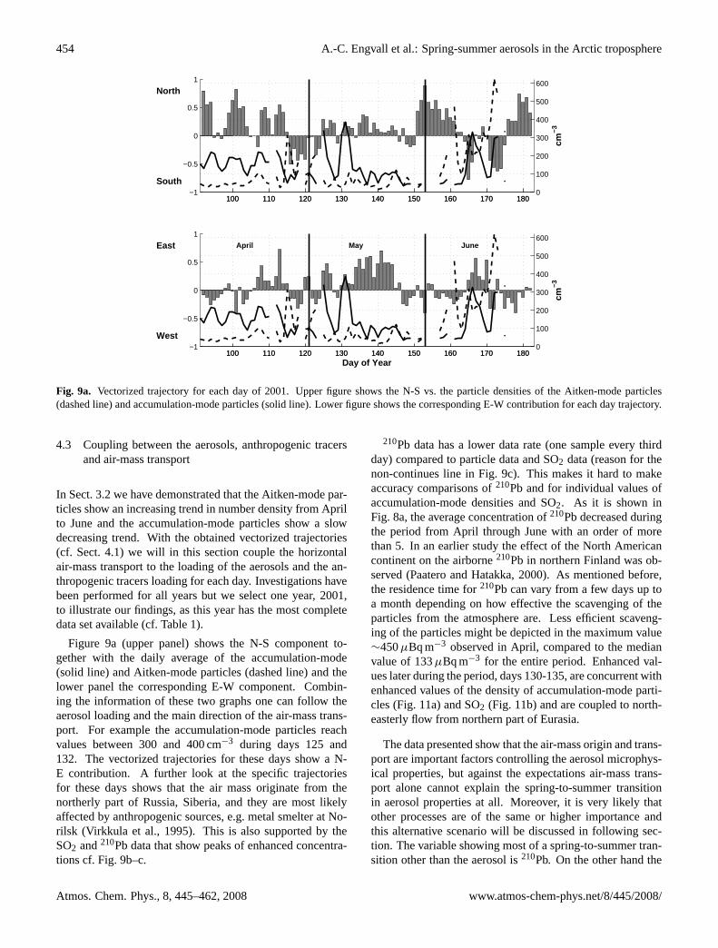
Fig. 9a. Vectorized trajectory for each day of 2001. Upper figure shows the N-S vs. the particle densities of the Aitken-mode particles(dashed line) and accumulation-mode particles (solid line). Lower figure shows the corresponding E-W contribution for each day trajectory.

4.3 Coupling between the aerosols, anthropogenic tracersand air-mass transport

In Sect. 3.2 we have demonstrated that the Aitken-mode par-ticles show an increasing trend in number density from Aprilto June and the accumulation-mode particles show a slowdecreasing trend. With the obtained vectorized trajectories(cf. Sect. 4.1) we will in this section couple the horizontalair-mass transport to the loading of the aerosols and the an-thropogenic tracers loading for each day. Investigations havebeen performed for all years but we select one year, 2001,to illustrate our findings, as this year has the most completedata set available (cf. Table 1).

Figure 9a (upper panel) shows the N-S component to-gether with the daily average of the accumulation-mode(solid line) and Aitken-mode particles (dashed line) and thelower panel the corresponding E-W component. Combin-ing the information of these two graphs one can follow theaerosol loading and the main direction of the air-mass trans-port. For example the accumulation-mode particles reachvalues between 300 and 400 cm−3 during days 125 and132. The vectorized trajectories for these days show a N-E contribution. A further look at the specific trajectoriesfor these days shows that the air mass originate from thenortherly part of Russia, Siberia, and they are most likelyaffected by anthropogenic sources, e.g. metal smelter at No-rilsk (Virkkula et al., 1995). This is also supported by theSO2 and210Pb data that show peaks of enhanced concentra-tions cf. Fig. 9b–c.

210Pb data has a lower data rate (one sample every thirdday) compared to particle data and SO2 data (reason for thenon-continues line in Fig. 9c). This makes it hard to makeaccuracy comparisons of210Pb and for individual values ofaccumulation-mode densities and SO2. As it is shown inFig. 8a, the average concentration of210Pb decreased duringthe period from April through June with an order of morethan 5. In an earlier study the effect of the North Americancontinent on the airborne210Pb in northern Finland was ob-served (Paatero and Hatakka, 2000). As mentioned before,the residence time for210Pb can vary from a few days up toa month depending on how effective the scavenging of theparticles from the atmosphere are. Less efficient scaveng-ing of the particles might be depicted in the maximum value∼450µBq m−3 observed in April, compared to the medianvalue of 133µBq m−3 for the entire period. Enhanced val-ues later during the period, days 130-135, are concurrent withenhanced values of the density of accumulation-mode parti-cles (Fig. 11a) and SO2 (Fig. 11b) and are coupled to north-easterly flow from northern part of Eurasia.

The data presented show that the air-mass origin and trans-port are important factors controlling the aerosol microphys-ical properties, but against the expectations air-mass trans-port alone cannot explain the spring-to-summer transitionin aerosol properties at all. Moreover, it is very likely thatother processes are of the same or higher importance andthis alternative scenario will be discussed in following sec-tion. The variable showing most of a spring-to-summer tran-sition other than the aerosol is210Pb. On the other hand the



100 110 120 130 140 150 160 170 180−1

−0.5

0

0.5

1

North

South

100 110 120 130 140 150 160 170 1800

0.5

1

1.5

2

ugS

m−3

100 110 120 130 140 150 160 170 180−1

−0.5

0

0.5

1

East

West

April May June

100 110 120 130 140 150 160 170 1800

0.5

1

1.5

2

ugS

m−3

Day of Year

Fig. 9b. Each day vectorized trajectory for 2001. Upper figure shows the N-S together with SO2 concentration (line). Lower figure showsthe corresponding E-W contribution for each day trajectory.

90 100 110 120 130 140 150 160 170 180−1

−0.5

0

0.5

1

North

South

90 100 110 120 130 140 150 160 170 1800

100

200

300

400

uBqm

−3

90 100 110 120 130 140 150 160 170 180−1

−0.5

0

0.5

1

East

West April May June

90 100 110 120 130 140 150 160 170 1800

100

200

300

400

uBqm

−3

Day of Year

Fig. 9c. Each day vectorized trajectory for 2001. Upper figure shows the N-S together with210Pb concentration (stars). Lower figure showsthe corresponding E-W contribution for each day trajectory.

lifetime of 210Pb in the atmosphere is intimately linked toaerosols through being attached to accumulation-mode parti-cles (cf. Fig. 8b). The accumulation-mode particles are typ-ically where the largest surface area can be found and thusthe largest sink for condensable species. New particle for-mation is a non-linear process that involves the competitionbetween the sink of condensable species and the source ofthe same. Therefore, the alternative scenario can be formu-

lated: Can annual systematic changes in the source strengthand sink rate of the condensable species together give thetype of transition that the aerosol properties show?



90 100 110 120 130 140 150 160 170 1800

2

4

6

8

10

12x 10

7

Day of Year

Equ

libriu

m c

oncn

etra

tion

H2S

O4 (

mol

ecul

es c

m−3

)

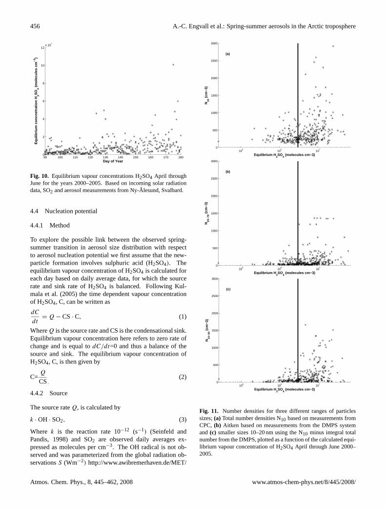
Fig. 10. Equilibrium vapour concentrations H2SO4 April throughJune for the years 2000–2005. Based on incoming solar radiationdata, SO2 and aerosol measurements from Ny-Alesund, Svalbard.

4.4 Nucleation potential

4.4.1 Method

To explore the possible link between the observed spring-summer transition in aerosol size distribution with respectto aerosol nucleation potential we first assume that the new-particle formation involves sulphuric acid (H2SO4). Theequilibrium vapour concentration of H2SO4 is calculated foreach day based on daily average data, for which the sourcerate and sink rate of H2SO4 is balanced. Following Kul-mala et al. (2005) the time dependent vapour concentrationof H2SO4, C, can be written as

dC

dt= Q − CS· C, (1)

WhereQ is the source rate and CS is the condensational sink.Equilibrium vapour concentration here refers to zero rate ofchange and is equal todC/dt=0 and thus a balance of thesource and sink. The equilibrium vapour concentration ofH2SO4, C, is then given by

C=Q

CS.(2)

4.4.2 Source

The source rateQ, is calculated by

k · OH · SO2, (3)

Where k is the reaction rate 10−12 (s−1) (Seinfeld andPandis, 1998) and SO2 are observed daily averages ex-pressed as molecules per cm−3. The OH radical is not ob-served and was parameterized from the global radiation ob-servationsS (Wm−2) http://www.awibremerhaven.de/MET/

105

106

107

0

500

1000

1500

2000

2500

3000

Equlibrium H2SO

4 (molecules cm−3)

N10

(cm

−3)

(a)

105

106

107

0

500

1000

1500

2000

2500

3000

Equlibrium H2SO


N20

−79 (

cm−3

)

(b)

105

106

107

0

500

1000

1500

2000

2500

3000

Equlibrium H2SO


N10

−20 (

cm−3

)

(c)

Fig. 11. Number densities for three different ranges of particlessizes;(a) Total number densities N10 based on measurements fromCPC,(b) Aitken based on measurements from the DMPS systemand(c) smaller sizes 10–20 nm using the N10 minus integral totalnumber from the DMPS, plotted as a function of the calculated equi-librium vapour concentration of H2SO4 April through June 2000–2005.


http://www.awibremerhaven.de/MET/NyAlesund/fulltimeresquery.html


NyAlesund/fulltimeresquery.html). To calculate OH concen-tration, S was simply scaled by a maximum value (387) ofthe total data set for observed diffuse solar radiation and mul-tiplied by 5×106 according to Eq. (4).

S · 5 × 106

387. (4)

As actual•OH concentrations are unknown to us, this scal-ing is entirely arbitrary and only serves to reproduce typicalvalues for•OH concentrations frequently reported in the lit-erature (Seinfeld and Pandis, 1998).

4.4.3 Sink

The condensational sink is calculated based on observed sizedistributions following Kulmala et al. (2001), including thecorrection factor for the transition between the molecular andcontinuum regimes given by:

CS=2πD

∞∫

0

dpβM(dp)n(dp)ddp=2πD∑

i

βMdp,iNi (5)

WhereD is the diffusion coefficient,n(dp) is the particlesize distribution function andNi is the concentration of par-ticles in the size sectioni. For the transitional correction fac-tor for the mass fluxβM we use the Fuchs-Sutugin expression(Fuchs and Sutugin, 1971).

To derive the condensational sink, CS (s−1), the hourlyaveraged size-distributions for particles larger than 90 nm(accumulation-mode particles) were used. The reason for re-stricting the condensational sink only to the accumulation-mode particles is that Aitken particles are a result of rela-tively recent particle production, whereas the accumulation-mode particles were most likely already present and availableas a sink at the time the new particles were formed. CS wascalculated from the hourly average of particle data. We ex-clude days with less than 10 data points (hourly averages).It should also be noted that CS is calculated based on dryaerosol due to the measurement set-up (cf. Sect. 2.2).

Typically, the Arctic summer boundary layer is often veryhumid. We have evaluated the relative humidity (RH) datafrom the Zeppelin station to investigate the hygroscopic ef-fect on aerosols and CS. The influence of RH will affect thecalculated condensation sink that is used to estimate the equi-librium concentration of sulphuric acid. The relevant issuehere is if including RH makes CS change with time differ-ently than by not including RH.

RH data are available only for years 2002 to 2005 andhence not for the entire data set. We consider hygroscopicgrowth for an H2SO4-aerosol, following the approximationby Kopke et al. (1997). The result shows that the hygro-scopic growth affects the aerosol with almost the same mag-nitude over the entire period. Comparing CS for these twoconditions, with or without including hygroscopic growth,show a CS increase with a factor 1.8 in April, 1.7 in May

and a factor of 2 in June. Hence the equilibrium concen-tration of H2SO4 vapour will decrease about a factor of twoover the entire 3-month period, but the difference betweenthe months are not large enough to explain the transition ob-served in equilibrium concentration of H2SO4. If anything,the slightly higher CS in summer compared to spring wouldtend to make the transition less pronounced. We thereforeuse the dry aerosol size, which makes it possible for us touse a larger data set.

4.4.4 Result

Following the above formulas the equilibrium H2SO4 con-centration was calculated based on the average incoming ra-diation, SO2 and CS for each day. In Fig. 10 these valuesfor the data set is plotted as function of day. The data rangesfrom close to zero to around 1×108 molecules cm−3with anincreasing trend with time, even though the main part of datafalls between 8×105 and 3×107 molecules cm−3. We wereinterested to find out whether there is any particular value ofC above where small particles are more likely to occur. To dothis we analysed the observed integral aerosol number densi-ties of various sizes versus C Fig. 11a–c. There are differentamounts of data in each scatter plot presented in Fig. 11a–cdue to reduction of the time resolution for individual instru-ments. Note that data in Fig. 11a and b are entirely indepen-dent, whereas in Fig. 11c the accumulation mode part of thesize distribution enters both variables.

All three scatter plots present a systematic trend with morefrequent high number densities as C increases. However,it is difficult to distinguish a very clear critical value for Cthat would indicate a nucleation threshold. Based on thethree scatter plots it appears that a value of C above approxi-mately 3×106 molecules cm−3 separates C values with gen-erally low number densities and C values associated with thehighest number densities.

Note that we work with daily averages given by measureddata from Ny-Alesund. Newly formed particles may takeseveral hours, up to a day, to reach a size of 10 nm (detectablesize for the instrument) due to the low concentration of con-densable material in the Arctic. Hence, the observed condi-tions when there are high number-densities of aerosols in Ny-Alesund are not necessarily identical to the conditions exist-ing where the particle formation actually took place. To givethe reader a feeling for the spatial scale of our approach wemight think of how far an air parcel is transported in one day.Given a mean wind speed of 5 ms−1 this distance is equiv-alent to more than 400 km transport during one day. Thismeans that processes taking place 400 km from Ny-Alesundaffect our daily averages.

The present study is not aimed at a detailed analysis ofthe nucleation process, but rather to characterize the condi-tions related to the observed changes in aerosol characteris-tics. By necessity the analysis of the data becomes schematicin many aspects, as there are many processes that interplay.


http://www.awibremerhaven.de/MET/NyAlesund/fulltimeresquery.html


90 100 110 120 130 140 150 160 170 1800

0.1

0.2

0.3

0.4

0.5

0.6

0.7

0.8

0.9

Day of Year

Rat

io

(a)0.6E70.9E71.1E7

90 100 110 120 130 140 150 160 170 1800

0.1

0.2

0.3

0.4

0.5

0.6

0.7

0.8

0.9

Day of Year

Rat

io

(b)0.6E70.9E71.1E7

Fig. 12. (a) Fraction for when a certain criteria,0.6×107 molecules cm−3(solid) 0.9×107 molecules cm−3

(dashed) and 1.1×107 molecules cm−3 (dotted) of the equi-librium vapour concentrations of H2SO4 occur.(b) Same as (a) butexcluded for polluted events.

We are interested in singling out the most important factorsand therefore we omit details in favour of trends. The resultshere will therefore only illustrate the trend in data found inthe Arctic region and will not describe the nucleation pro-cesses in detail.

4.4.5 Trace gases influence on observed aerosol loading

Whether or not the critical value is below or above3×106 molecules cm−3 we can see the potential effect ofsuch a threshold on the size distribution over time. We maythink of it as a nucleation potential. Moreover, it is not onlyof interest if the conditions meet the threshold, but also towhat extent C may exceed above this values, as seen fromFig. 11a. We illustrate this by making a weekly moving av-erage of the ratio between the number of data points exceed-ing a certain threshold, divided by the total number of datapoints for the time window over all six years. If the equilib-

rium threshold is reached often we expect that formation ofparticles occur readily during that time. The higher the valueof this threshold, the more vigorous we expect the particleformation to be.

We explore three different values of the H2SO4 equi-librium concentration threshold: 0.6×107; 0.9×107; and1.1×107 molecules cm−3 (see Fig. 12a). From comparingthe different ratios it is clear that changing the threshold from0.6×107 to 1.1×107 molecules cm−3 has the largest impacton the evolution of the ratios in the middle of the time pe-riod, where the reduction in the ratio is twice as large as atboth ends of the time period. Thus, the difference betweenthe ratios in April and May compared with June are accen-tuated. This is most evident for the highest threshold value;there the ratio increases from low values to about 0.2 overthe first two months and then quickly increases to above 0.4in about a week’s time.

A small amount of data (about 6%) is clearly affected byrapid transport from anthropogenic sources evident in thevery high SO2 concentrations for the time period. These highSO2 concentrations would yield enhanced values of equilib-rium H2SO4. As we only consider the aerosol size distri-bution up to 630 nm (due to the limitation of the measur-ing equipment) in calculating CS, it is possible that a sig-nificant contribution to CS from larger particles is missedduring strong pollution events. This would result in an un-derestimation of C, whereas nucleation events are typicallyquenched in polluted air due to large aerosol surface area.To test the influence of these events on our results we re-peated the ratio calculation after screening data where SO2exceed 0.6×107 molecules per cm−3 (see Fig. 12b). Thislimit was chosen by investigating data for when SO2 con-centration reached high values that were probably influencedby anthropogenic sources. Excluding the pollution eventsgenerates no large changes between Fig. 12a and b. But ex-cluding these outliers makes the transition from low ratios inthe beginning of the period to higher ratios in June somewhatclearer. The highest threshold for instance never occurs be-fore day 115. Between day 115 and day 145 the fraction oftime the threshold is exceeded increase to 20%. Only 10 dayslater this fraction is more than doubled and from about day155 the fraction hovers around 50%. Hence in late May andbeginning of June the occurrence of the potential conditionsfor particle formation increases dramatically.

5 Discussion

Transport patterns and source strengths of anthropogenictracers change over the year with the net effect that the Arc-tic atmosphere in the late winter and spring period is themost polluted and that summer is the cleanest period ofthe year. Over the time period from spring to summer, theaerosol characteristics change from being dominated by theaccumulation-mode to being primarily of the Aitken-mode



variety. Our observations and analysis show that this transi-tion is not typically a gradual change but occur over a rathershort period in late May/early June each year, and takesaround 10 days. Intrigued by the temporal persistence ofthe transition we systematically investigated pertinent trac-ers and transport patterns over the period April–June duringa six-year period (2000–2005).

If the transition from spring- to summer-aerosol could beexplained by transport alone, we would expect that the maintransport pattern should change from one regime to anotheri.e. a change from anthropogenic sources at lower latitudesto biogenic sources from the north, which in present study isnot the case. Although seasonal changes in the flow patternexist (Eneroth et al., 2003; Stohl, 2006) our analysis couldnot reveal any systematic pattern that could help explain therapid transition observed for the aerosol properties.

The levels of DMS may be largest in the latter part of thesummer (Ferek et al., 1995), but the overall concentrationsof SO2 decrease over the investigated time period. Thereforethere may be a debate about what process actually formed theSO2 molecule; anthropogenic versus natural, and a biogenicsource, via its sulphur cycle, cannot explain the transition.The fact that the SO2 values are at their lowest during theperiod with most active particle production is perhaps unex-pected. Shaw (1989) discussed particle formation in cleanareas and suggested that one viable pathway is the cleaningof pre-existing aerosol area through precipitating clouds.

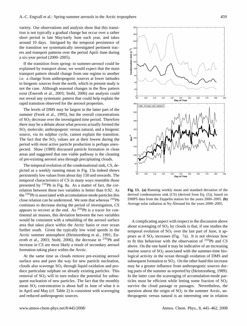
The temporal evolution of the condensational sink, CS, de-picted as a weekly running mean in Fig. 13a indeed showspersistently low values from about day 150 and onwards. Thetemporal characteristics of CS in many ways resemble thosepresented by210Pb in Fig. 8a. As a matter of fact, the cor-relation between these two variables is better than 0.92. Asthe210Pb is associated with accumulation-mode particles thisclose relation can be understood. We note that whereas210Pbcontinues to decrease during the period of investigation, CSappears to recover at the end. As210Pb is a tracer for con-tinental air masses, this deviation between the two variableswould be consistent with a rebuilding of the aerosol surfacearea that takes place within the Arctic basin or over oceanfurther south. Given the typically low wind speeds in theArctic summer atmosphere (Heintzenberg et al., 1991; En-eroth et al., 2003; Stohl, 2006), the decrease in210Pb andincrease in CS are most likely a result of secondary aerosolformation taking place within the Arctic.

At the same time as clouds remove pre-existing aerosolsurface area and pave the way for new particle nucleation,clouds also scavenge SO2 through liquid oxidation and pro-duce particulate sulphate on already existing particles. Thisremoval of SO2 will in turn reduce the potential for subse-quent nucleation of new particles. The fact that the monthlymean SO2 concentration is about half in June of what it isin April and May (cf. Table 2) is consistent with scavengingand reduced anthropogenic sources.

90 100 110 120 130 140 150 160 170 180 1900

20

40

60

80

100

120

140

160

180

200

Day of Year

Con

dens

atio

n si

nk (

s−1

)

90 100 110 120 130 140 150 160 170 180 1900

50

100

150

200

250

300

350

400

Day of Year

Wm

−2

Average solar radiation

Fig. 13. (a)Running weekly mean and standard deviation of thederived condensations sink (CS) (derived from Eq. (5)), based onDMPS data from the Zeppelin station for the years 2000–2005.(b)Average solar radiation at Ny-Alesund for the years 2000–2005.

A complicating aspect with respect to the discussion aboveabout scavenging of SO2 by clouds is that, if one studies thetemporal evolution of SO2 over the last part of June, it ap-pears as if SO2 increases (Fig. 7a). It is not obvious howto fit this behaviour with the observation of210Pb and CSabove. On the one hand it may be indicative of an increasingmarine source of SO2 associated with the summer-time bio-logical activity in the ocean through oxidation of DMS andsubsequent formation to SO2. On the other hand this increasemay be a greater influence from anthropogenic sources dur-ing parts of the summer as reported by (Heintzenberg, 1989).In the latter case the scavenging of accumulation-mode par-ticles must be efficient while letting some fraction of SO2survive the cloud passage or passages. Nevertheless, thequestion about the origin of SO2 in the summer Arctic, an-thropogenic versus natural is an interesting one in relation



to aerosol-cloud interactions and climate forcing, and needsfurther investigation.

The third leg in this simple method to determine the nu-cleation potential is solar radiation, which in turn is a proxyfor OH in the atmosphere. A close relationship betweenthe yearly cycle of particle number density and incomingsolar radiation at Ny-Alesund, which supports the impor-tance of photochemical reactions has been shown by Stromet al. (2003). At about mid-March the sun returns to the Sval-bard region and the summer solstice occur about three weeksinto June. Hence, the spring-to-summer period presents adramatic increase in the amount of radiation that reaches Ny-Alesund. Therefore, the decrease in the precursor gas SO2due to changes in transport patterns is more than compen-sated for by the combined effect of an increased radiationflux and decreased condensational sink.

This is illustrated by using some simple numbers. SO2decrease by about a factor of 2 between the beginning andend of the time period (cf. Table 2). The condensationalsink decreases over the same time by about a factor of 2(cf. Fig. 13a). However, the weekly median radiation in-creases by about a factor of 5 (Fig. 13b). Hence, the tempo-ral evolution of CS and SO2 largely compensate each otherand the nucleation potential is mainly driven by the radia-tion. The net effect is that the nucleation potential reachessome critical value at about the same time each year.

Particle nucleation is highly non-linear and some criticalsuper-saturation of condensable vapour must be reached be-fore new particles will form. Below this value nucleationdoes not readily occur. For instance, the more this criticalvalue is exceeded, the larger the chance is that the newlyformed particles will grow to sizes that can be detected bythe instruments at the Zeppelin station. Based on the tempo-ral evolution of the Aitken mode in Fig. 3a and the aerosoltransition index in Fig. 4a and b we believe that this criticalvalue is typically meet every year around day 145 plus or mi-nus a week. Hence we believe that photochemical reactionsgovern much of the aerosol dynamics in the Arctic.

The whole picture is further complicated by the fact thatremote sensing data shows similar sudden change in aerosolproperties, which indicates the whole troposphere to be in-volved in a similar transition. Remote sensing within theStratospheric Aerosol and Gas Experiment (SAGE) II and IIIsuggests a change between spring and summer for the opticalproperties of the Arctic aerosol in the upper free troposphereabove 4 km altitude (Treffeisen et al., 2006). Whether sameprocesses in the BL control this remains to be investigated.

6 Summary and conclusions

The main motivation for this study was to investigate thespring – summer period (April, May, and June), with em-phasis on the transition in aerosol properties observed in theArctic troposphere on an annual basis. In the study we have

used four-day-back trajectories and long-term observationsof aerosols and trace gases from the Zeppelin station, Sval-bard. We have described the difference between the peri-ods of spring and summer, the transition between them, andwe have attempted to link the observations to the large-scalecirculation and influences from natural and anthropogenicsources of aerosols and gases. We have investigated the hy-pothesis that air-mass transport to the Arctic controls the sys-tematic change in the physical properties of aerosols (i.e.from being dominated by accumulation-mode in spring tobeing Aitken-mode dominated in summer) that are observedat the Zeppelin station. To summarise this work, we endedup with four main conclusions:

1. Using air mass back-trajectories we have shown thattransport alone cannot explain the repeating rapid tran-sition from spring-type to summer-type aerosol ob-served in the Arctic troposphere.

2. Blocking the advection of the polluted air masses fromsouth into the Arctic is important contributor to trans-port, but it should be seen more as a necessary prerequi-site rather than the main process controlling the spring-summer transition in aerosol properties. The reductionof the anthropogenic contribution (using CO as tracer)during the investigated period presents a rather smoothtrend and cannot alone explain the sudden change inaerosol properties.

3. With a simplified model, which delivers the nucleationpotential for new-particle formation in the form of equi-librium vapour concentration of H2SO4, we suggest thatthe aerosol microphysical properties are the result ofa delicate balance between incoming solar radiation,transport, and condensational sink processes.

4. The temporal evolution of the condensational sink andSO2 concentrations indicate that, to a large degree, theycompensate each other and the nucleation potential ismainly driven by solar radiation. The strong seasonalityof the solar angle in the Arctic results in the nucleationpotential reaching some critical value about the sametime each year. This is consistent with a repeating pat-tern of aerosol transition between spring and summer.

At this time, it is not clear how and to what extent pro-cesses in the boundary layer and the free troposphere areinterlinked. In order to get better insight into this phe-nomenon, airborne in-situ measurements covering the wholetropospheric column are necessary.

Acknowledgements. The authors wish to acknowledge C. Lunder(NILU), B. Noone (ITM) and J. Waher (ITM) for providing us withdata from the Zeppelin station. The monitoring at the Zeppelin sta-tion is supported by the Swedish Environmental Protection Agencyand by the Swedish National Science Foundation. Support has alsobeen received from the Swedish Polar Secretariat. The FMI’s210Pb



measurements at Mt. Zeppelin are made in collaboration with theNorwegian Institute for Air Research (NILU) and the NorwegianPolar Institute (NPI).

Edited by: K. Carslaw

References

Beine, H. J.: Measurements of CO in the high Arctic, Glob. ChangeSci. 1, 145–151, 1999.

Barrie, L. A.: Arctic Air-Pollution – an Overview of CurrentKnowledge, Atmos. Environ., 20, 643–663, 1986.

Bodhaine, B. A., Harris, J. M., and Herbert, G. A.: Aerosol Light-Scattering and Condensation Nuclei Measurements at Barrow,Alaska, Atmos. Environ., 15, 1375–1389, 1981.

Bodhaine, B. A.: Barrow Surface Aerosol – 1976–1986, Atmos.Environ., 23, 2357–2369, 1989.

Dianovklokov, V. I. and Yurganov, L. N.: Spectroscopic Mea-surements of Atmospheric Carbon-Monoxide and Methane. 2.Seasonal-Variations and Long-Term Trends, J. Atmos. Chem., 8,153–164, 1989.

Eneroth, K., Kjellstrom, E., and Holmen, K.: A trajectory clima-tology for Svalbard; investigating how atmospheric flow patternsinfluence observed tracer concentrations, Phys. Chem. Earth, 28,1191–1203, 2003.

Ferek, R. J., Hobbs, P. V., Radke, L. F., Herring, J. A., Sturges, W.T., and Cota, G. F.: Dimethyl sulfide in the arctic atmosphere, J.Geophys. Res.-Atmos., 100, 26 093–26 104, 1995.

Fuchs, N. A. and Sutugin, A. G.: Highly dispersed aerosols, Ann.Arbor. Sci. Publ., Michigan, 1970.

Garrett, T. J., Hobbs, P. V., and Radke, L. F.: High Aitken nucleusconcentrations above cloud tops in the Arctic, J. Atmos. Sci., 59,779–783, 2002.

Garrett, T. J., Zhao, C., Dong , X., Mace , G. G., and Hobbs, P. V.:Effects of varying aerosol regimes on low-level Arctic stratus,Geophys. Res. Lett., 31, L17105, doi:10.1029/2004GL019928,2004.

Hassol, S. J.: ACIA, Impacts of a Warming Arctic, Arctic ClimateImpact Assessment, Cambridge University Press, 2005.

Heintzenberg, J.: Arctic Haze – Air-Pollution in Polar-Regions,Ambio, 18, 50–55, 1989.

Heintzenberg, J. and Larsson, S.: SO2 and SO4 in the Arctic: in-terpretation of observations at three Norwegian arctic sub arcticstations, Tellus, 35B, 255–265, 1983.

Heintzenberg, J., Strom, J., Ogren, J. A., and Fimpel, H. P.: Verti-cal Profiles of Aerosol Properties in the Summer Troposphere ofCentral-Europe, Scandinavia and the Svalbard Region, Atmos.Environ., 25, 621–627, 1991.

Jokinen, V. and Makela, J. M.: Closed-loop arrangement with crit-ical orifice for DMA sheath excess flow system, J. Aerosol Sci.,28, 643–648, 1997.

Knutson, E. O. and Whitby, K. T.: Aerosol classification by electricmobility: apparatus, theory and applications, J. Aerosol Sci., 6,443–451, 1975.

Kopke, P., Hess, H., Schult, I., and Shettle, E.: The Global AerosolData Set (GADS), MPI-Rep., Hamburg, 243, 44 pp., 1997.

Kulmala, M., Dal Maso, M., Makela, J. M., Pirjola, L., Vakeva,M., Aalto, P., Miikkulainen, P., Hameri, K., and O’Dowd, C. D.:

On the formation, growth and composition of nucleation modeparticles, Tellus B, 53, 479–490, 2001.

Kulmala, M., Petaja, T., Monkkonen, P., Koponen, I. K., Dal Maso,M., Aalto, P. P., Lehtinen, K. E. J., and Kerminen, V. M.: On thegrowth of nucleation mode particles: source rates of condensablevapour in polluted and clean environments, Atmos. Chem. Phys.,5, 409–416, 2005,http://www.atmos-chem-phys.net/5/409/2005/.

Li, S. M. and Barrie, L. A.: Biogenic Sulfur Aerosol in the ArcticTroposphere. 1. Contributions to Total Sulfate, J. Geophys. Res.-Atmos., 98, 20 613–20 622, 1993.

Li, S. M., Barrie, L. A., and Sirois, A.: Biogenic Sulfur Aerosolin the Arctic Troposphere .2. Trends and Seasonal-Variations, J.Geophys. Res.-Atmos., 98, 20 623–20 631, 1993.

Mattsson, R., Paatero, J., and Hatakka, J.: Automatic alphabeta analyser for air filter samples – Absolute determination ofradon progeny by pseudo-coincidence techniques, Radiat. Prot.Dosim., 63, 133–139, 1996.

Mitchell, J. M.: Visual range in the Polar Regions with particu-lar references to the Alaskan Arctic, J. Atmos. Terr. Phys. Spec.Suppl., 195–211, 1957.

Nilsson, E. D.: Planetary boundary layer structure and air masstransport during the International Arctic Ocean Expedition 1991,Tellus B, 48, 178–196, 1996.

Paatero, J. and Hatakka, J.: Source areas of airborne Be-7 and Pb-210 measured in Northern Finland, Health Phys., 79, 691–696,2000.

Paatero, J., Hatakka, J., Holmen, K., Eneroth, K., and Viisanen, Y.:Lead-210 concentration in the air at Mt. Zeppelin, Ny-Alesund,Svalbard, Phys. Chem. Earth, 28, 1175–1180, 2003.

Quinn, P. K., Miller, T. L., Bates, T. S., Ogren, J. A., An-drews, E., and Shaw, G. E.: A 3-year record of simulta-neously measured aerosol chemical and optical properties atBarrow, Alaska, J. Geophys. Res.-Atmos., 107(D11), 4130,doi:10.1029/2001JD001248, 2002.

Rahn, K. A.: The Mn-V Ratio as a Tracer of Large-Scale Sourcesof Pollution Aerosol for the Arctic, Atmos. Environ., 15, 1457–1464, 1981.

Seinfeld, J. H. and Pandis, S. P.: Atmospheric Chemistry andPhysics, A Wiley-Interscience Publication, Canada, p. 250, 1998.

Shaw, G. E.: Production of Condensation Nuclei in Clean-Air byNucleation of H2so4, Atmos. Environ., 23, 2841–2846, 1989.

Shiobara, M., Yabuki, M., and Kobayashi, H.: A polar cloud anal-ysis based on Micro-pulse Lidar measurements at Ny-Alesund,Svalbard and Syowa, Antarctica, Phys. Chem. Earth, 28, 1205–1212, 2003.

Stohl, A., Haimberger, L., Scheele, M. P., and Wernli, H.: An in-tercomparison of results from three trajectory models, Meteorol.Appl., 8, 127–135, 2001.

Stohl, A.: Characteristics of atmospheric transport into theArctic troposphere, J. Geophys. Res.-Atmos., 111, D11306,doi:10.1029/2005JD006888, 2006.

Strom, J., Umegard, J., Torseth, K., Tunved, P., Hansson, H. C.,Holmen, K., Wismann, V., Herber, A., and Konig-Langlo, G.:One year of particle size distribution and aerosol chemical com-position measurements at the Zeppelin Station, Svalbard, March2000-March 2001, Phys. Chem. Earth, 28, 1181–1190, 2003.

Tjernstrom, M.: The summer arctic boundary layer during the Arc-tic Ocean Experiment 2001 (AOE-2001), Bound.-Lay. Meteo-


http://www.atmos-chem-phys.net/5/409/2005/


rol., 117, 5–36, 2005.Treffeisen, R. E., Thomason, L. W., Strom, J., Herber, A. B., Bur-

ton, S. P., and Yamanouchi, T.: Stratospheric Aerosol and GasExperiment (SAGE) II and III aerosol extinction measurementsin the Arctic middle and upper troposphere, J. Geophys. Res.-Atmos., 111, D17203, doi:10.1029/2005JD006271, 2006.

Wiedensohler, A.: An Approximation of the Bipolar Charge-Distribution for Particles in the Sub-Micron Size Range, J.Aerosol Sci., 19, 387–389, 1988.

Williams, J., de Reus, M., Krejci, R., Fischer, H., and Strom, J.:Application of the variability-size relationship to atmosphericaerosol studies: estimating aerosol lifetimes and ages, Atmos.Chem. Phys., 2, 133–145, 2002,http://www.atmos-chem-phys.net/2/133/2002/.

Virkkula, A., Makinen, M., Hillamo, R., and Stohl, A.: Atmo-spheric aerosol in the Finnish Arctic: Particle number concen-trations, chemical characteristics, and source analysis, Water AirSoil Poll., 85, 1997–2002, 1995.


http://www.atmos-chem-phys.net/2/133/2002/

changes in aerosol properties during spring-summer period

Documents