chandra cluster cosmology project iii: cosmological

The Astrophysical Journal, 692:1060–1074, 2009 February 20 doi:10.1088/0004-637X/692/2/1060c© 2009. The American Astronomical Society. All rights reserved. Printed in the U.S.A.

CHANDRA CLUSTER COSMOLOGY PROJECT III: COSMOLOGICAL PARAMETER CONSTRAINTS

A. Vikhlinin1,2

, A. V. Kravtsov3, R. A. Burenin

2, H. Ebeling

4, W. R. Forman

1, A. Hornstrup

5, C. Jones

1, S. S. Murray

1,

D. Nagai6, H. Quintana

7, and A. Voevodkin

2,81 Harvard-Smithsonian Center for Astrophysics, 60 Garden Street, Cambridge, MA 02138, USA

2 Space Research Institute (IKI), Profsoyuznaya 84/32, Moscow, Russia3 Department of Astronomy and Astrophysics, Kavli Institute for Cosmological Physics, Enrico Fermi Institute, University of Chicago, Chicago, IL 60637, USA

4 Institute for Astronomy, University of Hawaii, 2680 Woodlawn Drive, Honolulu, HI 96822, USA5 National Space Institute, Technological University of Denmark, Juliane Maries Vej 30, DK-2100 Copenhagen, Denmark

6 Department of Physics and Yale Center for Astronomy & Astrophysics, Yale University, New Haven, CT 06520, USA7 Departamento de Astronomia y Astrofisica, Pontificia Universidad Catolica de Chile, Casilla 306, Santiago, 22, Chile

8 Los Alamos National Laboratory, Los Alamos, NM 87545, USAReceived 2008 May 12; accepted 2008 October 22; published 2009 February 23

ABSTRACT

Chandra observations of large samples of galaxy clusters detected in X-rays by ROSAT provide a new, robustdetermination of the cluster mass functions at low and high redshifts. Statistical and systematic errors are nowsufficiently small, and the redshift leverage sufficiently large for the mass function evolution to be used as auseful growth of a structure-based dark energy probe. In this paper, we present cosmological parameter constraintsobtained from Chandra observations of 37 clusters with 〈z〉 = 0.55 derived from 400 deg2 ROSAT serendipitoussurvey and 49 brightest z ≈ 0.05 clusters detected in the All-Sky Survey. Evolution of the mass functionbetween these redshifts requires ΩΛ > 0 with a ∼ 5σ significance, and constrains the dark energy equation-of-state parameter to w0 = −1.14 ± 0.21, assuming a constant w and a flat universe. Cluster information alsosignificantly improves constraints when combined with other methods. Fitting our cluster data jointly with thelatest supernovae, Wilkinson Microwave Anisotropy Probe, and baryonic acoustic oscillation measurements, weobtain w0 = −0.991 ± 0.045 (stat) ±0.039 (sys), a factor of 1.5 reduction in statistical uncertainties, and nearly afactor of 2 improvement in systematics compared with constraints that can be obtained without clusters. The jointanalysis of these four data sets puts a conservative upper limit on the masses of light neutrinos

∑mν < 0.33 eV

at 95% CL. We also present updated measurements of ΩMh and σ8 from the low-redshift cluster mass function.

Key words: cosmological parameters – cosmology: observations – galaxies: clusters: general – dark matter –surveys

1. DARK ENERGY AND CLUSTER MASS FUNCTION

Recent accelerated expansion of the universe detected in theHubble diagram for distant type Ia supernovae (SNe) is one ofthe most significant discoveries of the past 10 years (Perlmutteret al. 1999; Riess et al. 1998). The acceleration can be attributedto the presence of a significant energy density component withnegative pressure, hence the phenomenon is commonly referredto as dark energy. For a recent review of the dark energy dis-covery and related theoretical and observational issues, seeFrieman et al. (2008) and references therein. Perhaps the sim-plest phenomenological model for dark energy is nonzeroEinstein’s cosmological constant. The SNe data indicated (andother cosmological data sets now generally agree) that a cosmo-logical constant term currently dominates energy density in theuniverse.

The next big question is whether dark energy really isthe cosmological constant. The properties of dark energy arecommonly characterized by its equation-of-state parameter, w,defined as p = wρ, where ρ is the dark energy density and p isits pressure. A cosmological constant in the context of generalrelativity corresponds to a nonevolving w = −1. It is proposedthat departures from the cosmological constant model shouldbe sought in the form of observed w being either �= −1, orevolving with redshift. Combination of SNe, cosmic microwavebackground (CMB), and baryonic acoustic oscillations (BAOs)data currently constrain |1 + w| < 0.15 at 95% CL (Komatsuet al. 2009). Observational signatures of such deviations of

w from −1 are very small, and hence the measurementsare prone to systematic errors. For example, variations of wbetween −1 and −0.9 change fluxes of z = 0.75 SNe in aflat universe with ΩM = 0.25 by only 0.03 mag. Therefore, itis crucially important that the dark energy constraints at thislevel of accuracy are obtained from combination of severalindependent techniques. This not only reduces systematics butalso improves statistical accuracy by breaking degeneracies inthe cosmological parameter constraints.

One of the methods that has been little used so far is evolutionin the number density of massive galaxy clusters. Evolution ofthe cluster mass function traces (with exponential magnifica-tion) growth of linear density perturbations. Growth of structureand distance–redshift relation are similarly sensitive to proper-ties of dark energy, and also are mutually highly complementarymethods (e.g., Linder & Jenkins 2003). Mapping between thelinear power spectrum and cluster mass function relies on themodel for nonlinear gravitational collapse. This model is nowcalibrated extensively by N-body simulations (see Section 3).The cluster mass function models also use additional assump-tions (e.g., that the mass density is dominated by cold darkmatter (CDM) in the recent past, and that the fluctuations haveGaussian distribution). However, corrections due to reasonabledepartures from these assumptions are negligible compared withstatistical uncertainties in the current samples (we discuss theseissues further in Section 3). It is important also that the theory ofnonlinear collapse is insensitive to the background cosmology.For example, the same model accurately describes the relation

1060

http://dx.doi.org/10.1088/0004-637X/692/2/1060

No. 2, 2009 CHANDRA CLUSTER COSMOLOGY PROJECT. III. 1061

between the linear power spectrum and cluster mass functionin the ΩM = 1, ΩΛ = 0, low-density ΩM = 0.3, ΩΛ = 0, and“concordant” ΩM = 0.3, ΩΛ = 0.7 cosmologies (Jenkins et al.2001).

Fitting cosmological models to the real cluster mass functionmeasurements uses not only the growth of the structure but alsothe distance–redshift information because observed propertiesfor objects of the same mass generally depend on the distance.Therefore, constraints on w derived from the cluster massfunction internally make a combination of growth of structureand distance based cosmological tests, and thus potentially canbe very accurate and competitive with any other technique (e.g.,Albrecht et al. 2006).

Previous attempts to use the evolution of the cluster massfunction as a cosmological probe were limited by small samplesizes and either poor proxies for the cluster mass (e.g., thetotal X-ray flux) or inaccurate measurements (e.g., temperatureswith large uncertainties). Despite these limitations, reasonableconstraints could still be derived on ΩM (e.g., Borgani et al.2001; Henry 2004). However, constraints on the dark energyequation-of-state from such studies are weak. For example,Henry (2004) derived the best-fit w = −0.42, only marginallyinconsistent with w = −1, using the temperature function ofthe Einstein Medium Sensitivity Survey clusters; Mantz et al.(2008) determine w = −1.4 ± 0.55 with a larger sample ofdistant clusters (MACS survey; see Ebeling et al. 2001) butusing the X-ray luminosity as a mass proxy.

The situation with the cluster mass function data has beendramatically improved in the past 2 years. A large sample ofsufficiently massive clusters extending to z ∼ 0.9 has beenderived from ROSAT PSPC pointed data covering 400 deg2

(Burenin et al. 2007, Paper I hereafter). Distant clusters from the400d sample were then observed with Chandra, providing high-quality X-ray data and much more accurate total mass indicators.Chandra coverage has also become available for a completesample of low-z clusters originally derived from the ROSAT All-Sky Survey. Results from deep Chandra pointings to a numberof low-z clusters have significantly improved our knowledgeof the outer cluster regions and provided a much more reliablecalibration of the Mtot versus proxy relations than what waspossible before. On the theoretical side, improved numericalsimulations resulted in better understanding of measurementbiases in the X-ray data analysis (Nagai et al. 2007; Rasia et al.2006; Jeltema et al. 2008). Even more importantly, results fromthese simulations have been used to suggest new, more reliableX-ray proxies for the total mass (Kravtsov et al. 2006). Wediscuss all this issues in the previous paper (Vikhlinin et al.2009, Paper II hereafter). The cluster mass functions derived inthis paper are reproduced in Figure 1. Overall, these results arean important step forward in providing observational foundationfor cosmological work with the cluster mass functions.

In this work, we present cosmological constraints fromthe data discussed in Paper II. The cosmological informationcontained in the cluster mass function data and relevant to darkenergy constraints can be approximately separated into threequasi-independent components.

1. Changes in the comoving number density at a fixed massthreshold constrain a combination of the perturbationsgrowth factor and relative distances between low- andhigh-z samples; this by itself is a dark energy constraint(Section 8).

2. The overall normalization of the observed mass functionconstrains the amplitude of linear density perturbations at

Figure 1. Estimated mass functions for our cluster samples computed for theΩM = 0.25, ΩΛ = 0.75, h = 0.72 cosmology. The solid lines show the massfunction models (weighted with the survey volume as a function of M and z),computed for the same cosmology with only the overall normalization, σ8, fitted.The deficit of clusters in the distant sample near M500 = 3 × 1014 h−1 M�is a marginal statistical fluctuation—we observe four clusters where 9.5 areexpected, a 2σ deviation (see Figure 17 in Paper II).

z ≈ 0, usually expressed in terms of the σ8 parameter.Statistical and systematic errors in the σ8 measurement arenow sufficiently small, and the ratio of σ8 and the amplitudeof the cosmic microwave background (CMB) fluctuationspower spectrum gives the total growth of perturbationsbetween z ≈ 1000 and z = 0—a second powerful darkenergy constraint (Section 8.1).

3. The slope of the mass function measures ΩM × h; this byitself is not a dark energy probe but can be used to breakdegeneracies present in other methods.

Our dark energy constraints were derived for the followingcases. Assuming a constant w and a flat universe, we measurew0 = −1.14 ± 0.21 using only cluster data (i.e., evolutionof the mass function between our two redshift samples) andthe Hubble Space Telescope (HST) prior on h (Section 8.2).Combining cluster and Wilkinson Microwave Anisotropy Probe(WMAP) data, we obtain w0 = −1.08 ± 0.15 but (w0 is con-strained much more tightly for a fixed ΩM (Section 8.3). Finally,adding cluster data to the joint SNe + WMAP + BAO constraint,we obtain w0 = −0.991 ± 0.045 (Section 8.3), significantlyreducing statistical and especially systematic (Section 8.4) un-certainties compared with the case without clusters. A large frac-tion of the extra constraining power comes from contrasting σ8with normalization of the CMB power spectrum; this procedureis sensitive to nonzero masses of light neutrinos. Allowing formν > 0, we obtain a new conservative upper limit

∑mν < 0.33

eV (95% CL) while still improving the w0 measurement rela-tive to the SN+WMAP+BAO-only case (w0 = −1.02 ± 0.055,Section 8.5). Adding clusters also improves the equation-of-state constrains for evolving w in a flat universe (Section 9.1)and constant w in a nonflat universe (Section 9.2)

The paper is organized as follows. We start with a short sum-mary of cluster data and systematic uncertainties (Section 2),discuss issues relevant for computing theoretical mass func-

1062 VIKHLININ ET AL. Vol. 692

tion models (Section 3), and describe our fitting procedure(Section 4). We then discuss constraints that can be obtainedfrom low-redshift mass function only (ΩMh in Section 5 and σ8in Section 6). We then consider as an example constraints fromthe cluster evolution in nonflat ΛCDM model (i.e., w fixed at−1); ΩΛ > 0 is required with ∼ 5σ confidence (Section 7).Constraints on the dark energy equation of state are consideredin Sections 8–9. Systematic errors are discussed in Section 8.4.

2. SUMMARY OF THE CLUSTER DATA ANDSYSTEMATIC UNCERTAINTIES

This work is based on two cluster samples, originally com-piled from ROSAT X-ray surveys (see Paper II for a completedescription of the sample selection and data analysis). Thelow-redshift sample includes the 49 highest flux clusters de-tected in the All-Sky Survey at Galactic latitudes |b| > 20◦and z > 0.025. The effective redshift depth of this sample isz < 0.15. The high-redshift sample includes 37 z > 0.35 objectsdetected in the 400d survey, with an additional flux cut applied;the redshift depth of this sample is z ≈ 0.9. All the low- andhigh-z clusters were later observed with Chandra, providinggood statistical precision spatially resolved spectral data thusyielding several high-quality Mtot estimators for each object.The combined cluster sample is a unique, uniformly observeddata set. The volume coverage and effective mass limits at lowand high redshifts are similar (see the estimated mass functionsin Figure 1).

Because of the sufficiently high quality of the Chandradata, we employ advanced data analysis techniques going wellbeyond simple flux estimates and β-model fits commonly usedin earlier studies. Cosmological cluster simulations have beenused to test for the absence of significant observational biasesin reconstructing the basic cluster parameters (Nagai et al.2007). Using these simulations, we also tested which of theX-ray observables are best proxies for the total cluster mass(Kravtsov et al. 2006; Nagai et al. 2007) and concluded thatthe best three are the average temperature, TX, measured in theannulus [0.15–1] r500 (thus excluding the central region oftenaffected by radiative cooling and sometimes, by active galacticnucleus (AGN) activity in the central galaxy); the intraclustergas mass integrated within r500; and the combination of thetwo, YX = TX ×Mgas. These parameters are low-scatter proxiesof the total mass (in particular, YX , and Mgas is only slightlyworse). Simulations and available data show that the scaling ofthese proxies with Mtot, including the redshift dependence, isvery close to predictions of the simple self-similar model. Ina sense, even though we use advanced numerical simulations,which include multiple aspects of the cluster physics to testMtot versus proxy relations, the role of simulations is limitedto providing small corrections to predictions of very basic andhence reliable theory. Application of these corrections as wellas practical considerations for deriving TX, Mgas, and YX fromthe real data are discussed in Paper II.

Paper II also presents an observational calibration of the Mtotversus proxy relations using an extremely well observed sampleof low-z clusters. This discussion is crucial for understanding thesystematic uncertainties in our cluster mass function measure-ments, and we urge interested readers to consult Paper II. Table 4in Paper II gives a summary of the main sources of systematicuncertainties in the derived cluster mass functions. They can beseparated into three quasi-independent components. First is theuncertainty in calibration of the absolute cluster mass scale byChandra hydrostatic mass estimates in a sample of dynamically

relaxed, well observed low-z clusters (Vikhlinin et al. 2006);the level of this uncertainty (9%) is estimated from compari-son of Chandra masses with two recent weak-lensing studies(Hoekstra 2007; Zhang et al. 2008). Second is uncertainties re-lated to possible departures from standard evolution in Mtot–TX,Mtot–Mgas, and Mtot–YX relations. This uncertainty (∼ 5%–6%between z = 0 and z = 0.5) was estimated from general reli-ability of numerical models of the cluster formation and fromthe magnitude of corrections that had to be applied to the data(see Section 4 in Paper II for details). The last major sourceof uncertainty is the evolution in the LX–Mtot relation, affectingcomputations of the 400d survey volume coverage; this uncer-tainty is mostly measurement in nature because we derive theLX–Mtot relation internally from the same cluster set. Its effect isnegligible for the high-M end of the mass function and becomescomparable to Poisson errors for low-M clusters. A representa-tive compilation of the effects of LX–Mtot uncertainties on theV (M) function is presented in Figure 15 of Paper II.

The general reliability of our analysis is greatly enhancedby using independent, high-quality X-ray indicators of the totalcluster mass—TX, Mgas, YX . Since the masses estimated fromthese proxies depend differently on the distance to the object,the high-z mass functions estimated with different proxiesshould agree only if the assumed background cosmology iscorrect. In principle, this can be used as an additional sourceof information for the distance–redshift relation and folded intothe cosmological fit. However, this method is nearly equivalentto the fgas(z) test, which is more reliably carried out using directhydrostatic mass estimates in relaxed clusters (Allen et al. 2008),and therefore we ignore this information. Instead, we use theagreement between different proxies observed for the best-fitcosmology as a comforting indication that there are no seriouserrors in our results.

3. SUMMARY OF THEORY

In the current paradigm of structure formation, galaxy clustersform via gravitational collapse of matter around large peaks inthe primordial density field (Kaiser 1984; Bardeen et al. 1986).Their abundance and spatial distribution in a comoving volumewill thus depend on the statistical properties of the initial densityfield, such as Gaussianity9 and power spectrum (and hence thecosmological parameters that determine it), and could depend onthe details of nonlinear amplification of the density perturbationsby gravity. Indeed, semianalytical models based on the linearprimordial density field and a simple ansatz describing nonlin-ear gravitational collapse of density peaks (Press & Schechter1974; Bond et al. 1991; Lee & Shandarin 1998; Sheth et al.2001) have proven to be quite successful in describing results ofdirect cosmological simulations of structure formation (e.g., Lee& Shandarin 1999; Sheth et al. 2001; Jenkins et al. 2001). Theaccuracy of the existing models, however, is limited and over thelast several years the abundance of collapsed objects was cali-brated by fitting appropriate fitting function to the results of di-rect cosmological simulations (Jenkins et al. 2001; Evrard et al.2002; Warren et al. 2006). The fitting functions are expressedin the so-called universal form10 as a function of the varianceof the density field on the mass scale M. The fact that such

9 We note however that the current constraints on non-Gaussianity from theCMB anisotropy measurements imply that the expected effects on clusters aresmall (Grossi et al. 2007).10 In the sense that the same function and parameters could be used to predicthalo abundance for different redshifts and cosmologies.


universal expressions exist implies that there is a direct link be-tween the linearly evolving density field and cluster abundance.

In our analysis, we use the most recent accurate calibration ofthe halo mass function by Tinker et al. (2008), which providesfitting formulae for halo abundance as a function of mass,defined in spherical apertures enclosing overdensities similar tothe mass we derive from observational proxies for the observedclusters. The Tinker et al. fitting formulae are formally accurateto better than 5% for the cosmologies close to the concordanceΛCDM cosmology and for the mass and redshift range of interestin our study; at this level, the theoretical uncertainties in themass function do not contribute significantly to the systematicerror budget. Although the formula has been calibrated usingdissipationless N-body simulations (i.e., without effects ofbaryons), the expected effect of the internal redistribution ofmass during baryon dissipation on the halo mass function areexpected to be less than 5% (Rudd et al. 2008) for a realisticfraction of baryons that condenses to form galaxies.

Similarly to Jenkins et al. (2001) and Warren et al. (2006), theTinker et al. formulae for the halo mass function are presentedas a function of variance of the density field on a mass scale M.The variance, in turn, depends on the linear power spectrumof the cosmological model, P (k), which we calculate as aproduct of the initial power-law spectrum, kn, and the transferfunction for the given mixture of CDM and baryons, computedusing the analytic approximations of Eisenstein & Hu (1999).This analytical approximation is accurate to better than 2%for a wide range of cosmologies, including cosmologies withnonnegligible neutrino contributions to the total matter density.

Our default analysis assumes that neutrinos have a negligiblysmall mass. The only component of our analysis that couldbe affected by this assumption is when we contrast the low-redshift value of σ8 derived from clusters with the CMB power-spectrum normalization. This comparison uses evolution ofpurely CDM+baryons power spectra. The presence of lightneutrinos affects the power spectrum at cluster scales; in termsof σ8, the effect is roughly proportional to the total neutrinodensity, and is ≈ 20% for

∑mν = 0.5 eV (we calculate

the effect of neutrinos using the transfer function model ofEisenstein & Hu 1999). Stringent upper limits on the neutrinomass were reported from comparison of the WMAP and Lyαforest data,

∑mν < 0.17 eV at 95% CL (Seljak et al. 2006).

If neutrino masses are indeed this low, they would have noeffect on our analysis. However, possible issues with modelingof the Lyα data have been noted in the literature (see, e.g.,discussion in Section 4.2.8 of Dunkley et al. 2009) and so weexperiment also with neutrino masses outside the Lyα forestbounds (Section 8.5).

4. FITTING PROCEDURE

We obtain parameter constraints using the likelihood functioncomputed on a full grid of cosmological parameters affectingcluster observables (and also those for external data sets). Therelevant parameters for the cluster data are those that affectthe distance–redshift relation, as well as the growth and powerspectrum of linear density perturbations: ΩM, ΩΛ, w (darkenergy equation-of-state parameter), σ8 (linear amplitude ofdensity perturbations at the 8 h−1 Mpc scale at z = 0), h, tilt ofthe primordial fluctuations power spectrum, and potentially, thenonzero rest masses of light neutrinos. This is computationallydemanding and we describe our approach below.

The computation of the likelihood function for a singlecombination of parameters is relatively straightforward. Our

procedure (described in Paper II) uses the full informationcontained in the data set, without any binning in mass or redshift,takes into account the scatter in the Mtot versus proxy relationsand measurement errors, and so on. We should note, however,that since the measurement of the Mgas and YX proxies dependson the assumed distance to the cluster, the mass functions mustbe rederived for each new combination of the cosmologicalparameters that affect the distance–redshift relation—ΩM, w,ΩΛ, etc. Variations of h lead to trivial rescalings of the massfunction and do not require recomputing the mass estimates.Computation of the survey volume uses a model for the evolvingLX–Mtot relation see Section 5 in Paper II, which is measuredinternally from the data and thus also depends on the assumedd(z) function. Therefore, we refit the LX–Mtot relation foreach new cosmology and recompute V (M). Sensitivity ofthe derived mass function to the background cosmology isillustrated in Figure 2. The entire procedure, although equivalentto full reanalysis of the Chandra and ROSAT data, can beorganized very efficiently if one stores the derived ρg(r) andT (r) computed in some reference cosmology. It takes ≈ 20 son a single CPU to re-estimate all masses, refit the LX–Mtotrelation, and recompute volumes for each new combination ofthe cosmological parameters.

The next step is to compute, for each combination of ΩM,ΩΛ etc., the likelihood function on a grid of those parameterswhich do not affect the distance–redshift relation. In our case,these are σ8, h, and when required, the power spectrum tilt or theneutrino mass. The cluster data are extremely sensitive to σ8 andso we need a fine grid for this parameter. Fortunately, the massfunction codes compute the mass functions for different valuesof σ8 with other parameters fixed at almost no extra expense.The sensitivity of the cluster data to h and tilt is much weaker;therefore the likelihood can be computed on a coarse grid forthese parameters and then interpolated.

With the acceleration strategies outlined above, it took us∼ 9600 CPU hours (or 20 days using multiple workstations) tocompute the cluster likelihood functions on full parameter gridsfor several generic models (nonflat ΛCDM, constant dark energyequation of state in a flat universe, constant w with a nonzeroneutrino mass, linearly evolving w in a flat universe, constantw in a nonflat universe). Alternatively, simulating the Markovchains (Lewis & Bridle 2002) with sufficient statistics for allthese cases would require approximately the same computingtime.

After the cluster likelihood function was computed, we alsocomputed χ2 for external cosmological data sets—WMAP (5year results), BAOs, and SNe Ia bolometric distances. Sincewe basically use analytic Gaussian priors for these data sets(see Section 8.1 below), these computations are fast and canbe made on a fine parameter grid. We also use a Gaussianprior for the Hubble constant, h = 0.72 ± 0.08, based on theresults from the HST Key Project (Freedman et al. 2001). Thisprior is important only when the constraints from the shapeof the mass function (Section 5) come into play and whenexternal cosmological data sets are not used in the constraints.When fitting the cluster data, we also keep the absolute baryondensity fixed at the best-fit WMAP value, Ωbh

2 = 0.0227(Dunkley et al. 2009). This parameter slightly affects thecalculation of the linear power spectrum (Eisenstein & Hu1998). When we add the WMAP information to the totalconstraints, we marginalize the WMAP likelihood componentover this parameter. If not stated otherwise, our cosmologicalfits also assume a primordial density fluctuation power spectrumwith n = 0.95 (Spergel et al. 2007). Our results are completely


Figure 2. Illustration of sensitivity of the cluster mass function to the cosmological model. In the left panel, we show the measured mass function and predictedmodels (with only the overall normalization at z = 0 adjusted) computed for a cosmology which is close to our best-fit model. The low-z mass function is reproducedfrom Figure 1, which for the high-z cluster we show only the most distant subsample (z > 0.55) to better illustrate the effects. In the right panel, both the data and themodels are computed for a cosmology with ΩΛ = 0. Both the model and the data at high redshifts are changed relative to the ΩΛ = 0.75 case. The measured massfunction is changed because it is derived for a different distance–redshift relation. The model is changed because the predicted growth of structure and overdensitythresholds corresponding to Δcrit = 500 are different. When the overall model normalization is adjusted to the low-z mass function, the predicted number density ofz > 0.55 clusters is in strong disagreement with the data, and therefore this combination of ΩM and ΩΛ can be rejected.

insensitive to variations of n within the WMAP measurementuncertainties and even to setting n = 1.

Once the combined likelihood as a function of cosmologicalparameters is available, we use the quantity −2 ln L, whosestatistical properties are equivalent to the χ2 distribution (Cash1979), to find the best-fit parameters and confidence intervals.

In addition to statistical uncertainties, we also considerdifferent sources of systematics. We do not include systematicerrors in the likelihood function but instead refit parameters withthe relations affected by systematics varied within the estimated1σ uncertainties. This approach allows as not only to estimatehow the confidence intervals are expanded from combination ofall systematic errors, but also to track the most important sourceof uncertainty for each case. A full analysis of systematic errorsis presented in Section 8.4 for the case of constraints on constantw in a flat universe; in other cases the systematic uncertaintiescontribute approximately the same fraction of the total errorbudget. We also verified that in the constant w case, our methodof estimating the systematic errors produces the results whichare very close to the more accurate procedure using the Markovchain analysis.

5. CONSTRAINTS FROM THE SHAPE OF THE LOCALMASS FUNCTION: ΩMh

The shape of the cluster mass function reflects the shape ofthe linear power spectrum in the relevant range of scales, ap-proximately 10 h−1 Mpc in our case. This shape, for a reason-able range of parameters in the CDM cosmology is controlled(Bardeen et al. 1986) mostly by the quantity ΩMh. It is usefulto consider constraints on this combination separately becausethey are nearly independent of the rest of the cosmological pa-rameters we are trying to measure with the cluster data.

Fixing the primordial power-spectrum index to the WMAPvalue, n = 0.95, the fit to the local mass function11 gives ΩMh =11 Including the high-redshift data, we obtain a consistent value,ΩMh = 0.198 ± 0.022. Combined with the HST prior on h, this leads to ameasurement of ΩM = 0.275 ± 0.043. However, using the high-z data makes

0.184 ± 0.024 (purely statistical 68% CL uncertainties). Thebest-fit value is degenerate with the assumed primordial power-spectrum index, and the variation approximately follows therelation ΔΩMh = −0.31Δn. The variations of n within the rangeconstrained by the WMAP data, ±0.015, lead to negligibly smallchanges in our derived ΩMh.

An additional source of statistical uncertainty is that related tothe derivation of the L–M relation, since we derive this relationfrom the same set of clusters. Uncertainties in the L–M relationare translated into those of the survey volume and hence thecluster mass function. Most of our cosmological constraints areprimarily sensitive to the cluster number density near the medianmass of the sample. This median mass, the V (M) uncertaintiesare small compared with statistics (see Section 6 in Paper II).The ΩMh determination, however, is based on the relativenumber density of clusters near the high and low mass endsof the sample. Since the volume is a fast-decreasing function atlow M’s, the V (M) variations are important. The most importantparameter of the L–M relation in our case is the power-law slope,α (see Equation (20) in Paper II). Variations of α within theerror bars (±0.14) of the best-fit value lead to changes in thederived ΩMh of ±0.027. Adding this in quadrature to the formalstatistical errors quoted above, we obtain a total uncertainty of±0.035 (see Table 1). We have verified that other sources ofsystematics in the ΩMh determination are much less importantthan those related to the L–M relation.

In principle, a nonzero mass of light neutrino has someeffect on the perturbation power spectrum at low redshifts. Wechecked, however, that their effect on the shape of the clustermass function is negligible for any

∑mν within the range

allowed by the CMB data (Komatsu et al. 2009). Therefore,neutrinos do not affect our results on ΩMh.

the ΩMh constraints dependent on the background cosmology and thereforewe prefer to base this measurement only on the local mass function. Also, weuse the YX-based mass estimates for this and σ8 analyses. The otherobservables, TX or Mgas, give essentially identical results, because all of themwere normalized using the same set of low-z clusters see Paper II. Thedifference between mass proxies is only important for the measurements basedon the evolution of the high-z mass function (Section 7).


Our determination of ΩMh = 0.184 ± 0.035 compareswell with the previous measurements using cluster data andgalaxy power spectra. Of the previous cluster results especiallynoteworthy is the work of Schuecker et al. (2003) whoseconstraints are based not only on the shape of the mass functionbut also on the clustering of low-z clusters. Their value isΩMh = 0.239±0.056 (errors dominated by uncertainties in theconversion of cluster X-ray luminosities into mass; this sourceof uncertainty is avoided in our work by using high-qualityX-ray mass proxies). ΩMh is measured accurately also by galaxyredshift surveys. The results from the 2dF and Sloan DigitalSky Survey (SDSS) surveys are ΩMh = 0.178 ± 0.016 and0.223 ± 0.023, respectively (Cole et al. 2005; Tegmark et al.2004, we rescaled to n = 0.95 their best-fit values reportedfor n = 1). The individual error bars in galaxy survey resultsare smaller than those from the cluster data; however, a recentwork by Percival et al. (2007c) suggests that the previous galaxyredshift results may be affected by scale-dependent biases onlarge scales. Indeed, there is a tension between the SDSS and2dF values at 90% CL and the difference is comparable tothe error bars of our measurement.

The cluster results can be improved in the future by extendingthe range of the mass function measurements. Not only can thisimprove statistical errors in the mass function measurements butcan also improve the accuracy of the L–M relation, a significantsource of uncertainty in our case. We note that it is moreadvantageous to increase statistics in the high-M range thanto extend the mass function into the galaxy group regime. Inaddition to greater reliability of the X-ray mass estimates inthe high-M systems, the surveys become dominated by cosmicvariance approximately below the lower mass cut in our sample(the cosmic variance is estimated in Section 7.1 of Paper II usingthe prescription of Hu & Kravtsov 2003).

Combined with the HST prior on the Hubble constant, ourconstraint on ΩMh becomes a measurement for the matterdensity parameter, ΩM = 0.255 ± 0.043 (stat) ±0.037 (sys),where systematic errors are also dominated by the slope ofthe L–M relation. This agrees within the errors with otherindependent determinations, such as a combination of BAO andCMB acoustic scales, ΩM = 0.256 ± 0.027 (Percival et al.2007b), and a combination of gas fraction measurements inmassive clusters with the average baryon density from big bangnucleosynthesis, ΩM = 0.28 ± 0.06 (Allen et al. 2008). Italso agrees with another independent measurement based onour data, ΩM = 0.30 ± 0.05 from the evolution of the clustertemperature function (see Section 7 below).

6. CONSTRAINTS FROM THE NORMALIZATION OFTHE CLUSTER MASS FUNCTION: σ8 − ΩM

The normalization of the cluster mass function is exponen-tially sensitive to σ8, the amplitude of linear perturbations atthe length scale 8 h−1 Mpc, approximately corresponding to thecluster mass scale (Frenk et al. 1990). Measuring this parame-ter with the cluster data has been a popular topic of research,especially using statistics of X-ray clusters (Frenk et al. 1990;Henry & Arnaud 1991; Lilje 1992; White et al. 1993, and manyothers thereafter). The strong sensitivity of the predicted clusternumber density to σ8 makes the determination of this parameterrelatively insensitive to the details of the sample selection. His-torically, different studies using very different cluster catalogsyielded similar results, if the data were analyzed uniformly. De-termination of σ8 is more sensitive to calibration of the absolutemass scale. For example, Pierpaoli et al. (2003) show that if Mtot

Figure 3. Constraints on the σ8 and ΩM parameters in a flat ΛCDM cosmologyfrom the total (both low- and high-redshift) cluster sample. The inner solidregion corresponds to −2Δ ln L = 1 from the best-fit model (indicates the 68%CL intervals for one interesting parameter, see footnote 13) and the solid contourshows the one-parameter 95% CL region (−2Δ ln L = 4). The dashed contourshows how the inner solid confidence region is modified if the normalizationof the absolute cluster mass vs. observable relations is changed by +9% (ourestimate of the systematic errors).

for a fixed value of TX is varied by a factor of 1.5, σ8 derived fromthe local cluster temperature function is changed by Δσ8 ≈ 0.13.Smaller biases are introduced if the effects of scatter in derivingthe mass–luminosity relation are neglected resulting in incor-rect computations of the survey volume (Stanek et al. 2006).Our present work includes advances in both of these areas andthus it is worth presenting an updated measurement of σ8.

Determination of σ8 from the cluster abundance data usuallyshows a strong degeneracy with the ΩM parameter, typically,σ8 ∝ ΩM

−0.6 (e.g., Huterer & White 2002). The nature ofthis degeneracy is such that the mass function determines therms amplitude of fluctuations at the given Mtot scale. Thecorresponding length scale is a function of ΩM (M ∼ ΩMl3)and thus the derived σ8 depends also on ΩM and more weaklyon the local slope of the linear power spectrum (see discussionin White et al. 1993). We need, therefore, to constrain σ8 and ΩMjointly. We used a grid of parameters of the flat12 ΛCDM model(ΩM, h, σ8), and computed the cluster likelihood using the massfunction for the local sample. We then add the Hubble constantprior (Section 4), and marginalized the combined likelihoodover h.

The results are shown in Figure 313. For a fixed ΩM, thevalue of σ8 is constrained to within ±0.012 (statistical). The

12 The assumption of flatness (and background cosmology in general) has aminor effect on the determination of σ8 because the measurement is dominatedby the low-redshift sample. However, we note that when we use the σ8information in the dark energy constraints (Section 8 and thereafter), we do notuse the results from this section directly. When we fit w, σ8 is effectivelyremeasured from the cluster data for each background cosmology.13 The contours in these and subsequent figures correspond to the 95% CLregion for one interesting parameter (Δχ2 = 4). The inner solid regioncorresponds to Δχ2 = 1. This choice is made to facilitate quick estimates ofthe single-parameter uncertainty intervals directly from the plots. The totalextent of the Δχ2 = 1 region in either direction is a good estimate for theone-parameter 68% CL interval (Cash 1976). Similarly, the width of thisregion is a 68% CL interval assuming that the second parameter is fixed.


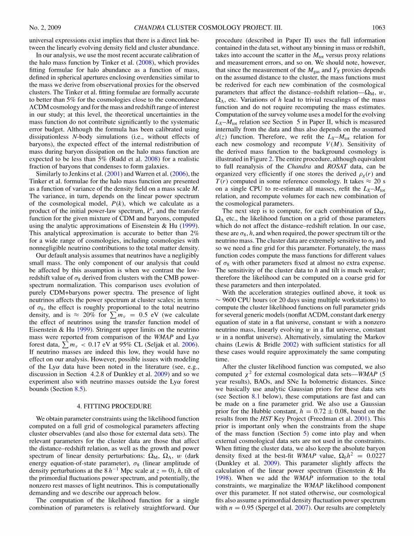
Figure 4. Comparison with other σ8 measurements. The solid region is our68% CL region reproduced from Figure 3 (this and all other confidence regionscorrespond to Δχ2 = 1, see footnote 13. Blue contours show the WMAP 3 and 5year results from Spergel et al. (2007) and Dunkley et al. (2009; dotted and solidcontours, respectively). For other measurements, we show the general directionof degeneracy as a solid line and a 68% uncertainty in σ8 at a representative valueof ΩM . Filled circles show the weak-lensing shear results from Hoekstra et al.(2006) and Fu et al. (2008; dashed and solid lines, respectively). Open circleshows results from a cluster sample with galaxy dynamics mass measurements(Rines et al. 2007). Finally, open square shows the results from Reiprich &Bohringer (2002, approximately the lower bound of recently published X-raycluster measurements).

degeneracy between σ8 and ΩM can be accurately describedas σ8 = 0.813(ΩM/0.25)−0.47. The ΩM range along this lineis constrained by the shape of the local mass function com-bined with the HST prior on the Hubble constant (Section 5).Including the high-redshift data, we obtain very similar re-sults. For example, for ΩM = 0.25, the total sample givesσ8 = 0.803 ± 0.0105, to be compared with σ8 = 0.813 ± 0.012from low-z clusters only. This implies that the σ8 measure-ment is dominated by the more accurate local cluster data, asexpected.

Systematic errors of the σ8 measurement are dominated by theuncertainties in the absolute mass calibration. To test the effectof these uncertainties, we changed the normalization of the massversus proxy relations by ±9% (our estimate of systematic errorsin the mass scale calibration, see Section 2). The effect, shownby the dotted contour in Figure 3, is to shift the estimated valuesof σ8 by ±0.02, just outside the statistical 68% CL uncertainties.This range can be considered as a systematic uncertainty in ourσ8 determination for a fixed ΩM.

Our cluster constraints on σ8 are more accurate (for afixed ΩM) than any other method, even including systematicerrors (Figure 4). It is encouraging that our results are in verygood agreement with recent results from other methods. Themeasurements based on lensing sheer surveys, cluster massfunction with Mtot estimated from galaxy dynamics, and WMAP(5 year results assuming flat ΛCDM cosmology) are all withintheir respective 68% CL uncertainties from our best fit. Thisindependently confirms that our calibration of the cluster massscale is not strongly biased. Furthermore, the present systematicerrors in the cluster analysis are smaller than the statisticalaccuracy provided by WMAP-5 and other methods. This allows

us to effectively use the σ8 information in the dark energyequation-of-state constraints (Section 8.3).

We now move to models where the crucial role is played bythe high-redshift cluster mass function data. The first case toconsider is combined constraints for ΩM and ΩΛ in the nonflatΛCDM cosmology. To better demonstrate what role the differentcomponents of the information provided by the cluster massfunction play in the combined constraints, we consider twocases: (1) when the full cluster mass function information isused, and (2) when the shape information is artificially removedthus leaving only the evolutionary information.

7. CONSTRAINTS FOR NONFLAT ΛCDM COSMOLOGY:ΩM − ΩΛ

In the first case, for each combination of parameters, wecompute the full likelihood for the low- and high-z massfunctions and add the HST prior on the Hubble constant (thisis necessary for effective use of the mass function shapeinformation, see Sections 4 and 5). We then marginalize thecombined likelihood over nonessential parameters (σ8 and h inthis case) keeping the primordial power-spectrum index fixedat the WMAP best-fit value, n = 0.95. Removal of the shapeinformation (our second case) is achieved by letting n vary andmarginalizing over it. This is approximately equivalent to usinga free shape parameter for the CDM power spectra, the approachoften used in earlier cluster studies (e.g., Borgani et al. 2001).Constraints for both cases were obtained for mass functionsestimated using all our three proxies, TX, Mgas, and YX .

The results are presented in Figures 5 and 6. First, wecan easily identify the role of using the mass function shapeinformation (illustrated for the Mgas and YX proxies). Clearly, itmostly breaks the degeneracies along the ΩM axis. The best-fitvalues and statistical uncertainties for ΩM are very close to thosederived from the shape of the local mass function (and nearlyidentical to those from the total sample, Section 5).

For a fixed ΩM, the observed evolution in the cluster massfunction provides a constraint on ΩΛ. Degeneracies in theΩM − ΩΛ plane provided by different mass proxies appliedto the same set of clusters differ because of the differentdistance dependences of the Mtot estimates via TX, Mgas, andYX (see below). Even without the shape information, evolutionin the YX and Mgas-based mass functions requires ΩΛ > 0at the 85% and 99.7% CL, respectively. Including the shapeinformation, we obtain ΩM = 0.28 ± 0.04, ΩΛ = 0.78 ± 0.25(and ΩΛ > 0 is required at the 99% CL) from the YX-basedanalysis. The evolution of the Mgas-based mass function givesΩM = 0.27 ± 0.04, ΩΛ = 0.83 ± 0.15, and ΩΛ > 0 at99.98% CL. The TX-based mass function does not stronglyconstrain ΩΛ but provides an independent measurement of ΩMwith almost no degeneracy with ΩΛ: ΩM = 0.34 ± 0.08, ingood agreement with the mass function shape results (and alsoprevious measurements based on the evolution of the clustertemperature function, see Henry 2004). In a flat ΛCDM model(the one with ΩM + ΩΛ = 1), the constraint is slightly tighter,ΩM = 0.30 ± 0.05.

Systematic uncertainties of the ΩΛ measurements are dom-inated by possible departures of evolution in the Mtot versusproxy relations. This issue is discussed in detail below inconnection with the dark energy equation-of-state constraint(Section 8.4); here we note only that the systematic uncertain-ties are approximately 50% of the purely statistical error barson the dark energy parameters (ΩΛ, w). Therefore, our clusterdata provide a clear independent confirmation for nonzero ΩΛ.


Figure 5. Constraints for nonflat ΛCDM cosmology from evolution of thecluster mass function. The results using only the evolution information (changein the number density of clusters between z = 0 and z ≈ 0.55) are shown in blueand green from the Mgas and TX-based total mass estimates. The degeneracies inthese cases are different because these proxies result in very different distancedependence of the estimated masses (see text for details). The constraints fromthe YX-based mass function are between those for Mgas and TX (Figure 6).Adding the shape of the mass function information breaks degeneracies withΩM, significantly improving constraints from Mgas and YX with little effect onthe TX results.

Comments on the role of geometric information in the clustermass function test. Cosmological constraints based on fitting thecluster mass function generally use not only information fromgrowth of the structure but also that from the distance–redshiftrelation because derivation of the high-z mass functions from thedata assumes the d(z) and E(z) functions. Quite generally, theestimated mass is a power-law function of these dependences,M ∝ d(z)β E(z)−ε. Different mass proxies have different βand ε, and thus combine the geometric and growth of structureinformation in different ways and lead to different degeneraciesin the derived cosmological parameters. We find that stronglydistance-dependent proxies (such as Mgas, see Paper II) areintrinsically more powerful in constraining the dark energyparameters (ΩΛ, w). By contrast, distance-independent proxiessuch as TX result in poor sensitivity to dark energy but insteadbetter constrain ΩM. This is well illustrated by the results inFigure 5. The Mgas-based estimates for Mtot result (if we ignorethe shape of the mass function information) in degeneracyapproximately along the line ΩM +ΩΛ = 1. In fact, the evolutionof the cluster mass functions derived from Mgas can be madebroadly consistent with the ΩM ≈ 1, ΩΛ ≈ 0 cosmology ifone allows for strong deviations from the CDM-type initialpower spectra (Nuza & Blanchard 2006). However, the massfunctions estimated from the temperatures of the same clustersare grossly inconsistent with such a cosmology, irrespectiveof the assumptions on the initial power spectrum (ΩM = 1is 8.3σ away from the best fit to the temperature-based massfunction, Figure 5). It is encouraging that the 68% CL regionsfor all three mass proxies overlap near the “concordance” pointat ΩM = 0.25–0.3 and ΩΛ = 0.7–0.75.

Figure 6. Same as Figure 5 but for YX-based mass estimates.

8. FLAT UNIVERSE WITH CONSTANT DARK ENERGYEQUATION OF STATE: w0 − ΩX

Next, we study constraints on a constant dark energy equationof state, w0 ≡ pX/ρX, in a spatially flat universe. The analysisusing cluster data only is equivalent to the ΩM − ΩΛ case(Section 7). We compute the likelihood for the cluster massfunctions on a grid of parameters: present dark energy densityΩX (= 1 − ΩM), w0, h, and σ8, then add the HST prior on theHubble constant (Section 4). Marginalization over nonessentialparameters, h and σ8, gives the likelihood as a function ofΩM and w0. We also obtain the equation-of-state constraintscombining our cluster data with the three external cosmologicaldata sets (following the reasoning of Dunkley et al. 2009, forthe choice of these data sets).

8.1. External Cosmological Data Sets

SN Ia. We use the distance moduli estimated for the Type Ia SNefrom the HST sample of Riess et al. (2007), SNLS survey (Astieret al. 2006), and ESSENCE survey (Wood-Vasey et al. 2007),combined with the nearby SN sample (we used a combinationof all these samples compiled by Davis et al. 2007). Calculationof the SN Ia component of the likelihood function for the givencosmological model is standard and can be found in any of theabove references.

Baryonic Acoustic Oscillations. Detection of the baryonicacoustic peak in the correlation function for large red galaxiesin the SDSS survey leads to a good measurement of thecombination

[dA(z)2

(cz)2 H (z)

]1/3√ΩMH 2

0

[ n

0.98

]0.35= 0.469 ± 0.017 (1)

at z = 0.35 (Eisenstein et al. 2005, “SDSS LRG sample”). Thisprior mostly constrains ΩM but has some sensitivity also to thedark energy equation of state.

A more recent measurement of the BAO peaks in thecombined SDSS and 2dF survey data is presented in Percival


et al. (2007a) who determine the BAO distance measure at tworedshifts (z = 0.2 and z = 0.35) instead of one in Eisensteinet al. (2005). These new data are somewhat in tension (∼ 2σ )with the SN+WMAP results (see, e.g., Figure 11 in Percival et al.2007a), which may artificially tighten the constraints when theBAO data are combined with SN Ia, WMAP, and clusters. Wechecked, however, that from the combination of SN Ia, WMAP,and SDSS-LRG BAO, we derive the parameter constraints thatare essentially equivalent to those in Komatsu et al. (2009), whoused the Percival et al. priors. Therefore, the choice of the BAOdata set is unimportant in the combined constraints.

WMAP-5. The likelihood for WMAP 5 year data is computedusing a simplified approach described in Section 5.4 of Komatsuet al. (2009). This involves a computation, for a given set ofcosmological parameters, of three CMB parameters—angularscale of the first acoustic peak, A; the so-called shift parameter,R; and the recombination redshift, z∗. The likelihood for theWMAP-5 data is then computed using the covariance matrix forA, R, and z∗ provided in Komatsu et al. This method is almost asaccurate as direct computation of the WMAP likelihood (Wang &Mukherjee 2007) but is much faster, which allowed us to explorethe entire multidimensional grid of the cosmological parametersinstead of running Markov chain simulations. One additionalnote is that to compute the CMB likelihood, we had to add theabsolute baryon density, Ωbh

2, to our usual set of cosmologicalparameters and then marginalize over it. The reason is that whilethe average baryon density has very little impact on the rest ofour analysis, the CMB data are very sensitive to Ωbh

2, thusany variation of h must be accompanied by the correspondingvariation of Ωb without which the computation of the CMBlikelihood would be inadequate.

The method outlined above recovers essentially the entire in-formation from the location and relative amplitudes of the peaksin the CMB power spectrum (Wang & Mukherjee 2007). Oneadditional piece of information is the absolute normalizationof the CMB power spectra, reflecting the amplitude of densityperturbations at the recombination redshift, z∗ ≈ 1090. Con-trasted with σ8 determined from our cluster data at z ≈ 0, itconstrains the total growth of density perturbations between theCMB epoch and the present, and thus is a powerful additionaldark energy constraint.

WMAP-5 Plus Local σ8. The WMAP team provides theamplitude of the curvature perturbations at the k = 0.02 Mpc−1

scale,Δ2

R = (2.21 ± 0.09) × 10−9. (2)

Section 5.5 in Komatsu et al. (2009) gives the prescription ofhow to predict this observable for a given set of cosmologicalparameters and σ8. A useful accurate fitting formula can also befound in Hu & Jain (2004):

ΔR ≈ σ8

1.79 × 104

(Ωbh

2

0.024

)1/3 (ΩMh2

0.14

)−0.563

× (7.808 h)(1−n)/2

(h

0.72

)−0.693 0.76

G0(3)

(we adjusted numerical coefficients to take into account thatthe Hu & Jain approximation uses the CMB amplitude atk = 0.05 Mpc−1 while the WMAP-5 results are reported fork = 0.02 Mpc−1). In this equation, G0 is the perturbationgrowth factor between the CMB redshift and the present,normalized to the growth function in the matter-dominated

Figure 7. Constraints on the present dark energy density ΩX and constantequation-of-state parameter w0 derived from cluster mass function evolution ina spatially flat universe. The results for Mgas and YX-based total mass estimatesare shown in red and blue, respectively. The inner solid red region shows theeffect of adding the mass function shape information (Section 5) to the evolutionof the Mgas-based mass function.

universe: G(z) ≡ (1 + z) δ(z)/δ(zCMB). This fitting formulahelps to understand the nature of the σ8 versus CMB amplitudeconstraint. The relation between σ8 and ΔR depends on theabsolute matter and baryon densities, ΩMh2 and Ωbh

2 (wellmeasured by the CMB data alone), and on the total growthfactor, G0, and the absolute value of the Hubble constant, h.Both of these quantities provide powerful constraints on anyparameterization of the dark energy equation of state (Hu 2005),and their combination does so as well.

Inclusion of this information in the total likelihood is straight-forward. Given the usual set of cosmological parameters (ΩX,w0, h) plus σ8, one computes

χ2CMBnorm = (

Δ2R × 109 − 2.21

)2/0.092, (4)

where ΔR can be obtained either from Equation (3) or asdescribed in Komatsu et al. (2009). The χ2

CMBnorm component isthen added to the cluster χ2 and the sum marginalized over σ8.

8.2. w0 from Cluster Data Only

Constraints on the present dark energy density ΩX and con-stant equation of state are presented in Figure 7. For comparison,we show separately the results derived only from the evolution ofthe Mgas and YX-based mass functions, and the effect of includ-ing the mass function shape information (Section 7 describesthe procedure for removing shape information from the clus-ter likelihood function). We do not consider here the TX-basedmass estimates because they provide little sensitivity to the darkenergy parameters. (Section 7). Just like in the ΩM − ΩΛ case,evolution of the Mgas and YX-based mass functions constrainsdifferent combinations of w0 and ΩX. The width of the confi-dence regions across the degeneracy direction is similar but thegas-based results are less inclined giving a little more sensitivityto w0 for a fixed dark energy density—Δw0 = ±0.17 from theMgas-based functions and Δw0 = ±0.26 from YX .


Figure 8. Comparison of the dark energy constraints from X-ray clusters andfrom other individual methods (SNe, BAOs, and WMAP).

Adding the mass function information combined with theHST prior on h breaks the degeneracy along the ΩX direction.For example, the ellipse in Figure 7 shows the 68% CL regionfrom fitting both the evolution and shape of the Mgas-based massfunction. The one-parameter confidence intervals in this caseare ΩX = 0.75 ± 0.04 and w0 = −1.14 ± 0.21. These resultscompare favorably with those from other individual methods—SNe, BAO, WMAP (Figure 8), although the SNe and CMBdata provide tighter constraints on w0 for a fixed ΩX. Thereal strength of the cluster data is, however, when they arecombined with the CMB and other cosmological data sets. Thecombined constraints are very similar for the Mgas and YX-basedcluster mass functions, and therefore we discuss only the formerhereafter.

8.3. w0 from the Combination of Clusters with Other Data

First, we consider a combination of the cluster data withthe WMAP distance priors (see Section 5.4 in Komatsu et al.2009). Cluster data bring information on growth of densityperturbations and normalized distances in the z 0.0–0.9interval, and—weakly—on the ΩMh parameter. Adding thisinformation reduces the WMAP-only uncertainties on w0 andΩX approximately by a factor of 2 (dark blue region in Figure 9):w0 = −1.08 ± 0.15, ΩX = 0.76 ± 0.04.

A much more significant improvement of the constraintsarises from the σ8 determination from low-redshift clusters (darkred region in Figure 9). Comparison of the local determination ofσ8 with the CMB normalization mostly provides a measurementof the total perturbation growth factor between zCMB and thepresent. This depends more sensitively on w0 than the evolutionof the cluster mass function because of, first, larger redshiftleverage, and second, because the perturbation amplitude athigh z is measured more accurately by CMB than by 37 clustersfrom the 400d survey.

Is it appropriate to use the σ8 versus CMB normalizationinformation in the dark energy constraints or does it requireunreasonable interpolation of the dark energy parameteriza-tion to high redshifts? We note in this regard that for any

Figure 9. Dark energy constraints in a flat universe from the combination of theCMB and cluster data (dark blue region). Adding the σ8 vs. CMB normalizationinformation significantly improves constraints on w0 for a fixed ΩX (inner redregion).

combination of the cosmological parameters in the vicinity ofthe “concordance” model, w0 −1, ΩX = 0.25–0.3, the uni-verse becomes matter dominated and enters the decelerationstage by z ∼ 1.5 − 2; the growth of perturbations is basicallyfixed after that at G(z) = 1. In other words, the CMB data canbe used to safely predict the amplitude of density perturbationsat z = 1.5–2 almost independently of the exact dark energyproperties. As long as it is appropriate to use a particular darkenergy parameterization in the z = 0–2 interval, it is thereforeappropriate to use the same model for the joint clusters+WMAPfit.

By itself, adding the σ8 information does not significantlyimprove the w0 and ΩX constraints (the total extent of the 1σconfidence regions is similar to the WMAP+evolution case),but the confidence region becomes much more degenerate withΩX (see the inner red region in Figure 9), which increases thepotential for improvement when we combine these results withother cosmological data sets, BAO and SNe.

The combined constraints from all four cosmological datasets are shown in Figure 10 (inner dark red region). The 68%one-parameter confidence intervals are ΩX = 0.740 ± 0.012and w0 = −0.991 ± 0.045. The importance of adding informa-tion from our cluster samples is illustrated by a factor of ∼ 1.5reduction of the measurement uncertainties with respect to theWMAP+SN+BAO data alone: we obtain w0 = −0.995 ± 0.067without clusters (dark blue region in Figure 10; these results areessentially identical to those reported in Komatsu et al. 2009).Perhaps more importantly, including the cluster data also re-duces systematic uncertainties by a similar amount (Section 8.4).

The best-fit values of the Hubble constant and σ8 fromthe combination of all data sets are h = 0.715 ± 0.012 andσ8 = 0.786 ± 0.011. These values are within 68% confidenceintervals of their determination by direct measurements (HSTKey Project results for h and fitting the low-z cluster massfunction for σ8). The best-fit combination of the dark energyparameters is also within the 1σ confidence regions for eachindividual data set included in the constraints (Figure 10).


Figure 10. Dark energy constraints in a flat universe from the combination ofall cosmological data sets. We find w0 = −0.991 ± 0.045 (±0.04 systematic)and ΩX = 0.740 ± 0.012, see Table 2 and Section 8.3.

Therefore, the best-fit cosmological model is a good fit tothe data. In particular, Figure 17 from Vikhlinin et al. (2009)shows that the mass function models computed in the ΛCDMcosmology (w0 = −1) provide a very good description of thedata.

8.4. Systematic Uncertainties in the w0 Measurements

We estimate the effect of known sources of systematics on thecosmological constraints by varying the corresponding individ-ual sets of data or internal relations (e.g., evolution in LX–Mtotentering the survey volume computations) within the estimated1σ interval. We assume, optimistically, that the current WMAPand BAO data are free from significant systematics (i.e., thatthey are smaller than statistical uncertainties), and consider sys-tematic errors only in the SN Ia and cluster data sets. In mostcases, a single source clearly dominates the systematic errorbudget for a particular measurement, so we report on only thosedominant sources.

The largest known source of systematic error in the SN Iaanalysis is the correction for extinction in host galaxies anduncertainties in intrinsic colors of SN Ia (e.g., Frieman et al.2008). As a measure of systematic uncertainty in the combinedSN sample, we use ±0.13 in w0 for fixed ΩX, quoted by Wood-Vasey et al. (2007). We implement these errors by computingthe SN likelihood in our experiments for (ΩX,w0 + 0.13) and(ΩX,w0 − 0.13) instead of (ΩX,w0).

8.4.1. Main Sources of Cluster Systematics

The largest sources of systematic errors in the cluster analysisare those in the normalization of the Mtot versus proxy relations.They can be separated into two almost independent components:(1) how accurately is the absolute cluster mass scale establishedby X-ray hydrostatic Mtot estimates in the low-redshift clusters,and (2) how accurately can we predict evolution in the Mtotversus proxy relations, i.e., the relative mass scale between low-and high-redshift clusters. The first component mainly affectsthe σ8 measurements and the associated dark energy constraints,

while the second component affects the results derived fromusing only evolution in the cluster mass function (those inFigure 7). Our estimates of the Mtot systematics are discussedextensively in Vikhlinin et al. (2009). For the absolute massscale (Mtot for fixed YX , TX, or Mgas) at z ≈ 0, we estimateΔMsys/M � 9% mainly from the comparison of the X-ray andweak-lensing mass estimates in representative samples. Thissource of error is implemented by changing the normalizationof the Mtot versus YX , Mgas, or TX relations at z = 0 by ±9%.For uncertainties in the evolution of the Mtot versus proxyrelations, we estimate ΔM/M ≈ 5% at z = 0.5, mainlyfrom the comparison of the prediction of different modelsdescribing observed small deviations of the cluster scalingrelations from self-similar predictions, and from the magnitudeof these deviations and corresponding corrections we apply tothe data. These uncertainties are implemented by multiplyingthe standard scaling relations by factors of (1 + z)±0.12.

Comparable to the evolution in the Mtot versus proxy relationare measurement uncertainties in the evolution factor for the LX–Mtot relation. We do not use LX to estimate the cluster masses,but the relation is required to compute the survey volume forthe high-z sample. The resulting volume uncertainty dependson the mass scale, and can become comparable to the Poissonerror for the comoving cluster number density (see Section 5.1.3in Vikhlinin et al. 2009). We tested how this influences thecosmological fit by varying the parameters of the LX–Mtotrelation within their measurement errors around the best fit (theevolution of LX for fixed Mtot in our model is parameterizedas E(z)γ and γ is measured to ±0.33; see Section 5.1.3 inVikhlinin et al. 2009).

Other sources of systematics in the cluster analysis (sum-marized in Vikhlinin et al. 2009) are negligible compared withthose outlined above. We verified also that uncertainties in theintrinsic scatter in the Mtot-proxy relations are not important.The main reason is that in the dark energy constraints, we usehigh-quality mass proxies (YX and Mgas), which should providemass estimates with small, 7%–10% scatter. Variations of thisscatter by up to ±50% with respect to the nominal values donot significantly change the best-fit cosmological parameters.This conclusion is seemingly different from Lima & Hu (2005)because in that paper, they consider proxies with larger scatter(the effect on the cosmological parameter constraints is pro-portional to scatter squared), and also they assumed that thenormalizations in the Mtot versus proxy relation are obtainedfrom self-calibration while we use direct mass measurementsfor a well observed subsample.

The variations of the best-fit parameters due to the systematicsdiscussed above are reported in Table 2 along with the dominantsource of error for each combination of cosmological data sets.For example, variations in the evolution of the Mtot–Mgas andMtot–YX relations affect the best fit to the cluster data only byΔw0 = ±0.1, while statistical uncertainties are ±0.2 to ±0.3for fixed ΩX (Section 8.2); unless the systematics in this caseare a factor of 2 larger than our estimates, they are unimportant.

8.4.2. Systematics in the Combined Constraints

The most interesting case to consider is the reduction in thesystematic errors from combining both SN and cluster data withthe WMAP and BAO priors. In the SN+CMB+BAO case, theSNe systematics cause variations in the best-fit w0 by ±0.076(reduced from ±0.13 for the SN-only case mainly by includ-ing WMAP priors). Cluster systematics affects the w0 con-straints from the clusters+WMAP+BAO combination by ±0.04


(dominated by the ±9% uncertainties in the absolute massscale). The influence of both sources of error is significantlyreduced in the combined constraints. We find that the best fit w0from SN+clusters+WMAP+BAO is affected by ±0.022 by SNsystematics, and by ±0.033 by cluster systematics. The total sys-tematic error in the combined constraint is thus Δw0 = ±0.04,almost a factor of 2 reduction from ±0.076 achievable withoutclusters.

We also note that if we significantly underestimate the clustersystematics, the most likely direction is that the cluster totalmasses are underestimated.14 If the cluster Mtot are revised high,this would lead to an increase in the derived σ8, and decreasein w0 when cluster data are combined with the CMB priors.Dark energy models predicting the equation-of-state parametersignificantly above w0 = −1 will be even less consistent withobservations in this case.

8.4.3. Prospects for Further Reduction of Systematic Errors

It is reassuring that all sources of systematic errors weconsidered affect the dark energy equation-of-state constraintswithin the statistical measurement errors. This implies that whilesystematic errors are important, they do not yet dominate thecurrent error budget. The situation will reverse in the future asthe data sets expand. More effort will be needed then to reducethe systematics still further. We briefly outline the prospectsfor reducing the cluster-related systematics. Some of this willhappen automatically as the high-z surveys become deeper andcover a larger area. For example, the V (M) uncertainties forour range of redshifts can be eliminated simply by decreasingthe flux threshold by a factor of ∼ 4 compared with the 400dlimit, making the sample volume-limited; such an extensionwill provide also a more accurate measurement of the LX–Mtotrelation. The absolute calibration of Mtot in low-z clusters can beimproved by constraining sources of nonthermal pressure (e.g.,if turbulence is of any importance for the Mtot estimates, it iseasily detectable with an X-ray microcalorimeter), or throughstacked weak-lensing analysis (e.g., measuring average lensingshear profiles for a large set of clusters with the same YX).To improve limits on nonstandard evolution in the Mtot versusproxy relations, we cannot use direct mass measurements ofthe high-z objects because they will be degenerate with theassumed distance–redshift relation. Instead, we should improvereliability of numerical models for cluster evolution. The biggestuncertainties in these models at present are related to theprocesses of gas cooling and star formation, and also to energyfeedback from the central AGN. The strategy for future progresscan be based on the fact that these processes most stronglyaffect cluster cores, which we do not use for the mass estimates.We can, therefore, use the data from the central regions tobracket a likely range of uncertainty in the model predictionsfor the cluster outer regions, where we derive the Mtot proxies.However, even with the current estimated uncertainties, thesamples can grow by a factor of ∼ 4 before the systematics startto dominate. Ultimately, as the cluster surveys detect ∼ 104

clusters with accurately measured X-ray parameters, the so-called self-calibration techniques (Majumdar & Mohr 2004;

14 The X-ray hydrostatic analysis includes only the gas thermal pressure andassumes that the cluster gas body is close to being spherically symmetric. Thepresence of additional components in the pressure, clumpiness, and turbulentmotions in the gas all lead to underestimation of Mtot derived from X-ray data.Probably the only possibility for overestimation of Mtot in the X-ray analysis isa gross miscalibration of the Chandra spectral response, for which strongexperimental limits are available.

Lima & Hu 2004) can be employed to further constrain theevolution in the Mtot versus proxy relations.

8.5. Effects of Nonzero Neutrino Mass

If light neutrinos have masses in the range of a few 0.1 eV,they become nonrelativistic between zCMB and z = 0, and thistransition produces distortions in the matter perturbations powerspectrum relative to the prediction of the pure CDM+baryonsmodel. Using approximations of the transfer function fromEisenstein & Hu (1999), it is easy to verify that the effectis approximately proportional to the total mass of neutrinos(more exactly, to

∑mν/ΩM), and the rms fluctuations at cluster

scales today are suppressed by approximately 20% if∑

mν =0.5 eV and ΩM = 0.26. This effect is far outside the mea-surement uncertainties in σ8 from clusters (we quote systematicerrors of 3% from uncertainties in the Mtot calibration and sta-tistical uncertainties are even smaller, see Table 1). Therefore,neutrino masses in this range (1) may affect the dark energyconstraints when cluster data are combined with WMAP (be-cause they will effectively change the relation between σ8 andthe CMB normalization, Equation (3)), and (2) can be tightlyconstrained by our cluster data.

To test the effect of neutrinos, we ran an additional set ofmodels in which the total neutrino mass was allowed to varybetween 0 and 1 eV. For simplicity, we assumed that there arethree neutrino species with the same mass, but the final resultsare not very sensitive to this assumption. The only componentof our procedure, which is significantly affected by the nonzeroneutrino mass is contrasting the cluster-derived σ8 with theWMAP normalization of the CMB power spectrum. We canno longer rely on Equation (3) and should instead use the fullprocedure described in Section 5.5 of Komatsu et al. (2009).Otherwise, the analysis is equivalent to the

∑mν = 0 case.

The likelihood for all cosmological data sets was computedon our usual grid plus

∑mν as an additional free parameter,

and then marginalized over ΩX, h, and σ8. Finally, we tookinto account that a combination of WMAP, BAO, and SN dataprovides some sensitivity to the neutrino mass through the so-called early integrated Sachs-Wolfe effect (see discussion inSection 6.1.3 of Komatsu et al. 2009, and references therein).From this analysis, Komatsu et al. derive a 95% upper limit of∑

mν < 0.66 eV. Since our procedure of using WMAP priors(Section 8.1) ignores this additional information, we includedit approximately by adding a Gaussian prior

∑mν = 0 ± 0.33

eV to the final marginalized likelihood.The derived constraints on

∑mν and w0 are shown in

Figure 11. As expected, when the σ8 versus CMB normalizationconstraint is added, there is a degeneracy between the best-fitw0 and the total neutrino mass. If we were using only clustersand WMAP, the degeneracy would approximately follow theline w0 + 1 = −0.4

∑mν and would extend to

∑mν ≈ 1.3 eV

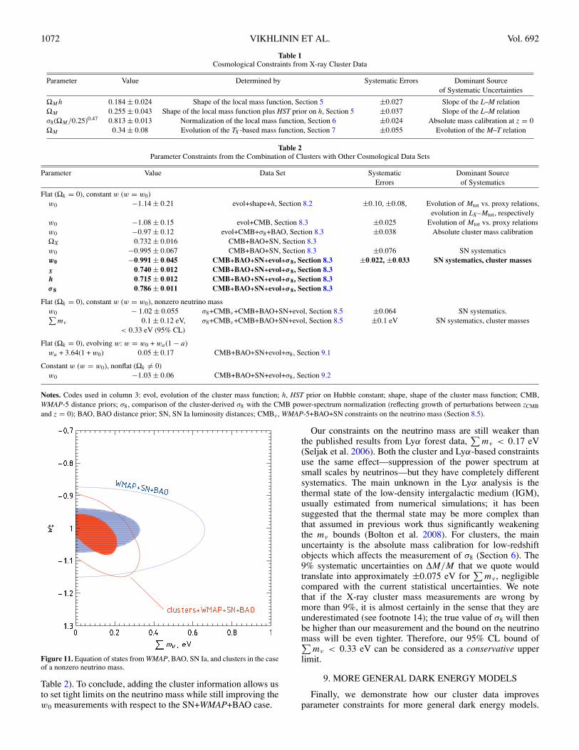
(the WMAP-only bound on the neutrino mass, Dunkley et al.2009). This degeneracy is broken, however, when we add theBAO and SN information: low values of w0 required by clus-ters+CMB for high values of the neutrino mass are inconsistentwith these two data sets. Therefore, a combination of all fourdata sets can be used to constrain both w0 and neutrino mass.The best-fit value is

∑mν = 0.10±0.12 eV, with a 95% CL up-

per limit of∑

mν < 0.33 eV. This limit is significantly tighterthan that is achievable without clusters (< 0.66 eV at 95% CL).The constraint on w0 degrades somewhat compared with themν = 0 case: w0 = −1.02 ± 0.055 (compared with ±0.045 formν = 0), but is still better than ±0.067 without clusters (see


Table 1Cosmological Constraints from X-ray Cluster Data

Parameter Value Determined by Systematic Errors Dominant Sourceof Systematic Uncertainties

ΩMh 0.184 ± 0.024 Shape of the local mass function, Section 5 ±0.027 Slope of the L–M relationΩM 0.255 ± 0.043 Shape of the local mass function plus HST prior on h, Section 5 ±0.037 Slope of the L–M relationσ8(ΩM/0.25)0.47 0.813 ± 0.013 Normalization of the local mass function, Section 6 ±0.024 Absolute mass calibration at z = 0ΩM 0.34 ± 0.08 Evolution of the TX-based mass function, Section 7 ±0.055 Evolution of the M–T relation

Table 2Parameter Constraints from the Combination of Clusters with Other Cosmological Data Sets

Parameter Value Data Set Systematic Dominant SourceErrors of Systematics

Flat (Ωk = 0), constant w (w = w0)w0 −1.14 ± 0.21 evol+shape+h, Section 8.2 ±0.10, ±0.08, Evolution of Mtot vs. proxy relations,

evolution in LX–Mtot, respectivelyw0 −1.08 ± 0.15 evol+CMB, Section 8.3 ±0.025 Evolution of Mtot vs. proxy relationsw0 −0.97 ± 0.12 evol+CMB+σ8+BAO, Section 8.3 ±0.038 Absolute cluster mass calibrationΩX 0.732 ± 0.016 CMB+BAO+SN, Section 8.3w0 −0.995 ± 0.067 CMB+BAO+SN, Section 8.3 ±0.076 SN systematicsw0 −0.991 ± 0.045 CMB+BAO+SN+evol+σ 8, Section 8.3 ±0.022, ±0.033 SN systematics, cluster masses

X 0.740 ± 0.012 CMB+BAO+SN+evol+σ 8, Section 8.3

h 0.715 ± 0.012 CMB+BAO+SN+evol+σ 8, Section 8.3

σ 8 0.786 ± 0.011 CMB+BAO+SN+evol+σ 8, Section 8.3

Flat (Ωk = 0), constant w (w = w0), nonzero neutrino massw0 − 1.02 ± 0.055 σ8+CMBν+CMB+BAO+SN+evol, Section 8.5 ±0.064 SN systematics.∑

mν 0.1 ± 0.12 eV, σ8+CMBν+CMB+BAO+SN+evol, Section 8.5 ±0.1 eV SN systematics, cluster masses< 0.33 eV (95% CL)

Flat (Ωk = 0), evolving w: w = w0 + wa(1 − a)wa + 3.64(1 + w0) 0.05 ± 0.17 CMB+BAO+SN+evol+σ8, Section 9.1

Constant w (w = w0), nonflat (Ωk �= 0)w0 −1.03 ± 0.06 CMB+BAO+SN+evol+σ8, Section 9.2

Notes. Codes used in column 3: evol, evolution of the cluster mass function; h, HST prior on Hubble constant; shape, shape of the cluster mass function; CMB,WMAP-5 distance priors; σ8, comparison of the cluster-derived σ8 with the CMB power-spectrum normalization (reflecting growth of perturbations between zCMB

and z = 0); BAO, BAO distance prior; SN, SN Ia luminosity distances; CMBν , WMAP-5+BAO+SN constraints on the neutrino mass (Section 8.5).

Figure 11. Equation of states from WMAP, BAO, SN Ia, and clusters in the caseof a nonzero neutrino mass.

Table 2). To conclude, adding the cluster information allows usto set tight limits on the neutrino mass while still improving thew0 measurements with respect to the SN+WMAP+BAO case.

Our constraints on the neutrino mass are still weaker thanthe published results from Lyα forest data,

∑mν < 0.17 eV

(Seljak et al. 2006). Both the cluster and Lyα-based constraintsuse the same effect—suppression of the power spectrum atsmall scales by neutrinos—but they have completely differentsystematics. The main unknown in the Lyα analysis is thethermal state of the low-density intergalactic medium (IGM),usually estimated from numerical simulations; it has beensuggested that the thermal state may be more complex thanthat assumed in previous work thus significantly weakeningthe mν bounds (Bolton et al. 2008). For clusters, the mainuncertainty is the absolute mass calibration for low-redshiftobjects which affects the measurement of σ8 (Section 6). The9% systematic uncertainties on ΔM/M that we quote wouldtranslate into approximately ±0.075 eV for

∑mν , negligible

compared with the current statistical uncertainties. We notethat if the X-ray cluster mass measurements are wrong bymore than 9%, it is almost certainly in the sense that they areunderestimated (see footnote 14); the true value of σ8 will thenbe higher than our measurement and the bound on the neutrinomass will be even tighter. Therefore, our 95% CL bound of∑

mν < 0.33 eV can be considered as a conservative upperlimit.

9. MORE GENERAL DARK ENERGY MODELS

Finally, we demonstrate how our cluster data improvesparameter constraints for more general dark energy models.


Figure 12. Constrains on evolving equation of state, w(z) = w0 + waz/(1 + z),in a flat universe.

We consider two cases —evolving equation of state, w =w(z), and constant equation of state in a nonflat universe.The results are presented less completely than for the caseof constant w in a flat universe. We also do not discusssystematic uncertainties separately for these cases; we checkedthat the importance of different sources of systematics and theirfraction of statistical uncertainties is approximately the sameas reported in Section 8.4 for the constant w, a flat universecase.

9.1. w(z) in a Flat Universe

We consider an often used parameterization of the equation-of-state evolution in which w changes linearly with the ex-pansion factor, w(a) = w0 + wa(1 − a), or equivalently,w(z) = w0 + waz/(1 + z). We do not consider more complexparameterizations because constraints on the evolution term arestill weak, and because neither parameterization has a clearphysical motivation.

The likelihood function is computed on the ΩM, w0, wa, h,σ8 grid and then marginalized over ΩM, h, and σ8, leading toconstraints in the w0 −wa plane shown in Figure 12. Constraintson wa are weak with or without clusters. For example, themodel with w0 = −1.2 and wa = 1 (leading to w = −0.7 byz = 1) is perfectly consistent with the data. However, clustersmake the confidence region substantially narrower (improvewa constraints for a fixed w0). A cosmological constant model(w0 = −1, wa = 0) is still consistent with the data.

Finally, we note that in either case, the degeneracy between w0and wa is almost linear, wa = A + B w0. For such degeneracies,constraints on constant w are equivalent to those for evolvingw at the pivot redshift, ap = (1 + zp)−1 = 1 + 1/B (Hu &Jain 2004). From the slopes of degeneracies in Figure 12, wefind zp ≈ 0.29 without clusters and zp ≈ 0.38 when clusterinformation is included. Therefore, our combined constraintson constant w (Section 8) can also be interpreted as those forevolving w at this pivot redshift.

Figure 13. Equation-of-state constrains from WMAP, BAO, SN Ia, and clustersin the case of a nonflat universe. We find w0 = −1.03 ± 0.06 and Ωk =−0.008 ± 0.009 with all the data combined.

9.2. w0 in a Nonflat Universe

The final case we consider is constant w in a nonflat universe.The cosmological grid in this case is (Ωk, ΩM, w0, h, σ8) withthe requirement that the dark energy density is ΩX = 1 −ΩM − Ωk . The likelihood is marginalized over ΩM, h, σ8, andthe constraints on Ωk and w0 are shown in Figure 13. Includingclusters does not noticeably improve the measurement of Ωk; byfar the most significant contribution to the Ωk constraint is fromthe combination of WMAP and BAO data (Komatsu et al. 2009).However, clusters do substantially improve the equation-of-statemeasurement: w0 = −1.03 ± 0.06 to be compared with ±0.085without clusters. A flat ΛCDM model (Ωk = 0, w0 = −1) isstill consistent with the data within 68% CL.

10. SUMMARY AND CONCLUSIONS

We presented constraints on the cosmological parametersfrom a new measurement on the galaxy cluster mass function inthe redshift range z = 0–0.9. All major sources of informationcontained in the cluster mass function—its overall normalizationand slope at z = 0, and evolution at high redshifts—aredetermined with our new data with a higher statistical accuracyand smaller systematic errors than before. This leads to muchimproved and more reliable constraints on the cosmologicalparameters.

From the normalization of the mass function estimated atlow redshifts, we derive the σ8 parameter degenerate withΩM: σ8(ΩM/0.25)0.47 = 0.813 ± 0.013 (stat) ±0.024 (sys).The slope of the low-z mass function is a measure of ΩMh:ΩMh = 0.184 ± 0.037; combined with the HST prior on h, thisis an independent measurement of ΩM = 0.255 ± 0.043. Thematter density can be independently measured with our clusterdata using the evolution of the temperature function, yieldingconsistent results, ΩM = 0.30±0.05 in a flat ΛCDM model and0.34 ± 0.08 in a general cosmology.

Evolution of the mass functions between z = 0 and 0.5(median redshift for our high-z sample) constrains ΩΛ = 0.83±


0.15 in nonflat ΛCDM cosmology, or the dark energy equation-of-state parameter, w0 = −1.14 ± 0.21, in a spatially flatuniverse. Inclusion of the information provided by our clusterdata also significantly improves the equation-of-state constraintsobtained from the combination of multiple cosmological datasets. For example, by combining the 5 year WMAP, most recentSNe measurements, and detection of BAOs in the SDSS withour cluster data, we obtain w0 = −0.991 ± 0.045 (stat) ±0.040(sys); both the statistical and systematic errors in the combinedconstraint are a factor of 1.5–2 smaller than those withoutclusters. Including cluster information also improves results foran evolving equation-of-state parameter and for constant w ina nonflat universe. A spatially flat ΛCDM model is within the68% CL interval from the best fit in all cases that we tested.

A good agreement between the geometric and growth ofstructure-based measurements of w in principle can be usedto place limits on modified gravity theories which attempt toexplain cosmic acceleration without dark energy (e.g., Wanget al. 2007). When self-consistent models of nonlinear collapsein such theories become available, it should be straightforwardto use our cluster data in such tests also.

Comparison of the power-spectrum normalization at z =0 obtained from clusters with the amplitude of the CMBfluctuations is a sensitive measure of the masses of lightneutrinos. We constrain

∑mν < 0.33 eV at 95% CL, at the

expense of slightly weakening the measurement of w0 obtainedassuming that the neutrino masses are negligibly small.

To facilitate the use of our cluster results in our cosmologicalstudies, we provide at the project Web site15 machine-readabletables of the likelihood function computed on several cosmo-logical grids.

We thank Jeremy Tinker for providing his mass functionmodel results prior to publication. We also thank W. Hu,O. Gnedin, M. Markevitch, and H. Tananbaum for many use-ful discussions, and D. Spergel and A. Loeb for commentson the manuscript. Financial support was provided by NASAgrants and contracts NAG5-9217, GO5-6120A, NAS8-39073(A.V., W.R.F., C.J., S.S.M.), GO5-6120C (H.E.); NSF grantsAST-0239759 and AST-0507666, NASA grant NAG5-13274and the Kavli Institute for Cosmological Physics at the Univer-sity of Chicago (A.K.); Sherman Fairchild Foundation (D.N.);FONDAP Centro de Astrofisica (H.Q.); Russian Foundationfor Basic Research grants RFFI 05-02-16540 and RFFI 08-02-00974 and the RAS program OFN-17 (R.B. and A.V.).

REFERENCES

Albrecht, A., et al. 2006, arXiv:astro-ph/0609591Allen, S. W., Rapetti, D. A., Schmidt, R. W., Ebeling, H., Morris, R. G., &

Fabian, A. C. 2008, MNRAS, 383, 879Astier, P., et al. 2006, A&A, 447, 31Bardeen, J. M., Bond, J. R., Kaiser, N., & Szalay, A. S. 1986, ApJ, 304, 15Bolton, J. S., Viel, M., Kim, T.-S., Haehnelt, M. G., & Carswell, R. F.

2008, MNRAS, 386, 1131Bond, J. R., Cole, S., Efstathiou, G., & Kaiser, N. 1991, ApJ, 379, 440Borgani, S., et al. 2001, ApJ, 561, 13Burenin, R. A., Vikhlinin, A., Hornstrup, A., Ebeling, H., Quintana, H., &

Mescheryakov, A. 2007, ApJS, 172, 561 (Paper I)Cash, W. 1976, A&A, 52, 307Cash, W. 1979, ApJ, 228, 939Cole, S., et al. 2005, MNRAS, 362, 505

15 http://hea-www.harvard.edu/400d/CCCP

Davis, T. M., et al. 2007, ApJ, 666, 716Dunkley, J., et al. 2009, ApJS, 180, 306Ebeling, H., Edge, A. C., & Henry, J. P. 2001, ApJ, 553, 668Eisenstein, D. J., & Hu, W. 1998, ApJ, 496, 605Eisenstein, D. J., & Hu, W. 1999, ApJ, 511, 5Eisenstein, D. J., et al. 2005, ApJ, 633, 560Evrard, A. E., et al. 2002, ApJ, 573, 7Freedman, W. L., et al. 2001, ApJ, 553, 47Frenk, C. S., White, S. D. M., Efstathiou, G., & Davis, M. 1990, ApJ, 351, 10Frieman, J., Turner, M., & Huterer, D. 2008, ARA&A, 46, 385Fu, L., et al. 2008, A&A, 479, 9Grossi, M., Dolag, K., Branchini, E., Matarrese, S., & Moscardini, L. 2007,

MNRAS, 382, 1261Henry, J. P. 2004, ApJ, 609, 603Henry, J. P., & Arnaud, K. A. 1991, ApJ, 372, 410Hoekstra, H. 2007, MNRAS, 379, 317Hoekstra, H., et al. 2006, ApJ, 647, 116Hu, W. 2005, in ASP Conf. Ser. 339, Observing Dark Energy, ed. S. C. Wolff,

& T. R. Lauer (San Francisco, CA: ASP), 215Hu, W., & Jain, B. 2004, Phys. Rev. D, 70, 043009Hu, W., & Kravtsov, A. V. 2003, ApJ, 584, 702Huterer, D., & White, M. 2002, ApJ, 578, L95Jeltema, T. E., Hallman, E. J., Burns, J. O., & Motl, P. M. 2008, ApJ, 681, 167Jenkins, A., Frenk, C. S., White, S. D. M., Colberg, J. M., Cole, S., Evrard, A.

E., Couchman, H. M. P., & Yoshida, N. 2001, MNRAS, 321, 372Kaiser, N. 1984, ApJ, 284, L9Komatsu, E., et al. 2009, ApJS, 180, 330Kravtsov, A. V., Vikhlinin, A., & Nagai, D. 2006, ApJ, 650, 128Lee, J., & Shandarin, S. F. 1998, ApJ, 500, 14Lee, J., & Shandarin, S. F. 1999, ApJ, 517, L5Lewis, A., & Bridle, S. 2002, Phys. Rev. D, 66, 103511Lilje, P. B. 1992, ApJ, 386, L33Lima, M., & Hu, W. 2004, Phys. Rev. D, 70, 043504Lima, M., & Hu, W. 2005, Phys. Rev. D, 72, 043006Linder, E. V., & Jenkins, A. 2003, MNRAS, 346, 573Majumdar, S., & Mohr, J. J. 2004, ApJ, 613, 41Mantz, A., Allen, S. W., Ebeling, H., & Rapetti, D. 2008, MNRAS, 387, 1179Nagai, D., Vikhlinin, A., & Kravtsov, A. V. 2007, ApJ, 655, 98Nuza, S. E., & Blanchard, A. 2006, A&A, 452, 47Percival, W. J., Cole, S., Eisenstein, D. J., Nichol, R. C., Peacock, J. A., Pope,

A. C., & Szalay, A. S. 2007a, MNRAS, 381, 1053Percival, W. J., et al. 2007b, ApJ, 657, 51Percival, W. J., et al. 2007c, ApJ, 657, 645Perlmutter, S., et al. 1999, ApJ, 517, 565Pierpaoli, E., Borgani, S., Scott, D., & White, M. 2003, MNRAS, 342, 163Press, W. H., & Schechter, P. 1974, ApJ, 187, 425Rasia, E., et al. 2006, MNRAS, 369, 2013Reiprich, T. H., & Bohringer, H. 2002, ApJ, 567, 716Riess, A. G., et al. 1998, AJ, 116, 1009Riess, A. G., et al. 2007, ApJ, 659, 98Rines, K., Diaferio, A., & Natarajan, P. 2007, ApJ, 657, 183Rudd, D. H., Zentner, A. R., & Kravtsov, A. V. 2008, ApJ, 672, 19Schuecker, P., Bohringer, H., Collins, C. A., & Guzzo, L. 2003, A&A, 398, 867Seljak, U., Slosar, A., & McDonald, P. 2006, J. Cosmol. Astropart. Phys., 10,

14Sheth, R., Mo, H., & Tormen, G. 2001, MNRAS, 323, 1Spergel, D. N., et al. 2007, ApJS, 170, 377Stanek, R., Evrard, A. E., Bohringer, H., Schuecker, P., & Nord, B. 2006, ApJ,

648, 956Tegmark, M., et al. 2004, Phys. Rev. D, 69, 103501Tinker, J. L., Kravtsov, A. V., Klypin, A., Abazajian, K., Warren, M. S., Yepes,

G., Gottlober, S., & Holz, D. E. 2008, ApJ, 688, 709Vikhlinin, A., Kravtsov, A., Forman, W., Jones, C., Markevitch, M., Murray, S.

S., & Van Speybroeck, L. 2006, ApJ, 640, 691Vikhlinin, A., et al. 2009, ApJ, 692, 1033Wang, S., Hui, L., May, M., & Haiman, Z. 2007, Phys. Rev. D, 76, 063503Wang, Y., & Mukherjee, P. 2007, Phys. Rev. D, 76, 103533Warren, M. S., Abazajian, K., Holz, D. E., & Teodoro, L. 2006, ApJ, 646,

881White, S. D. M., Efstathiou, G., & Frenk, C. S. 1993, MNRAS, 262, 1023Wood-Vasey, W. M., et al. 2007, ApJ, 666, 694Zhang, Y.-Y., Finoguenov, A., Bohringer, H., Kneib, J.-P., Smith, G. P., Kneissl,

R., Okabe, N., & Dahle, H. 2008, A&A, 482, 451

http://www.arxiv.org/abs/astro-ph/0609591

http://dx.doi.org/10.1111/j.1365-2966.2007.12610.x

http://adsabs.harvard.edu/cgi-bin/bib_query?2008MNRAS.383..879A

http://adsabs.harvard.edu/cgi-bin/bib_query?2008MNRAS.383..879A

http://dx.doi.org/10.1051/0004-6361:20054185

http://adsabs.harvard.edu/cgi-bin/bib_query?2006A&A...447...31A

http://adsabs.harvard.edu/cgi-bin/bib_query?2006A&A...447...31A

http://dx.doi.org/10.1086/164143

http://adsabs.harvard.edu/cgi-bin/bib_query?1986ApJ...304...15B


http://dx.doi.org/10.1111/j.1365-2966.2008.13114.x

http://adsabs.harvard.edu/cgi-bin/bib_query?2008MNRAS.386.1131B

http://adsabs.harvard.edu/cgi-bin/bib_query?2008MNRAS.386.1131B

http://dx.doi.org/10.1086/170520

http://adsabs.harvard.edu/cgi-bin/bib_query?1991ApJ...379..440B

http://adsabs.harvard.edu/cgi-bin/bib_query?1991ApJ...379..440B

http://dx.doi.org/10.1086/323214



http://dx.doi.org/10.1086/519457

http://adsabs.harvard.edu/cgi-bin/bib_query?2007ApJS..172..561B

http://adsabs.harvard.edu/cgi-bin/bib_query?2007ApJS..172..561B

http://adsabs.harvard.edu/cgi-bin/bib_query?1976A&A....52..307C

http://adsabs.harvard.edu/cgi-bin/bib_query?1976A&A....52..307C

http://dx.doi.org/10.1086/156922

http://adsabs.harvard.edu/cgi-bin/bib_query?1979ApJ...228..939C

http://adsabs.harvard.edu/cgi-bin/bib_query?1979ApJ...228..939C

http://dx.doi.org/10.1111/j.1365-2966.2005.09318.x

http://adsabs.harvard.edu/cgi-bin/bib_query?2005MNRAS.362..505C

http://adsabs.harvard.edu/cgi-bin/bib_query?2005MNRAS.362..505C

http://hea-www.harvard.edu/400d/CCCP

http://dx.doi.org/10.1086/519988

http://adsabs.harvard.edu/cgi-bin/bib_query?2007ApJ...666..716D

http://adsabs.harvard.edu/cgi-bin/bib_query?2007ApJ...666..716D

http://dx.doi.org/10.1088/0067-0049/180/2/306

http://dx.doi.org/10.1086/320958

http://adsabs.harvard.edu/cgi-bin/bib_query?2001ApJ...553..668E


http://dx.doi.org/10.1086/305424



http://dx.doi.org/10.1086/306640

http://dx.doi.org/10.1086/466512



http://dx.doi.org/10.1086/340551

http://adsabs.harvard.edu/cgi-bin/bib_query?2002ApJ...573....7E

http://adsabs.harvard.edu/cgi-bin/bib_query?2002ApJ...573....7E

http://dx.doi.org/10.1086/320638

http://adsabs.harvard.edu/cgi-bin/bib_query?2001ApJ...553...47F


http://dx.doi.org/10.1086/168439



http://dx.doi.org/10.1146/annurev.astro.46.060407.145243

http://adsabs.harvard.edu/cgi-bin/bib_query?2008ARA&A..46..385F

http://adsabs.harvard.edu/cgi-bin/bib_query?2008ARA&A..46..385F

http://dx.doi.org/10.1051/0004-6361:20078522

http://adsabs.harvard.edu/cgi-bin/bib_query?2008A&A...479....9F

http://adsabs.harvard.edu/cgi-bin/bib_query?2008A&A...479....9F

http://adsabs.harvard.edu/cgi-bin/bib_query?2007MNRAS.382.1261G

http://adsabs.harvard.edu/cgi-bin/bib_query?2007MNRAS.382.1261G

http://dx.doi.org/10.1086/421336

http://adsabs.harvard.edu/cgi-bin/bib_query?2004ApJ...609..603H


http://dx.doi.org/10.1086/169987



http://dx.doi.org/10.1111/j.1365-2966.2007.11951.x

http://adsabs.harvard.edu/cgi-bin/bib_query?2007MNRAS.379..317H

http://adsabs.harvard.edu/cgi-bin/bib_query?2007MNRAS.379..317H

http://dx.doi.org/10.1086/503249



http://adsabs.harvard.edu/cgi-bin/bib_query?2005ASPC..339..215H

http://dx.doi.org/10.1103/PhysRevD.70.043009

http://adsabs.harvard.edu/cgi-bin/bib_query?2004PhRvD..70D3009H

http://adsabs.harvard.edu/cgi-bin/bib_query?2004PhRvD..70D3009H

http://dx.doi.org/10.1086/345846



http://dx.doi.org/10.1086/344699

http://adsabs.harvard.edu/cgi-bin/bib_query?2002ApJ...578L..95H

http://adsabs.harvard.edu/cgi-bin/bib_query?2002ApJ...578L..95H

http://dx.doi.org/10.1086/587502

http://adsabs.harvard.edu/cgi-bin/bib_query?2008ApJ...681..167J

http://adsabs.harvard.edu/cgi-bin/bib_query?2008ApJ...681..167J

http://dx.doi.org/10.1046/j.1365-8711.2001.04029.x

http://adsabs.harvard.edu/cgi-bin/bib_query?2001MNRAS.321..372J

http://adsabs.harvard.edu/cgi-bin/bib_query?2001MNRAS.321..372J

http://dx.doi.org/10.1086/184341

http://adsabs.harvard.edu/cgi-bin/bib_query?1984ApJ...284L...9K

http://adsabs.harvard.edu/cgi-bin/bib_query?1984ApJ...284L...9K

http://dx.doi.org/10.1088/0067-0049/180/2/330

http://dx.doi.org/10.1086/506319

http://adsabs.harvard.edu/cgi-bin/bib_query?2006ApJ...650..128K

http://adsabs.harvard.edu/cgi-bin/bib_query?2006ApJ...650..128K

http://dx.doi.org/10.1086/305710

http://adsabs.harvard.edu/cgi-bin/bib_query?1998ApJ...500...14L

http://adsabs.harvard.edu/cgi-bin/bib_query?1998ApJ...500...14L

http://dx.doi.org/10.1086/312012


http://adsabs.harvard.edu/cgi-bin/bib_query?2002PhRvD..66j3511L

http://adsabs.harvard.edu/cgi-bin/bib_query?2002PhRvD..66j3511L

http://dx.doi.org/10.1086/186286

http://adsabs.harvard.edu/cgi-bin/bib_query?1992ApJ...386L..33L

http://adsabs.harvard.edu/cgi-bin/bib_query?1992ApJ...386L..33L


http://adsabs.harvard.edu/cgi-bin/bib_query?2004PhRvD..70D3504L

http://adsabs.harvard.edu/cgi-bin/bib_query?2004PhRvD..70D3504L


http://dx.doi.org/10.1046/j.1365-2966.2003.07112.x

http://adsabs.harvard.edu/cgi-bin/bib_query?2003MNRAS.346..573L

http://adsabs.harvard.edu/cgi-bin/bib_query?2003MNRAS.346..573L

http://dx.doi.org/10.1086/422829

http://adsabs.harvard.edu/cgi-bin/bib_query?2004ApJ...613...41M

http://adsabs.harvard.edu/cgi-bin/bib_query?2004ApJ...613...41M

http://dx.doi.org/10.1111/j.1365-2966.2008.13311.x

http://adsabs.harvard.edu/cgi-bin/bib_query?2008MNRAS.387.1179M

http://adsabs.harvard.edu/cgi-bin/bib_query?2008MNRAS.387.1179M

http://dx.doi.org/10.1086/509868

http://adsabs.harvard.edu/cgi-bin/bib_query?2007ApJ...655...98N

http://adsabs.harvard.edu/cgi-bin/bib_query?2007ApJ...655...98N

http://dx.doi.org/10.1051/0004-6361:20054465

http://adsabs.harvard.edu/cgi-bin/bib_query?2006A&A...452...47N

http://adsabs.harvard.edu/cgi-bin/bib_query?2006A&A...452...47N

http://dx.doi.org/10.1111/j.1365-2966.2007.12268.x

http://adsabs.harvard.edu/cgi-bin/bib_query?2007MNRAS.381.1053P

http://adsabs.harvard.edu/cgi-bin/bib_query?2007MNRAS.381.1053P

http://dx.doi.org/10.1086/510772

http://adsabs.harvard.edu/cgi-bin/bib_query?2007ApJ...657...51P

http://adsabs.harvard.edu/cgi-bin/bib_query?2007ApJ...657...51P

http://dx.doi.org/10.1086/510615

http://adsabs.harvard.edu/cgi-bin/bib_query?2007ApJ...657..645P


http://dx.doi.org/10.1086/307221

http://dx.doi.org/10.1046/j.1365-8711.2003.06525.x

http://adsabs.harvard.edu/cgi-bin/bib_query?2003MNRAS.342..163P

http://adsabs.harvard.edu/cgi-bin/bib_query?2003MNRAS.342..163P

http://dx.doi.org/10.1086/152650



http://dx.doi.org/10.1111/j.1365-2966.2006.10466.x

http://adsabs.harvard.edu/cgi-bin/bib_query?2006MNRAS.369.2013R

http://adsabs.harvard.edu/cgi-bin/bib_query?2006MNRAS.369.2013R

http://dx.doi.org/10.1086/338753

http://adsabs.harvard.edu/cgi-bin/bib_query?2002ApJ...567..716R


http://dx.doi.org/10.1086/300499

http://adsabs.harvard.edu/cgi-bin/bib_query?1998AJ....116.1009R

http://adsabs.harvard.edu/cgi-bin/bib_query?1998AJ....116.1009R

http://dx.doi.org/10.1086/510378

http://adsabs.harvard.edu/cgi-bin/bib_query?2007ApJ...659...98R


http://dx.doi.org/10.1086/510829



http://dx.doi.org/10.1086/523836



http://dx.doi.org/10.1051/0004-6361:20021715

http://adsabs.harvard.edu/cgi-bin/bib_query?2003A&A...398..867S

http://adsabs.harvard.edu/cgi-bin/bib_query?2003A&A...398..867S

http://dx.doi.org/10.1088/1475-7516/2006/10/014

http://adsabs.harvard.edu/cgi-bin/bib_query?2006JCAP...10..014S

http://adsabs.harvard.edu/cgi-bin/bib_query?2006JCAP...10..014S

http://dx.doi.org/10.1046/j.1365-8711.2001.04006.x

http://adsabs.harvard.edu/cgi-bin/bib_query?2001MNRAS.323....1S

http://adsabs.harvard.edu/cgi-bin/bib_query?2001MNRAS.323....1S

http://dx.doi.org/10.1086/513700

http://adsabs.harvard.edu/cgi-bin/bib_query?2007ApJS..170..377S

http://adsabs.harvard.edu/cgi-bin/bib_query?2007ApJS..170..377S

http://dx.doi.org/10.1086/506248

http://adsabs.harvard.edu/cgi-bin/bib_query?2006ApJ...648..956S

http://adsabs.harvard.edu/cgi-bin/bib_query?2006ApJ...648..956S


http://adsabs.harvard.edu/cgi-bin/bib_query?2004PhRvD..69j3501T

http://adsabs.harvard.edu/cgi-bin/bib_query?2004PhRvD..69j3501T

http://dx.doi.org/10.1086/591439

http://adsabs.harvard.edu/cgi-bin/bib_query?2008ApJ...688..709T

http://adsabs.harvard.edu/cgi-bin/bib_query?2008ApJ...688..709T

http://dx.doi.org/10.1086/500288

http://adsabs.harvard.edu/cgi-bin/bib_query?2006ApJ...640..691V

http://adsabs.harvard.edu/cgi-bin/bib_query?2006ApJ...640..691V


http://adsabs.harvard.edu/cgi-bin/bib_query?2007PhRvD..76f3503W

http://adsabs.harvard.edu/cgi-bin/bib_query?2007PhRvD..76f3503W


http://adsabs.harvard.edu/cgi-bin/bib_query?2007PhRvD..76j3533W

http://adsabs.harvard.edu/cgi-bin/bib_query?2007PhRvD..76j3533W

http://dx.doi.org/10.1086/504962

http://adsabs.harvard.edu/cgi-bin/bib_query?2006ApJ...646..881W

http://adsabs.harvard.edu/cgi-bin/bib_query?1993MNRAS.262.1023W

http://adsabs.harvard.edu/cgi-bin/bib_query?1993MNRAS.262.1023W

http://dx.doi.org/10.1086/518642



http://dx.doi.org/10.1051/0004-6361:20079103

http://adsabs.harvard.edu/cgi-bin/bib_query?2008A&A...482..451Z

http://adsabs.harvard.edu/cgi-bin/bib_query?2008A&A...482..451Z


chandra cluster cosmology project iii: cosmological

Documents