Chaebols and Catastrophe:

A New View of the Korean Business Groups

and Their Role in the Financial Crisis

Robert C. Feenstra, University of California, Davis

Gary H. Hamilton, University of Washington

Eun Mie Lim,

University of Washington

October 2001

Prepared for the Asian Economic Policy conference, Seoul, Korea, October 25-26, 2001. This paper draws upon the forthcoming book, Emergent Economics, Divergent Paths: Business Groups and Economic Organization in South Korea and Taiwan, by Robert Feenstra and Gary Hamilton, Cambridge University Press, as well as the dissertation research of Eun Mie Lim.

1. Introduction

The Asian financial crisis of 1997-98 seemed to end as quickly as it began, a grande

finale to the 20th century. But as the opening years of the 21st century bring another slowdown,

impacting the Asian economies as well as those worldwide, it is appropriate to ask what lessons

we might learn from the crisis. What policy actions, if any, should South Korea take in relation

to its industrial and financial structure, and could the type of catastrophic shock that occurred in

1997-98 be experienced again?

In the aftermath of the crisis, many economists in the U.S. have criticized the actions

taken by the International Monetary Fund (IMF), and in particular, their insistence that countries

in crisis undertake contractionary monetary and fiscal policies as a condition of receiving loans.

Scholars such as Jeffrey Sachs (1998) and Martin Feldstein (1998), along with Joseph Stiglitz

(2000), argued that these conditions turned an initial liquidity crisis into a full-blown banking

and financial crisis. A report commissioned by the U.S. Senate, under the Meltzer Commission

(2000), agrees with the substance of these views. It recommends that the actions of the IMF be

restricted solely to acting as a “lender of last resort” to countries already following pre-

established policies, but that no other conditionality be imposed on such loans. Even Stanley

Fischer, chief economist at the IMF, speaks of the “revolution” underway inside that institution,

albeit a “gradual revolution.”1

We have no disagreement with these criticisms of the IMF and with a re-thinking of its

appropriate role. But at the same time, this seems to distract attention from the question of what

happened in South Korea and other countries of Asia, and why. The IMF did not enter Korea

until December 1997, and by that time, the financial crisis was fully underway. In order to

1 Rich Miller, “Does Anybody Love the IMF or World Bank?” Business Week, April 24, 2000, p. 47.

2

understand its origins, we need to go at least some months earlier, before the exchange rate

devaluation of November 17, 1997, and even before the exchange rate crises elsewhere in Asia.

Let us start at least at the beginning of 1997. On January 23, 1997, the Hanbo Steel group in

Korea declared bankruptcy. It was unprecedented that any chaebol in Korea would be permitted

to go bankrupt, and this was followed in the subsequent months by well-known groups such as

Sammi, Jinro, Hanshin, and then Kia in July, which was the 8th largest chaebol. Two years later,

Daewoo became the first instance of a top five chaebol that was permitted to go bankrupt.

Including Daewoo, some 25 chaebol went bankrupt during 1997 and 1998, and fully

40%, or 10 out of 25, went bankrupt before the exchange rate crisis of November 17. Why did

so many chaebol go bankrupt even before the exchange rate crisis, and what role did this play in

the financial crisis? It seems to us that these are the central questions that should be addressed,

and that need to be answered before Korea pursues any reforms. It is impossible to answer this

questions, however, without first having a conceptual framework for thinking about the chaebol

and their place in the economy. This is provided in sections 2-3 of our paper.

Perhaps the most common framework for thinking about business groups, or the

integration of firms more generally, is transactions cost. Initiated by Ronald Coase and greatly

extended by Oliver Williamson (1975, 1985), this literature was designed to explain why some

industries are vertically integrated, and others are not. The transactions cost approach typically

relies on different industry characteristics (such as “asset specificity” of investments) to explain

the extent of vertical integration across industries. When we try to apply these ideas to the

business groups in Asia, as some authors have (e.g. Chang and Choi, 1988; Levy, 1991) we run

into trouble. In the first place, the same industry across different countries – such as Korea and

Taiwan – are often organized quite differently. So transactions costs are evidently not specific to

3

industries. Furthermore, if we look at other factors that might influence the level of transactions

costs – such as the reliance or non-reliance on formal contracts – we find that these are actually

quite similar across Korea and Taiwan. So we are hard pressed to identify the contribution of

transactions costs to the differing structure of business groups across these countries.

Government policies are another explanation for business groups, and the growth of the

chaebol in South Korea is often attributed to the cheap credit that they received during the 1960s

and 1970s. But this explanation has another drawback: even when policies are removed, the

structure of business groups can remain intact for a considerable time, as happened in Korea.

This is consistent with a policy-based explanation only if there is path-dependence at work, so

that past policies continue to affect current structure. Path-dependence, in turn, suggests the

possibility of “multiple equilibria” in the structure of business groups, as will be our focus in this

paper.

We shall rely on an alternative reason for the formation of groups, suggested by

Ghemawat and Khanna (1998) and Khanna (2001), and that is the market power explanation: by

horizontally integrating, groups achieve the benefits of setting prices across multiple markets

(Bernstein and Whinston, 1990); and by vertically integrating, upstream producers can offer

preferential prices to those downstream, thereby increasing their joint profits (as originally noted

by Spengler, 1950). We shall examine the incentives for integration in a monopolistic

competition model with multiple upstream and downstream producers. A business group is

defined as a set of producers that jointly maximize profits. Note that while profits are

maximized for a group, they need not be larger than for unaffiliated firms: in the same way that

we allow for the free entry of individual firms, we will also allow for the free entry of business

groups, so that profits are bid down to a minimal level in equilibrium.

4

Allowing for free entry of business groups and unaffiliated firms, we demonstrate the

presence of multiple equilibria in the economy, having varying degrees of vertical and horizontal

integration. Thus, at given parameter values, we often find a stable high-concentration

equilibria, with a small number of strongly-integrated business groups, and also a stable low-

concentration equilibria, with a larger number of less-integrated groups. The difference between

these is that with a small number of strongly-integrated groups, they charge higher prices for

external sales of the intermediate inputs, thereby inhibiting the entry of other business groups. In

section 4 we shall argue that the strongly-integrated groups arising in the model characterize the

chaebol found in South Korea, whereas the less-integrated groups describe those found in other

countries such as Taiwan.

The finding of multiple equilibria offers a new perspective on the business groups in

Korea. The chaebol should not be viewed as responses to transactions costs, nor as simply the

result of industrial policies in Korea. Instead, they should be thought of one of a small number

of organizational forms consistent with profit maximization and free entry. That other countries

have different group structures reflect historical conditions prevailing in each that have shaped

the directions of those economies. The policy choices in Korea can be thought of as establishing

initial conditions of the economy, but the fact that the chaebol have grown as large as they have

reflects that fact that these groups are a stable form of economic organization. Even significant

policy changes, such as the end of industrial policies favoring the chaebol, should not be

expected to “undo” this type of organization.

What about the effects of large shocks to the Korea economy, such as the Asian financial

crisis? As discussed in section 4, Korea experienced an abrupt fall in the growth of its exports at

the end of 1996, as well as a fall in their prices. We view this as the proximate cause of the

5

string of bankruptcies in 1997. In mathematical language, this is an example of a “catastrophe,”

whereby a continuous change in some underlying variable (exports) leads to a discontinuous

change in a resulting variable (Woodcock and Davis, 1980). Our hypothesis in this paper is that

this notion of catastrophe may explain the string of bankruptcies that we saw in Korea during

1997, even before the exchange rate devaluation and financial crisis.

To see whether this hypothesis had theoretical and empirical validity, we first need to

understand the reasons for the bankruptcies in Korea. This is done in section 5, in three steps.

First, we argue that the bankruptcies before November 17 are predicted well by the excessively

high debt-equity ratios of the groups. In contrast, the bankruptcies after November 17 cannot be

explained by the overall debt-equity ratios, but rather, by excessively high levels of short-term

debt that these groups had. In other words, the bankruptcies before November 17 show every

indication that the capital market was working as it should, whereas the bankruptcies after

November 17 show the characteristics of a financial panic, in which banks are not willing to roll-

over short-term loans regardless of the performance of their debtors.

Second, we return to the model of business groups, which displays multiple equilibria.

The question we ask is whether a continuous change in some underlying variable, such as export

sales, can lead to a discontinuous change in the number of groups. We find that this is indeed the

case. As demand falls in our model, it is quite possible for a situation of multiple equilibria to

suddenly change to one of a unique equilibria, meaning that there is a discontinuous change in

the organization of the business groups: this is an example of a mathematical “catastrophe,”

which we believe provides an apt description for the unprecedented string of bankruptcies among

the chaebol during the first part of 1997.

6

Third, we provide an explanation of how the interaction between the bankruptcies of

chaebol, and the precarious structure of the financial system, combined to create the financial

crisis during the last quarter of 1997. This explanation relies on the details of financial sector

reform in Korea, which expanded the role of the merchant banks in financing the chaebol. As

has been described by Ra and Yan (2000), this financing took the form of purchasing and

distributing commercial paper for the chaebol, and also borrowing abroad and re-lending to the

chaebol. Both these activities expose the merchant banks to considerable risk, due to a mismatch

between short-term and foreign-currency liabilities (borrowings), and long-term domestic

currency assets (loans to the chaebol). This risk exposure, combined with the bankruptcies of the

chaebol, proved to be more than the financial system could withstand and led to a banking panic

that precipitated the exchange rate crisis.

In summary, our application of a mathematical catastrophe offers a new and intriguing

explanation for the events in Korea during early 1997. We believe that the economic

organization of the South Korea, as evidenced by the organization of the chaebol and their

financing, makes it more susceptible to the type of downturn that the Asian crisis dramatically

illustrated. But arguing that the chaebol can experience discontinuous changes in organization,

or a catastrophe, is not the same as saying they can or should be eliminated. The Korean

government is now attempting to dismantle the chaebol in the form that they have existed during

the post-war years, in what is known as the “Big Deal”. This program continues with structural

policies undertaken after the crisis at the insistence of the IMF. We will argue that the policies

being undertaken as part of the “Big Deal” are ill conceived, however, and need to be rethought

to avoid harming the economy. This is taken up in section 6, and conclusions are given in

section 7.

7

2. A Model of Business Groups

We shall consider an economy divided into two sectors: an upstream sector producing

intermediate inputs from labor, and a downstream sector using these intermediate inputs (and

additional labor) to produce a final good, as shown in Figure 1. The final good could be sold to

firms (as a capital good) or to consumers, but for concreteness, we will consider only the latter

case. The intermediate inputs are not be traded internationally, but the final good is traded.

Suppose that both the sectors are characterized by product differentiation, so that each firm

charges a price that is above its marginal cost of production. As usual under monopolistic

competition, we will allow for the free entry of firms in both the upstream and downstream

sectors, to the point where profits are driven to zero. In the same way that we allow for the free

entry of individual firms, we will also allow for the free entry of business groups.

In contrast to conventional treatments of monopolistic competition, we will also allow

groups to produce multiple varieties of inputs and outputs.2 In particular, there will be an

incentive to produce both upstream and downstream products to take advantage of the

efficiencies from marginal cost pricing of the intermediate input. However, when the groups sell

inputs internally at marginal cost, the selling firms will not be covering their fixed costs of

research and development. Therefore, it will be necessary for other firms in the group to make a

financial transfer to cover these losses. Naturally, this sets up a principle-agent problem,

whereby the transfers made to subsidiary firm are not necessarily efficient, due to incomplete

information. We will model this as a fixed cost for each business group, which we refer to

generally as “governance costs.” This is very much in the spirit of the diseconomies of size

2 Other work examining the incentives for vertical integration in a monopolistic competition model follows that of Dixit (1983), Mathewson and Winter (1983) and Perry and Groff (1985). The equilibrium concept we use is most similar to the “vertical equilibrium” investigated by Perry (1988, 229-235), and also anticipated by the “industrial complexes” of Helpman and Krugman (1985, pp. 220-222).

8

discussed by Williamson (1975, chap. 7; 1985, chap. 6), and some kind of diseconomy of firm or

group size must be present in any organizational model.3 Modeling these costs in any detail

would lead us into financial details about the relationship between groups and banks, which is

well beyond the scope of our market-power based model.4 So we will simply assume that they

take the form of a fixed cost α associated with the running of a business group, and in addition,

additional costs associated with each intermediate and final product produced by the group (over

and above the research and development costs that an unaffiliated firm would incur for such

products).

We will consider only symmetric equilibria, where each business group produces the

same number Mb of intermediate inputs and Nb of final goods. Profits of each business group are

denoted by Πb, and the total number of groups is G. In addition, we will allow for unaffiliated

(or “competitive”) upstream firms, producing Mc inputs and earning profits Πxc, together with a

number of unaffiliated downstream firms, producing Nc final goods and earning profits Πyc. In

the free entry equilibrium, all these profits must be non-positive. We will suppose that there is a

single factor of production called labor, and choose the wage rate as the numeraire.

We will suppose that each business group is able to choose the number and price of

inputs and outputs, taking as given the simultaneous decisions of other groups and unaffiliated

firms, so as to maximize the group’s joint profits:

,]kM)1p(M~

x~[]kN)q(yN[ xbbbbbybbbbbbb}bp,bq,bN,bM,bM~{max

α−−−+−φ−=Π (1)

3 Grossman and Hart (1986) argue that transaction cost theory is deficient when it does not have a well-specified mechanism that would limit the size of firms. They develop a two-firm, two-period model where the interests of the firms differ, and the opportunity set under integration can contract; therefore, integration is not always efficient. 4 Theoretical models of financially interlinked groups include Kim (1999) and Ghatak and Kali (2001).

9

where: yb is the output of each final good, sold at price qb and produced with marginal cost φb

and fixed costs kyb; ~Mb is the number and ~xb is the quantity sold of each intermediate input, at

the price pb and produced with marginal costs of unity and fixed costs of kxb; bM is the number

of intermediate inputs developed, which must be at least as large as those sold, ~M Mb b≤ ; and α

is the level of fixed “governance costs” associated with the running of a business group. To the

extent that these governance costs depend on the size of the group, measured by Nb and Mb, then

this would be a reason for the fixed costs kyb and kxb to differ between business groups and

unaffiliated firms, as we shall discuss below.

Note that in addition to the external sales of ~Mb inputs, at the price pb, the group will also

sell all Mb of its inputs internally. Profits are maximized by selling these at marginal costs,

which is unity, and we will denote the internal quantity sold by xb. It is quite possible that the

profits earned by the upstream firms, which is the second bracketed term on the right of (1), is

negative because these inputs are sold internally at marginal cost. Thus, we would expect some

transfer from the downstream to the upstream firms to cover these losses. Our key simplifying

assumption on the “governance costs” is that they don’t depend on the amount of the transfer,

though they can depend on the numbers of upstream and downstream firms. It is this simplifying

assumption that allows us to ignore the transfer in the specification of (1). Indeed, given this

assumption, we can provide for weaker group incentives, such as Nash bargaining between the

upstream and downstream firms over profits (Pepall and Norman, 2001). Given our

specification of governance costs, Nash bargaining over profits would still imply the

maximization of profits overall, with the bargaining strength of individual firms then affecting

10

their share of profits. As we have noted, moving beyond this simplifying assumption to a case

where the governance costs explicitly depend on the transfer, as in a principle-agent problem, is

beyond the scope of the present paper.

The marginal cost of producing each output variety is assumed to be given by the CES

function:

[ ]φ β σ σβσb b b b c cw M G M p M p= + − +− −

−−

( )

~1 1 1

11 , (2)

where: w is the wage rate, and labor is a proportion β of marginal costs; Mb inputs are purchased

internally at the price of unity; ~Mb are inputs purchased from (G-1) other business groups at the

price of pb; and Mc inputs are purchased from unaffiliated upstream firms at the price of pc. We

will set w=1 by choice of numeraire, and suppress it in all that follows. The elasticity of

substitution σ is assumed to exceed unity, so that it is meaningful to think of changes in the

number of inputs available from each source.

Turning to the unaffiliated firms, the upstream firms maximize profits:

xcccxccp

maxk)1p(x −−=Π , (3)

where xc is the output of each intermediate input, sold at price pc and produced with marginal

cost of unity and fixed costs kxc. The elasticity of demand facing these firms is σ, so that the

markup of the optimal price over marginal costs equals:

−σ=−

11

1p c . (4)

11

Substituting this into (3), we see that profits equal xccxc k)]1/(x[ −−σ=Π and setting these

equal to zero we obtain the level of output in the free-entry equilibrium:

x kc xc= −( )σ 1 . (5)

While this expression for output under monopolistic competition is not that familiar, it follows

directly from the markups in (4), and will be useful in computing equilibria.

The unaffiliated downstream firms maximize profits given by:

yccccyccq

maxk)q(y −φ−=Π , (6)

where yc is the output of each final good, sold at price qc, and produced with marginal cost φc

and fixed costs kyc. The marginal cost of producing each output variety is:

[ ]φ σ σβσc b b c cGM p M p= +− −

−−

~ 1 1

11 , (7)

where

~Mb are inputs purchased from G other business groups at the price of pb, and Mc inputs

are purchased from unaffiliated upstream firms at the price of pc. Recalling that we have

normalized w=1, it is apparent that the marginal costs for a business group in (2) are less than

those for an unaffiliated firm in (7), because the business groups are able to purchase their own

inputs at the cost of unity.

On the demand side, we will assume a constant elasticity of substitution between output

12

varieties, denoted by η. Then for each unaffiliated downstream firm, the markup of the optimal

price over marginal costs equals:

ccc 11

q φ

−η

=φ− . (8)

Substituting (8) into (6), profits become yccyc k)]1/(y[ −−η=Π and setting these equal to zero

we obtain the level of output:

yc = ( ) /η φ− 1 kyc c . (9)

Again, this expression for output follows immediately from the markups in (8), and will be

useful in computing equilibria.

We still need to solve the control problem (1) for the business groups, as will be done in

the next section. Before this, it is useful to consider the possible configurations of groups and

unaffiliated firms that can arise in a zero-profit equilibrium. This will depend very much on the

level of “governance costs” within the groups. If these costs were zero, then a group would be

more efficient than a like-number of unaffiliated upstream and downstream firms (due to its

internal marginal cost pricing of inputs). Then in a zero-profit equilibrium for groups, the profits

of unaffiliated firms would be negative, and they would never enter. Focusing on this

equilibrium alone would be uninteresting from an organizational point of view. Conversely, if

the governance costs are large than both upstream and downstream unaffiliated firms, together

with groups, could very well occur in a zero-profit equilibrium. This is probably realistic, but

having all types of firms makes the computation of equilibria intractable. Accordingly, we take a

“middle of the road” approach, and will assume that the governance costs are large enough to

13

allow the possibility that either upstream or downstream unaffiliated firms to enter, but small

enough to prevent entry of both types.

With these assumptions, the equilibria that we consider will have one of three possible

configurations, as shown in Figure 2: (1) V-groups - the business groups prevent the entry of

unaffiliated producers in both the upstream and downstream sectors (Mc=Nc=0), and are

therefore strongly vertically-integrated; (2) D-groups - business groups are the only firms in the

downstream sector (Nc=0) and are vertically-integrated upstream, while purchasing inputs from

some unaffiliated upstream firms ( )Mc > 0 ; (3) U-groups - business groups are the only firms in

the upstream sector (Mc=0) and are vertically-integrated downstream, but also compete with

some unaffiliated downstream firms ( )Nc > 0 . We stress that this terminology does not make

any presumption about the horizontal integration of the various types of groups: this is

something that we will have to determine in equilibrium. In fact, it will turn out that the largest

V-groups are also spread horizontally over a wide range of products, much like the largest

chaebol in Korea.

In order to observe a U-group or D-group equilibrium, we further need to rule out the

possibility that all unaffiliated firms would want to merge with a business group. This is ruled

out by supposing that unaffiliated firms have lower fixed costs associated with product

development, which are automatically increased if that firm is part of a group: that is, we will

assume that kyb > kyc and kxb > kxc, with these inequalities holding as strict when needed to make

merger unprofitable. These extra fixed costs associated with the business group should be

interpreted as governance costs that are additional to the fixed costs of α. The precise

specification of fixed costs to achieve this will depend on the equilibrium. Despite the somewhat

ad hoc nature of this assumption, we emphasize that it is made as a compromise between

14

tractability (preventing all firms from entering) and interest (having the possibility that some

unaffiliated firms will enter, and not merge). This still leaves the possibility of mergers across

groups. In order to rule out this activity we need to appeal to some extra costs associated with

governing a group of increasing size, that lie outside the notation of our model. With this list of

assumptions, we can turn to the solution of the model.5

3. Computing Equilibria of the Model

3.1 When Will Groups Sell Inputs to Each Other?

We first address the question of when the groups will sell inputs to each other. For

convenience, we will focus initially on just the V-groups, supposing that any unaffiliated firms

find it unprofitable to enter. A key choice variable of the business groups is the price that

groups charge for the intermediate inputs sold to other groups. This reflects the competition that

groups perceive that they face with each other. If a group A believes that selling an input to

group B confers a substantial advantage to that group, in the sense that group B can produce the

downstream good at lower cost and therefore compete more aggressively downstream, then

group A could decide not to sell this input even at a very high price. We are interested in

knowing when this type of outcome will occur.

To begin, we review some well-known results. An unaffiliated firm will find most it

most profitable to set the price for a good it is selling in inverse relation to its elasticity of

demand: this is the familiar Lerner pricing rule. In our model, the elasticity of demand and

elasticity of substitution are both measured by σ, which we label as S in our Figures. A product

with high elasticity (many substitutes) should therefore be priced close to marginal cost; a

5 The equilibria of the model described in the previous section are formally solved in Feenstra, Huang and Hamilton (2001).

15

product with low elasticity (few substitutes) can be priced much higher than marginal cost,

earning substantial profits. When the elasticity approaches unity, then the firms do not lose any

sales revenue at all from increasing its price, so it will set its price arbitrarily high. Since infinite

prices do not make any sense, this leads to the well-known result that the elasticity of demand for

any firm with some ability to set its price (i.e. some market power) must be greater than unity.

Now consider how this Lerner pricing rule changes when a group is selling the

intermediate input to another group. We expect that the competition in the downstream market

will lead the group to set a price higher than would an unaffiliated firm. That is, the group not

only wants to maximize its profits from selling the intermediate input (as would an unaffiliated

firm), it also wants to ensure that it does not give a cost-advantage to the purchasing group from

having that input available, since these groups compete in the downstream market. How intense

is this competition? That would depend on how many groups are in the economy. If there are

only a small number, say two, then each group will be supplying one-half of the entire

downstream market (since we are assuming there are no unaffiliated firms). Each group is

therefore a large player in this market, and would be concerned about protecting its profits

downstream. For this reason, we expect to find that the smaller the number of business groups

competing “head to head” downstream, then the higher prices of the intermediate inputs become.

We can now answer the question of when a group would want to sell to other groups at

all. Sales will not occur if the optimal price for the intermediate input is arbitrarily high,

approaching infinity. In conventional models, infinite prices do not make any sense, but in our

model these prices only apply to external sales, while the internal sales still occur at marginal

cost. We find that the external prices are infinite – so that the groups do not sell to each other –

whenever the elasticity of substitution is less than or equal to G/(G-1), where G is the number of

16

business groups. For example, with just two groups, the groups will not sell to each other for

any elasticities less than two; with three groups, this occurs for elasticities less than 1.5, and so

forth. We will still suppose that the elasticity is greater than unity, so that for elasticities in the

range between unity and G/(G-1), sales of the inputs will be only internal.

These results are illustrated in Figure 3, where we show the number of groups G on the

vertical axis, and the elasticity of demand (exceeding unity) on the horizontal axis. The dashed

line along which the elasticity S equals G/(G-1) is labeled as such. Whenever the number of

groups or elasticity lie below this line, there will be no external sales: each group will be entirely

self-sufficient, in an extreme form of the “one-setism” that characterizes the chaebol in South

Korean, whereby they expand into any and all lines of business that serve their member firms. In

contrast, when either the number of groups or elasticity lie above the line S = G/(G-1), then the

groups will be willing to sell their inputs to each other (or unaffiliated firms). This is more

characteristic of the vertically-oriented keiretsu in Japan, for example, where a supplier to

Toyota may also sell its products to other automobile groups.

Our goal now is to “fill in” the regions of Figure 3 with equilibria from the theoretical

model. To do so, we pick a value for the elasticity of demand for inputs, E. In our model, we

suppose that this same value applies to all possible inputs in the economy (another value of the

elasticity applies to all final goods). 6 We then solve for an equilibrium, satisfying profit-

maximization and free entry of all business groups (later we also add unaffiliated firms), and

full-employment of resources in the economy. This allows us to determine the number of

6 Initially, we used an elasticity of demand for final goods equal to 5. While we found both V-group and U-group equilibria at this value, it was difficult to find D-group equilibria in which the unaffiliated downstream firms had no incentive to enter. To limit this incentive, it was necessary to use lower values for the final demand elasticity, especially when the elasticity of demand for inputs itself was low. Accordingly, all our equilibria are computed with an elasticity of demand for final goods equal to 5 for S > 2.65, and equal to 1.9·S for S < 2.60.

17

groups, G, in equilibrium, and that will be plotted in Figure 3 above the elasticity we started

with. This exercise is then repeated for every other value of the elasticity: in each case, we find

the number of groups, and their prices charged for inputs and final goods. In this way, we will

obtain a plot of various equilibria of the economy, depending on the value of the elasticity.

Obviously, the precise position of this plot will depend on details of the model, such as consumer

tastes and resource endowments. So our interest will be in the more general features of the

equilibria obtained, and in particular, whether for each elasticity there is a unique number of

groups or several group configurations that are consistent with equilibrium.

2.2 Equilibria with Vertically-Integrated Groups

We have found so far that an equilibrium of the economy with only V-groups can take

one of two forms: either the groups do not sell to each other, or they choose to do so at some

optimal price. Let us focus initially on the case where no sales occur between the groups. The

question then is: how many groups will choose to enter, so that the profits of each are bid down

to zero? This will clearly depend on how large the economy is, as measured by its resource

endowments. For a given size, however, we find in the model that the number of business

groups is uniquely determined. That is, with all groups choosing to expand into as many

upstream and downstream products as they find optimal, and free entry of groups of this same

size, none of whom are selling to each other, there will only be room for a certain number of

groups in the economy.

This result is illustrated in Figure 4, where like Figure 3, we show the number of groups

G on the vertical axis, and the elasticity of substitution S for the intermediate inputs on the

horizontal axis. The line along which S = G/(G-1) is shown. For each value of the elasticity, we

solve for the number of groups consistent with equilibrium, and this value of G is plotted as a

18

triangle. We see that for elasticities less than about 2.5, the equilibrium number of groups is

small enough so that the plotted points lie below the line S = G/(G-1), meaning that the groups

do not sell any intermediate inputs to each other. Furthermore, in this region the equilibrium

number of groups is uniquely determined once we specify the elasticity and other parameters of

the economy (such as its size): for each elasticity, there is a certain number of V-groups

consistent with equilibrium.

Now consider values of the elasticity exceeding 2.5. This moves us into the region above

the line S = G/(G-1), so that groups begin selling inputs to each other. What then, is the

equilibrium number of groups in the economy? It would appear that this depends on the price

charged for the intermediate inputs: if this price is high, it would prevent business groups (and

unaffiliated firms) from entering; while if this price is low, then more groups would want to

enter. But we have already argued that the equilibrium price of the intermediate inputs depends

on the number of business groups: when there are fewer groups, they each have a larger share of

the downstream market, and would want to charge a higher price for the intermediate inputs used

by their rivals. So now there is a circularity in the argument: the equilibrium number of groups

will depend on the price of the intermediate inputs, but the price charged for these inputs will

depend on the number of groups. This kind of circular reasoning is precisely what gives rise to

multiple equilibria in any economic model, and our stylized economy is no exception. We

therefore expect to observe two types of equilibria: those with a small number of business groups

and a high price for the intermediate inputs; and those with a large number of groups and a lower

price of the intermediate input.

This line of reasoning is confirmed when we actually solve for the equilibria. For

elasticities just slightly greater than 2.5, there is a still a unique number of groups G consistent

19

with equilibrium. However, for elasticities between about 2.8 and 3.2 we find that there are three

equilibria, giving the “S-shaped” curve shown in Figure 4. The idea that equilibria come in odd

numbers is a characteristic feature of many economic and physical models. Like an egg standing

upright either just balances where it is, or falls to the left or right with the slightest bump, the

“middle” equilibrium is often unstable, while those on either side are stable. We have checked

the stability of the V-group equilibria by slightly increasing the number of groups beyond the

equilibrium number, and computing whether profits of the groups rise or fall: if profits fall, then

the number of groups will return to it equilibrium number, so the equilibrium is stable; but if the

profits rise, then even more groups would be induced to enter, and the equilibrium is unstable.

The stable V-group equilibria are illustrated with solid triangles in Figure 4, and the

unstable are illustrated with open triangles. To further understand how these multiple equilibria

arise, in Figure 5 we plot the optimal price for the intermediate input.7 For values of the

elasticity less than 2.5, the business groups do not sell to each other, i.e. the price of the inputs is

infinite. For slightly higher values of the elasticity, the price begins to fall, and when the

elasticity reaches 2.8 there appear multiple equilibria, with high and low prices. The high-priced

equilibria supports a small number of business groups, and the low-priced equilibria supports a

larger number of groups, with an intermediate case in-between these two. The intermediate case

is unstable, while both the high-price and low-priced equilibria are stable.

To summarize our results thus far, computing the equilibria of our stylized model with V-

groups confirms our expectation that multiple equilibria can arise. The price system itself

imposes some structure on the organization of the economy, but equally important, does not fully

determine which of these equilibria will arise: in principle, an economy with the same underlying

7 Note that the marginal cost of intermediate inputs has been set at unity in the model, which equals the internal price within a group.

20

conditions (such as resource endowments and consumer tastes) could give rise to more than one

possible equilibrium organization. We have confirmed these multiple equilibria are stable,

meaning that once they are established there is no reason for them to change, even as the

economy experiences some degree of change in underlying conditions.

2.3 Upstream and Downstream Business Groups

We now add the possibility of unaffiliated firms locating in the upstream or downstream

markets. Because there is free entry of these firms, they will choose to enter whenever the

profits available cover the fixed costs of entry; entry will continue until profits are driven down

to zero. While we shall allow entry into both the upstream and downstream markets, we do not

expect both to occur simultaneously, since the business groups in the model are more inherently

more efficient than a like-sized combination of upstream and downstream firms. Recall that we

have offset the efficiency advantage of the groups by giving them small “governance” costs,

which are an additional fixed cost that each group bears. In our model, we adjust this

“governance cost” so that upstream or downstream firms are profitable in at least some

equilibria. That is, we intentionally choose the “governance cost” to obtain a wide range of

possible equilibrium configurations.8

To determine whether the unaffiliated firms enter, we first need to check the V-group

equilibria illustrated in Figure 4. For many of these equilibria, we find that the profits that could

8 Actually, we introduce two types of “governance costs” into the model: the first is a fixed cost borne by each group; and the second is a fixed cost for each new input or final good developed (due to research and development, and marketing, for example). The latter fixed cost is borne by both unaffiliated firms and groups, but we assume it is slightly higher for the groups. In other words, the unaffiliated firms are assumed to be slightly better at creating new products, in either the upstream or downstream market. This assumption is needed to help offset the efficiency advantage that the business group have. In addition, this assumption helps limit the incentive of the business groups to take over the unaffiliated firms. We suppose that if such takeover occurs, then the fixed costs of product creation are raised slightly when the unaffiliated firm is merged with the group, so the group will not necessarily want to pursue such a takeover, even if the unaffiliated firm is profitable.

21

be earned by either unaffiliated upstream or downstream firms are not sufficient to cover their

fixed costs, so entry would not occur. This is not the case, however, for the low-priced equilibria

with a correspondingly large number of V-groups that occur at the top of the “S-shape” in Figure

4. For values of the elasticity exceeding 2.8, these equilibria allow for profitable entry of

downstream unaffiliated firms. Accordingly, we allow these firms to enter until profitable

opportunities are exhausted, and re-compute the number of business groups in the equilibrium.

Since these groups compete with the downstream firms, they are dominant only in the upstream

market, and are therefore referred to as U-groups.

In Figure 6, we show the equilibrium number of U-groups as squares, for elasticities

exceeding 2.8. We have confirmed that these equilibria are stable, in the sense that a small

increase in the number of business groups will lead to lower profits for all of them, and therefore,

some groups will exit to restore the zero-profit equilibrium. The U-groups charge low prices for

the intermediate inputs, which is optimal because each individual group has only a small share of

the downstream market, and because it is not that concerned over the cost-advantage it gives to

rivals by selling them inputs. This configuration of the economy can be thought of as analogous

to Taiwan, where business groups dominate in the upstream markets, such as chemicals, but

supply these inputs at competitive prices to a great number of downstream firms.

Next, we check for the equilibrium configuration in which there are unaffiliated upstream

firms, so the business groups dominate in the downstream market, and are called D-groups. For

example, D-groups can be conceived of as primarily assembly firms in downstream markets,

which produce some of their own intermediate inputs. Automobile manufacturers in Japan such

as Toyota seem to fit this description, and GM and Ford in the U.S. are moving in that direction,

both of whom have split off their parts production into separate companies (Delphi for GM and

22

Visteon for Ford). Other example include Dell Computers or any number of footwear and

garment brand name manufacturers (e.g., Nike or The Gap), that purchase inputs from various

affiliate and non-affiliated suppliers, and then assemble and market the final products. D-groups

are plotted as circles at the top of Figure 6, for elasticities between 1.8 and 2.8. These equilibria

are all stable, though there are also other unstable D-group equilibria that we have not plotted.

The prices charged by the D-groups for sale of the intermediate inputs are low, despite the fact

that most of these equilibria occur in the range of elasticities where the V-groups would not sell

the inputs externally. The D-groups charge a low price for inputs partly because there are many

of them in downstream market, so that each group has only a small fraction of the market, but

also because they face competition from other unaffiliated upstream producers. Thus, in the

same way that we have multiple stable equilibria for elasticities exceeding 2.8, with the U-groups

pricing low and the V-groups pricing high, we also have multiple stable equilibria for elasticities

in the range from 1.8 to 2.6, with the D-groups pricing low and the V-groups pricing high (often

at infinity).

At the top of Figure 6, we show a final group of equilibria labeled with a question mark.

These are initially solved as D-group equilibria, allowing for the entry of upstream, unaffiliated

firms. However, when we check for the profitability of downstream unaffiliated firms, it turns

out that they would also want to enter. Therefore, in this range we evidently have an equilibrium

configuration with business groups, upstream and downstream firms. The same situation applies

at the other end of the D-group equilibria, for elasticities below 1.8. We have not fully explored

this case in our model, but logic certainly suggests that it is a plausible outcome; the difficulty of

solving for this equilibrium prevents us from analyzing it further.

23

2.4 High Concentration and Low Concentration Equilibria

Given the complexity of the equilibria in Figure 6, it is useful to pause and summarize the

general features of this diagram. Recall that our method of solving for the equilibria has been to

pick each value of the elasticity, and then determine the equilibrium number of groups and their

prices; this is repeated for all other elasticities. For most of the elasticities, we have found two

stable equilibria. For example, for elasticities between 1.8 and 2.6, we have either the D-groups

or the tightly integrated V-groups, who do not sell inputs to each other. For elasticities between

about 2.8 and 3.2, we have either U-groups or V-groups. Beyond elasticities of 3.2, there is a

unique type of equilibrium, with U-groups.9 These unique equilibria extend beyond the elasticity

of 3.5 that are shown in Figure 6, up to an elasticity of about 6.6, after which we no longer find

profitable business groups for the “governance costs” we have assumed.

We will be arguing that some of the equilibria we have found bear a resemblance to the

group structure in Korea, and other equilibria resemble that found in Taiwan. To make this

precise, we will have to have some criterion for selecting between equilibria. Since we think of

different elasticities as applying to different types of goods, it would not make any sense to say,

for example, that Korea has low elasticities while Taiwan has high elasticities. On the contrary,

we will suppose that any value of the elasticity can apply in either country, and we shall focus on

all values between 1.8 and 6.6 (at intervals of 0.05).10 Then, for each elasticity, we will choose

9 Beyond elasticities of 3.2, there is a unique U-group equilibrium shown in Figure 6. Recall from our previous discussion, however, that there is another type of equilibrium in which all three types of firms enter (unaffiliated upstream, unaffiliated downstream, and business groups); this was indicated by the question mark at the top of Figure 6. So there might be multiple equilibria even for elasticities exceeding 3.2: an equilibrium of the U-group type and another with all three types of firms. Since we did not solve for this equilibrium, we cannot include in our analysis. 10 Below elasticities of 1.8, we show only a single equilibrium in Figure 6, with the tightly integrated V-groups. However, we have also found that for elasticities in this range there is likely to be an alternative equilibrium, involving the simultaneous entry of business groups, upstream and downstream firms. Because we have not been able to solve for this equilibrium in detail, we do not consider elasticities below 1.8.

24

the stable equilibrium with the large number of business groups, and say that it belongs to the

low concentration set, while we will choose the stable equilibrium with the small number of

business groups and say that it below to the high concentration set. In this way, we will be

identifying two generic types of equilibria, distinguished by the degree of concentration of the

business groups, over the whole range of elasticities being considered.

Figure 6 can be used to illustrate the two equilibria sets. The high concentration

equilibria include the stable V-group at the bottom of the figure, for all elasticities up to 3.2,

followed by the stable U-group equilibria for elasticities above 3.2 up to 6.6. In brief, the high

concentration equilibria include the V-groups, which we will show are very big, and the U-

groups, which are considerably smaller in their sales. By making the comparison of this

equilibria set with South Korea, we are therefore allowing for a variety of different groups in that

country: we will argue that the top five chaebol have characteristics similar to the V-groups,

while some of the other chaebol are more similar to the U-groups.

The low concentration equilibria form a path at the top of Figure 6, and include the D-

group for elasticities up to 2.8, followed by the U-group equilibria for elasticities above 2.8, up

to 6.6. When there is a unique equilibrium, as for the U-groups with elasticities above 3.2, then

it belongs to both the high-concentration and low-concentration set. Note that the low

concentration equilibria do not include any V-groups, and in the same way, what really

distinguishes the groups in Korea and Taiwan is the absence of extremely large groups in

Taiwan: the largest Taiwanese groups are mainly located upstream, like the U-groups in the low

concentration equilibria. There are also groups in Taiwan selling mainly to the downstream

domestic market, and these are like the D-groups in the low concentration equilibria.

25

3. Comparison of Korea and Taiwan with the Model

We shall compare our theoretical model to actual datasets for the business groups in

Korea and Taiwan. The primary source for the 1989 Korean data is the volume 1990 Chaebol

Analysis Report (Chaebol Boon Suk Bo Go Seo in Korean) published by Korea Investors

Service, Inc. This volume provides information on the 50 largest business groups (measured in

terms of assets) in South Korea, but for six of these groups the data on internal transactions

within the groups are missing. Thus, the 1989 database for Korea includes only 44 groups, with

499 firms. Data on financial and insurance companies belonging to the groups are excluded from

the database, since their sales cannot be accurately measured. In the Appendix, Table A1 we

show summary information for each of these 44 groups.

The primary sources for the 1994 Taiwan data are twofold: Business Groups in Taiwan,

1996/1997, published by the China Credit Information Service (CCIS); and company annual

reports to the Taiwan stock exchange, for 1994, collected by the CCIS, and supplemented by

interviews of selected firms. Business Groups in Taiwan, 1996/1997, provides information on

115 business groups in Taiwan. For the largest 80 of these groups, data on sales to and purchases

from other firms in the groups was collected from their annual reports. As with the Korean

database, the sales of firms in some service sectors are incomplete. This means that one of the

largest Taiwanese groups, the Linden group (which owns Cathay Insurance) in not included in

the database, and also the Evergreen group (a shipping company) is not included. Using the

information available, the 1994 database for Taiwan includes 80 groups, with 797 firms, as listed

in the Appendix, Table A2.

The firm-level sales in each country are aggregated to twenty-one manufacturing sectors

and several non-manufacturing sectors, as shown in Table 1. For South Korea, about one-half of

26

the sectors have business group sales that account for more than 25% of total sales, and in

several cases the business group sales account for more than 50% of total sales, including

petroleum and coal, electronic products, motor vehicles and shipbuilding. The groups have a

strong presence in both upstream and downstream sectors. Overall, the 44 business groups in

1989 account for 40% of manufacturing output, together with 13% in mining, 32% in utilities,

and 24% in transportation, communication and storage.

In Taiwan, by contrast, the business groups dominate in only a selected number of

upstream sectors. For example, in textiles the business groups account for nearly one-half of

total manufacturing sales. These groups sell downstream to the garment and apparel sector,

where business groups are almost nonexistent. This pattern also occurs with strong group

presence in pulp and paper products, chemical materials, non-metallic minerals, and metal

products. In comparison, business groups have a weak presence in downstream sectors such as

wood products, chemical products, rubber and plastic products, as well as beverages and

tobacco. Overall, the groups account for only 16% of total manufacturing output in 1994, along

with small shares outside of manufacturing.

Our goal for the rest of this section is to contrast the business groups in South Korea and

Taiwan in terms of some variables that can be measured in practice, and then to compare these

empirical results with the theoretical high-concentration and low-concentration equilibria. We

will be arguing that the chaebol in Korea seem to conform to features of the high concentration

equilibria, and particularly that the largest chaebol in Korea are similar to the V-groups in our

model. In contrast, the business groups in Taiwan bear a resemblance to the low concentration

equilibria, and especially to the U-groups in our model. We will make the connection between

the simulated equilibria from the model, and the actual business group data, using both diagrams

27

and simple summary statistics. The variables that we focus on to compare the actual data and

simulated equilibria are fourfold: group sales, vertical integration, horizontal diversification, and

product variety in the economy overall.11

3.1 Group Sales

In Table 2, data from the 44 Korean business groups in 1989 is shown in the top half,

while simulated data from the “high concentration” equilibria is shown in the lower half. We see

that the top five groups for Korea – Samsung, Hyundai, LG, Daewoo and SK – have 1989 sales

averaging $18.6 billion, while the remaining 39 groups have sales averaging $1.5 billion. Thus,

the top five groups are vastly larger than the others. In our model, we have chosen the size of the

labor force so that the average simulated sales of the V-groups are 18.4 million, similar to those

of the top five Korean groups. Holding the labor force at this same value, we then find that the

remaining U-groups in the high-concentration equilibria have average sales of 1.1 billion, or

roughly the same as that actually found for the remaining groups in Korea. This is a remarkable

similarity of the mean sales for the largest and remaining groups, in the Korean data and

simulated high concentration equilibria.12 It illustrates the vast difference in size between the top

five chaebol in Korea, and the remaining business groups: a difference that is reproduced across

the groups in our high concentration equilibria.

For Taiwan , data from the 80 business groups in 1994 is shown in the top half of Table

3, while simulated data from the “low concentration” equilibria is shown in the lower half. The

largest five Taiwanese groups – Formosa Plastics, Shin Kong, Wei Chuan Ho Tai, Far Eastern,

11 The material that follows draws on Feenstra, Hamilton and Huang (2001), to which the reader is referred for a more complete discussion. 12 It might be noticed that the mean sales for all Korean groups, $3.4 billion, is quite different from that from the model, 6.2 billion. This occurs because we have simulated many V-group equilibria, which tends to “pull up” the average simulated sales, but only include five actual groups in the top five comparison

28

and Yulon – have average 1994 sales of $5.2 billion. This is much smaller than the top five

groups for Korea, but at the same time, is some eight times larger than the average sales for the

other 75 groups in Taiwan. In our model, the low concentration equilibria include both U-groups

and D-groups. We divide the former into those that are larger (for elasticities between 2.8 and

3.2) and smaller (for elasticities exceeding 3.2). The large U-groups have average sales of 2.1

billion, or twice the average sales of 1.1 billion for the smaller U-groups. The same difference is

obtained between the D-groups, with average sales of 2.2 billion, and the smaller U-groups, with

sales of 1.1 billion. So the Taiwanese data and the low concentration equilibria both display a

contrast between the largest groups and those remaining, though this contrast is more marked in

the actual data than the simulated equilibria.

We feel that the largest groups in Taiwan – such as Formosa Plastics – are best described

as U-groups, but the low concentration equilibria in our model also include large D-groups. This

configuration may be appropriate for some of the Taiwanese groups that have large retail sales,

such as some automotive groups and retail groups, or the Acer group. So while the comparison

of Taiwan with the low concentration equilibria is not as exact as we obtained for Korea, we feel

that it is still highly suggestive.

3.2 Vertical Integration

The vertical integration of each group is measured by the sales between firms in a group,

relative to total sales by that group: the internal sales ratio, which is calculated both with and

without sales to retail firms.13 The largest five groups for Korea have average internal sales ratio

13 Retail firms include trading companies, that are engaged in transferring goods between firms within a group. We excluded the within-group purchases (but not the within-group sales) of all trading companies and other retail firms, so as to avoid double-counting these transactions and artificially inflating the internal sales ratio. A fuller description of the trading companies is provided in Feenstra (1997).

29

is 27% (or 14.3% with retail firms excluded). Comparing Tables 2 and 3, the average internal

sales ratio for the top five in Korea is twice as much as that for Taiwan, and three times as much

when retail firms are excluded, and these differences are statistically significant. Outside of the

top five, Korea has an average internalization ratio of 9.2% for the remaining 39 groups (or 5.7%

without retail firms), which compares with the average internalization for all groups in Taiwan of

7.0% (or 4.7% without retail firms).14 These differences are not statistically significant. Thus, it

is the top five groups for Korea that are the outliers in these comparisons.

Our theoretical model does not incorporate any of the informational considerations that

would give rise to trading companies, but it does contain a rudimentary distinction between

manufacturing and retailing activities. The upstream sector in the model produces and sells

intermediate inputs, while the downstream sector assembles and sells the final products. We can

conceptually split the downstream sector into its two parts – assembly and retail sales – and treat

these as distinct activities. If we suppose that the sales are done by firms other than those

engaged in assembly activity but belonging to the same group, then the purchases of the retail

firms can be either included within the internal sales ratio, or excluded. These two calculations

differ only in an accounting sense in the model, and will correspond to how the internal sales

ratios are computed for the actual group data.

In our simulated high concentration equilibria, reported in Table 2, the V-groups have

internalization of 46.9% (or 21.7 % when retail purchases are excluded), as compared to 26.1%

for the remaining U-groups (or 2.3% without retail purchases). Thus, the model predicts internal

14 In comparison, Gerlach (1992, 143-149) reports that for the six intermarket groups in Japan, the rate of internal transactions has been variously calculated to be around 10%. For the vertical keiretsu however, internalization is higher. An unpublished report by the Japanese Fair Trade Commission asks groups what they buy from companies in which they have more than 10% equity, even when those companies are not part of the same intermarket group. This leads to internal transactions of 38%, or even higher when overseas affiliates are included.

30

sales in the large V-groups that is between two and ten times bigger than for the remaining

groups. This theoretical range includes the actual difference of three times between the

internalization of the top five and remaining groups for Korea. So while the internalization

figures in the model and the Korean data do not match exactly, they are quite similar.

In Table 3, we repeat this comparison for Taiwan and the low concentration equilibria.

The internal sales ratios range from 14.3% for the top five Taiwanese groups (or 4.5% when

retail firms are excluded), to 6.5% (or 4.7% without retailing) for the other 75 groups. Thus, the

largest groups have internalization between one and two times greater than that of the remaining

groups. In the low concentration equilibria, we can compare the internalization of the largest U-

groups, which is 35.9% (or 3.9% without retailing), to that of the smaller U-groups, which is

26.1% (or 2.3% without retailing). Thus, the internalization of the larger groups is about 1.5

times higher than for the remaining U-groups, which is roughly similar to that found in the

Taiwanese data. Focusing on the internalization while omitting retail sales, the simulated low

concentration equilibria have lower average values than the simulated high concentration

equilibria, as we also find when comparing Taiwan to Korea.

3.3 Horizontal Diversification

The comparison of the actual data with simulated equilibria can also be made for

horizontal diversification, as measured by the Herfindahl indexes.15 These indexes are

alternatively computed over all products sold by the business groups (the broadest definition),

and over just internal sales of intermediate inputs (the narrowest definition). Under the broad

15 The Herfindahl index is defined as ∑− i

2is1 , where s i is the share of total group sales in each sector. In the

business groups data, we use twenty-two manufacturing sectors, two primary products, three non-manufacturing products, and four service sectors. In the theoretical model, we simply use the shares s i devoted to each different upstream or downstream product and then compute the Herfindahl index with the same formula.

31

definition, the Herfindahl index at the group level is: 0.72 for the top five groups in Korea, 0.50

for the remaining 39 groups, 0.56 for the largest five groups in Taiwan, and 0.33 for the

remaining 75 groups. So not only are the top groups in Korea highly vertically-integrated, they

are also horizontally diversified over a very wide range of manufacturing and service sectors.

In Table 2, the top five groups for Korea have product diversity that is 1.5 to two times

greater than that of the remaining groups, depending on which measure of the Herfindahl index

is used. Similarly, in the simulated high-concentration equilibria, we find that the V-group

equilibria have product diversity exceeding that of the U-groups, though this difference is

exaggerated in the simulated equilibria: the V-groups have product diversity between three and

twelve times greater than the remaining U-groups. Notice that the overall mean level of product

diversity is quite comparable in the Korean economy and the high concentration equilibria.

This similarity of the overall means also holds for Taiwan and the low concentration

equilibria, in Table 3. The large U-groups have product variety exceeding that of the small U-

groups, as also observed between the largest and remaining groups for Taiwan, though again, the

differences are exaggerated in the simulated data. So while the actual and simulated levels of

product diversity do not match exactly, we still feel that the essential features of horizontal

diversification in the two countries are well represented by the simulated equilibria.

3.4 Product Variety in the Economy

We have found that the V-groups in the high-concentration equilibria have the greatest

product diversity, exceeding that of U-groups and D-groups regardless of how the index is

measured. This reflects in part their very large size, and also the economies of scope that come

with size: since any new input will be sold to a large number of downstream firms within the V-

group, there is a strong incentive to develop more input varieties. From this result we should not

32

conclude, however, that the high-concentration equilibria will have greater product variety for

the economy overall. On the contrary, our model predicts that a high concentration equilibrium

with V-groups will have less variety of final products in the economy overall than a low-

concentration equilibria evaluated at the same elasticity (and for like values of the other

parameters, such as the size of the labor force). This reduced variety of the final goods translates

into lower consumer welfare (holding fixed the number of product varieties available through

imports). Thus, the inherent efficiency of the business groups (because they sell inputs internally

at marginal cost) does not necessarily translate into efficiency for the economy overall.

To understand why the economy-wide variety of final products is reduced by V-groups,

note that the large input variety in each group, combined with marginal-cost pricing of inputs

internally, results in low downstream costs. This gives the V-groups an incentive to produce a

higher quantity of any final product than would other types of groups or unaffiliated firms, with

corresponding higher sales. But now we need to appeal to the resource constraint for the

economy. With the V-groups selling more of each final good variety than would other types of

groups, it is impossible for the economy to also produce more final varieties; on the contrary,

with the same labor force available, a low-concentration equilibrium with either U-groups or D-

groups must have higher variety of the final goods than a high-concentration equilibrium with V-

groups. Put simply, the focus of the V-groups on high sales for each final product rules out the

possibility that the economy also produces a wide range of final consumer goods. A good

example is provided by the focus of many of the South Korean groups on a narrow range of

products, such as microwave ovens or cars (the Hyundai), striving to be a “world leader” in each

product; in contrast, Taiwan supplies a vast array of differentiated products to retailers in the

U.S. and elsewhere, customizing each product to the buyers’ specification. We find that the

33

focus on a narrow range of varieties is a characteristic feature of the high concentration V-group

equilibria, whereas a broad range of final products in the economy comes from either U-groups

or D-groups.

This hypothesis is confirmed empirically when we compare the product variety of exports

from Korea and Taiwan to the United States, in Feenstra, Yang and Hamilton (1999). Across a

broad range of intermediate and final goods sectors, Taiwan exports a greater variety of goods to

the United States than does South Korea. While the reader is referred to that paper for the

detailed results, we can illustrate the differences in product variety by using two important

examples: transportation equipment, and semiconductors.

Transportation Equipment

Consider the transportation equipment industry, which is labeled 37 in the Standard

Industrial Classification (SIC). It contains roughly twenty 4-digit industries, ranging from

bicycles to guided missiles. Those industries with the highest value of exports from Korea and

Taiwan to the U.S. are shown in Table 4: motor vehicles and passenger car bodies (SIC 3711);

motor vehicle parts and accessories (SIC 3714); and motorcycles, bicycles, and parts (SIC 3751).

For each of the years 1992-1994, we show the value of exports from Korea and Taiwan to the

United States (in millions of dollars); the number of detailed Harmonized System (HS) categories

within which each country is exporting; the unit-value of sales from each country; and also a

price index constructed over the products that are sold by both countries.16

16 We use the Törnqvist formula for the price index. To measure this, we take the natural log of the price ratios for individual products, which we write as ln(p it/pik), where i denotes the individual products, exported from t = Taiwan or k = Korea. Then we average these using the export shares from Taiwan and Korea, which we denote s it and s ik.

The price index, measured as a natural log, is then obtained as: ( ) )ikp/itp(i

lniksits21

∑ + .

34

During this period Korea sold between $750 and $1,262 million of motor vehicles and

car bodies to the U.S., in up to twenty HS categories; most of these sales were in finished autos.

In contrast, Taiwan sold only between $4.3 and $5.0 million in up to four product categories.

It is quite clear within “motor vehicles and car bodies,” Korea has much greater product variety

than Taiwan in its sales to the U.S., which is contrary to what is found in most other industries.

Furthermore, the unit-value of Taiwanese exports is only about 15% of that for Korean exports,

even though the Taiwan/Korean price index (constructed over common products) is about 63%.

Evidently, Taiwan must be selling some very low-valued product as compared to Korea.

As we look more closely at the detailed HS categories, the explanation for these results

becomes clear. Nearly all of Korean sales in this industry are accounted for by finished autos, or

more precisely, HS categories that are further subdivisions of “passenger motor vehicles with a

spark ignition engine capacity of over 1000CC” – in other words, the family car, all of which

were produced by four of the top ten chaebol. By contrast, Taiwan’s exports are nearly all in just

one single category – a “passenger motor vehicle with a spark ignition engine capacity of under

1000CC.” Just what is this product? It turns out to be all terrain vehicles (ATV), which are used

recreationally and in some construction sights, and which both countries sell to the U.S. So

while the huge productive capacity of the Korean chaebol are harnessed around worldwide

exports by massive groups like Hyundai, Daewoo and Kia, the Taiwanese are mainly exporting

dune buggies!

Looking at the other industries in Table 4, the results for “motor vehicle parts and

accessories” (SIC 3714) are in marked contrast to those for finished vehicles. In this case Korea

and Taiwan both sell in a large number of product categories, and many of these (over 50) are

common to the two countries. Taiwan sells about twice as much as Korea in total, though its

35

prices are less than one-half of those from Korea. Turning to motorcycles, bicycles and parts

(SIC 3714), the results are quite different again. Now it is Taiwan that sells a great deal to the

U.S., some $500 million, in a large number of product categories. Notice that in every product

category where Korea sells, Taiwan also does, and considerably more. We easily conclude that

Taiwan has greater product variety within this industry.

In these three industries within transportation equipment, we have therefore found a rich

array of outcomes. In finished motor vehicles, which require highly capital-intensive and large-

scale production, Korea has much greater sales values and product variety than Taiwan. This is

also an industry in which the largest chaebol dominate. In automobile parts, the two countries

cannot be ranked in their product variety of automobile parts, though Taiwan sells about twice as

much. Motorcycles, bicycles and their parts can be produced at a much smaller scale than autos,

and in this industry Taiwan has both higher value and product variety than Korea. Taiwanese

production in this industry is dispersed over many small firms, woven into a tight and highly

efficient network: it is among the largest producers of bicycles in the world, but has no large

bicycle factory! The contrast between automobiles and bicycles perfectly captures the difference

in the economic organization of the two countries, and in their trade patterns.

Semiconductors

Next, we look in detail at another industry – semiconductors and related devises (SIC

3674) – where the differences in production and exports between Korea and Taiwan are

especially important. As in automobiles, this is another case where Korea has successfully

transformed its industry into a “producer driven” commodity chain, whereby some of the largest

chaebol have achieved global scale in products such as dynamic random access memories.

These products compete with those from Japan, Singapore, and the U.S., for the mass market

36

available through sales of personal computers. Taiwan, by contrast, has specialized in “designer

chips,” and its upstream foundries such as Taiwan Semiconductor Manufacturing Company work

cooperatively with small chip design firms to create special purpose chips that go into export

products. These are purchased by firms worldwide as part of “buyer-driven” commodity chains,

and need not be at the high-end of the market: they are used in simple toys, for example, and put

the “bark” into electronic dogs. 17

How well do these differences in the trade patterns of the countries show up their export

statistics to the United States? In Table 5, we show the exports within all of semiconductors

(SIC 3674), and then separately report exports of dynamic random access memories (DRAMS),

and all other products. By 1994, Korea was exporting about twice as much to the U.S. as

Taiwan: $3.8 billion as compared to $1.7 billion. Most of this difference is accounted for by

exports of DRAMs, where Korea sold ten times as much as Taiwan: $2.1 billion as compared to

only $231 million. Considering that production is concentrated in only a handful of the largest

chaebol – especially Hyundai, Samsung, and LG– this is a remarkable level of sales to the

United States, and illustrates the vast scale of resources that each group had committed to this

product.

There are five or six distinct types of DRAMs distinguished in the Harmonized System

(HS) trade categories, but it turns out that Taiwan and Korea are both selling in all these

categories. Similarly, there are roughly fifty types of other semiconductor products in the HS

categories, and both countries are selling in nearly all of these. Thus, it is not possible to

compare product variety since nearly all products are common to the two countries. Still, it is

meaningful to compare the unit-values and price indexes.

17 Emily Thornton, “Bowing to Designers: Taiwan chip makers compete for contracts,” Far Eastern Economic Review, April 3, 1997, p. 54.

37

Within DRAMs, the average prices are rising over 1992-94, with the unit-values from

Korea increasing from about $5.50 to nearly $15, and the unit-values from Taiwan also rising

from $3 to nearly $7. As these figures suggest, the unit-value from Taiwan are always roughly

half as much as that from Korea. This primarily reflects the fact that Taiwanese exports are

skewed towards lower-valued chips, whereas Korea focuses on higher-end products in their

exports to the U.S.. The same is true when we do this calculation over all semiconductors

products (at the top of Table 5). However, when we just at those products other than DRAMs

within SIC 3674 (at the bottom of the table), then the results are quite different. While the unit-

values from Taiwan are somewhat below those from Korea, the same is true for the price index

(constructed across identical products), so there is no evidence that Taiwan focuses on higher or

lower-valued products than does Korea.

Korea’s focus on the most advanced DRAMS, like their focus on finished automobiles,

can be interpreted in several ways. On the one hand, it is an indication of technological prowess

in a capital intensive industry, and this is certainly what the largest chaebol have strived to

achieve. On the other hand, it carries a significant risk: shortly after the time period shown in

Table 5 world markets became saturated with DRAMS, which led to a precipitous fall in their

prices during 1996-97. Because of Korea’s specialization in this product segment, their decline

in price can be expected to have a much greater impact on that economy that for Taiwan, whose

firms can more easily shift into alternative products. As we argue in the following sections,

Korea’s specialization in “commodity like” exports, with their potential for large price declines,

can be viewed as a proximate cause of the bankruptcies of the chaebol in 1997. These

bankruptcies had a destabilizing effect on the banks, and ultimately led to the financial crisis

there.

38

4. The Crisis in Korea

So far, our theoretical model and the use of business group data in a given year has given

a rather static view of the economy. This is unrealistic, of course, and conditions can change

rapidly, as witnessed by the financial crisis that hit Asia during 1997-98. While the chronology

of events leading up to the Asian crisis is quite well known, it is useful to review it briefly.

During the years preceding the crisis, a number of countries experienced a large inflow of

short-term foreign loans. This arose in part due to low interest rates in creditor countries,

especially Japan, but also due to financial liberalization in some of the East Asian countries.

Both Thailand and Korea, for example, allowed unregulated financial companies to borrow

short-term offshore, and then re-lend these funds domestically (World Bank, 2000, pp. 21-24).

Short-term external debt in Korea peaked in at $75 billion in 1996, which was 15% of GDP, and

twice the level of foreign exchange reserves.

The buildup of external debt in Korea resulted in part from its current account deficit of

$23 billion in 1996, which approached 5% of GDP. This deficit can in turn be attributed to a

pronounced fall in export demand and prices. The annual growth rate of Korean exports, which

had grown to exceed 30% by the end of 1995, plunged to negative values during 1996. This can

be seen from Figure 7, where we graph the change in dollar export values and prices for Korea,

over the months September 1994 – September 1997 as compared to one year earlier.18 The

growth rate of exports exceeding 30% during 1995 was not sustainable, especially as

neighboring countries (China and Japan) had devalued their currencies and created competition

in export markets. As shown in Table 6, exports fell over a wide range of industrial goods,

including iron and steel, chemicals, and electronic products, especially semiconductors.

18 Figure 7 is constructed from data from the International Financial Statistics.

39

At the same time, Korean export prices in dollars fell by 6% over 1995-96 and another

8% over 1996-97, which was more than in any other East Asian country (World Bank, 2000, p.

43). The fall in export prices is often attributed to the steep fall in the price of semiconductors

and other electronic equipment: the price of 16 megabyte DRAM chips fell precipitously from

$54 at the end of 1995 to $13 by the middle of 1996, and $3 by the end of 1997 (World Bank,

2000, p. 49). Korea relied on semiconductors for some $16 billion in sales in 1997 and 1998, or

12% of its total exports, so the fall in prices for this commodity had a considerable impact on the

economy. Steep price declines also occurred in other electronic products as well as chemicals

and steel (Yang, 2000), which are produced in abundance by the Korean chaebol.

The comparison of the Korean export prices to those from Taiwan can be seen most

clearly by examining their sales to the United States. In Figure 8, we graph the change in

monthly price indexes for all exports from these countries to the U.S., for the months September

1994 – September 1997 as compared to one year earlier.19 In Figure 9, we graph the change in

monthly price indexes for just semiconductor exports to the U.S., over the same months. It can

be seen that the Korean export prices declined precipitously in 1996, and by December, the

overall export prices (Figure 8) had declined more than 15% as compared to a year ago. The

Taiwanese export price index declined by only about one-half as much. This marked difference

is due entirely to the different composition of goods sent from Korea and Taiwan to the U.S., and

especially the heavy reliance of Korea on DRAM chips: semiconductors export prices from

Korea declined by nearly 45% at the end of 1996, while those from Taiwan declined by less than

19 Figure 8 is constructed from data from the Bureau of Labor Statistics (BLS), as described in Alterman, Diewert and Feenstra (1999). Specifically, the price index used is the Törnqvist formula using prices collected by the BLS and current annual export values from Korea and Taiwan in their sales to the U.S. (see Alterman, Diewert and Feenstra, 1999, chapter 8). Because the Törnqvist formula uses current rather than lagged export values, it gives a more accurate measure of export prices.

40

20% (Figure 9). Thus, the focus of the largest chaebol on becoming “world leaders” in this

product led to a dramatic fall in export prices, which reverberated throughout the entire

economy.

Despite the fact that exports began to grow again in 1997, so that the current account was

in balance by November 1997, the overhang of the external debt remained. Many observers

believe that created a crisis of confidence in the ability of private firms to repay the debt,

particularly if the Korean won were to devalue. At that time, the won was on an adjustable peg,

with the daily change in the exchange rate limited to a 2.5% band around the previous day’s

average (Kim, 1999, 72). The anticipation that the won might be allowed to float and depreciate

led to an enormous flight out of the currency and into dollars, draining the foreign exchange

reserves of the central bank. The central bank devoted some $25 billion to the defense of the

won during November, until its foreign exchange reserves reached a low of $6 billion,20 which

was perhaps one-tenth of the short-term foreign debt. This was far too low to support the

existing peg, so the won was allowed to float in November 17, 1997, and depreciated by 50% by

the end of the year.

As a result of these traumatic events, a massive rescheduling of the external debt was

arranged in December 1997 with the IMF. Foreign banks also arranged a second rescheduling in

spring 1998, and the World Bank participated that year with agreements that had more specific

policy conditions. The IMF/World Bank package was viewed as exceptional in terms of the

conditions it imposed on Korea. In addition to monetary and fiscal tightening, it called for two

other main features: (i) opening the economy to foreign investment, through purchase of stocks,

20 These figures are obtained from Kim (1998, p. 35). Shim, (2000, Table 1) reports “usable” foreign exchange reserves of $7.3 billion in November 1997.

41

corporate bonds, and foreign direct investment; (ii) reforming corporate governance, through

improved accounting practices, reducing the level of mutual debt repayment guarantees

among the chaebol, improved bankruptcy procedures, and reform of the financial sector. 21 The

first of these features is generally regarded as a “payoff” to American interests, who wanted

access to the Korean market for financial and direct investment. The second feature is regarded

in part as coming from Korean government interests, who saw the negotiations with the IMF as

an opportunity to begin long-overdue reform of the chaebol and the financial sector.

The speed with which Korea and other East Asian economies bounced back in 1999 was

surprising. This rapid recovery contributed to the idea that the crisis was caused by financial

panic rather than any fundamental weakness in the economies, though the financial sectors

obviously need to be better regulated. Generalizations such as this, however, gloss over

important details about who went bankrupt, and when, and why. A close examination of the

pattern of bankruptcies across groups in Korea, as we turn to next, will suggest some conclusions

that cannot be obtained from consideration of the aggregate data.

5. Catastrophe in the Chaebol

With the downturn in exports and domestic sales, the chaebol suffered greatly. The first

blow came to construction sector. In 1996, 189 construction companies went bankrupt (i.e., one

in every other day),22 many of which were large construction firms (Maeil Kyongje 96/12/24). As

the construction sector declined, the steel industry also suffered as domestic steel consumption

from the construction sector dwindled. The decrease in exports goods like automobiles,

21 The IMF agreements signed with Korea on December 5 and 24, 1997, are described in Yoo, (1999, 152) citing Matthews (1998). The February 27, 1998, memorandum of understanding with the IMF, as well as the February and October 1998 agreements with the World Bank can be found in Yun (2000, Appendix I). 22 The increase in the number of bankrupt construction firms is astonishing. In 1990, 3 firms went bankrupt while 50 firms in 1994, 145 firms in 1995, and 189 firms in 1996 went bankrupt.

42

machinery, electronics, and ships also contributed to the fall in steel consumption. With the

slump of the steel industry, the chaebol specializing in steel (Hanbo, Sammi, and Kia23) began to

fall one by one in 1997.

Korea was the 6th largest steel producer and consumer, and 7th largest steel trader in the

world in 1995. While POSCO was (and is) still the largest steel producer in Korea, other steel

chaebol had expanded the capacity aggressively between 1993-1995 as the domestic demand for

steel increased. The aggressive facility expansions resulted in near maturity of the Korean steel

industry in 1995. But, the investments continued with the projection of the booming domestic

and world economy. The long-term, on-going, capacity investments in steel industry, however,

met with the economic downturn in late 1996, leading to further bankruptcies.

The next chaebol that went bankrupt in 1997 were domestically-oriented midsize chaebol

(Haitai, New Core, Dae-Nong, Jinro, Hanshin, etc.). These chaebol had also expanded

considerably during the economic boom in 1994-1995, with capital borrowed primarily from

domestic creditors. The industrial sectors in which these chaebol engaged were mainly domestic

consumer products like food, apparel, retail, and housing building. In addition to the domestic

economic slump, the wage increases also negatively affected the financial performance of these

firms. By and large, the big burden of financial service that resulted from the massive

expansions on debts and the downturn of domestic economy pushed those chaebol off the

bankruptcy cliff.

In Table 7 we list all cases of bankruptcy among the top 60 chaebol during 1996-98,

taken from Lee (1999).24 Only one construction group (Wooseong) was in this situation in

1996, while many bankruptcies occurred in 1997-98 and later. Late in 1999, Daewoo became

23 Kia produces cars, of course, but the first bankrupt firm of the group was its steel producing firm.

43

the first instance of a top five chaebol that was permitted to go bankrupt. Since that time,

individual firms within other top five chaebol have gone bankrupt (such as Samsung Motors in

1999, bought by Renault the next year, and a bailout of Hyundai Engineering and Construction

in 2001), but without bringing down the entire business group.

Adding the Daewoo to the list of bankrupt groups in Table 7, it is remarkable that fully

40% of these (10 out of 25) went bankrupt before the exchange rate crisis of November 17, 1997.

Should we interpret this as a sign of structural weakness in the Korean economy, as suggested by

Corsetti, Pesenti and Roubini (1998a,b, 1999), which therefore precipitated the crisis? Not

necessarily. The fact that certain groups had overinvested, especially in steel and construction,

had happened before in the Korean economy and was hardly news. The surprising feature of

these stories is that the groups were allowed to go bankrupt, rather than being automatically

bailed out by the banks. This reflected a new political situation in the country. President Kim

Young Sam had been elected in 1992 as the first civilian president, on the promise to “clean up”

the highest-level corruption. He made good on this promise by taking a “hands off” approach

towards the chaebol bankruptcies. Shortly after the Hanbo failure it became apparent that the

several close aides to Kim, as well as his own son, had used their influence to arrange for loans

to Hanbo that had financed its prior expansion.25 While this effectively turned the public against

Kim, the fact remains that he was the first President who had allowed a large chaebol to fail,26

and was at least attempting to de-link the capital market from political influence.

24 Note that these bankruptcies do not include the “workouts” experienced by a number of groups after the exchange rate devaluation of November 17, 1997. 25 See Shim Jae Hoon, “Hero to Zero,” Far Eastern Economic Review, March 13, 1997, pp. 16-17. 26 The only earlier bankruptcy of a top 30 chaebol was Kukje, which was completely broken up in 1985 (Nam and Kim, 1994, p. 463). It was alleged, how that this breakup was politically motivated, and occurred because the chairman of the Kukje group did not make sufficient contributions to two government organizations (see Mark Clifford, “Filing for Divorce,” Far Eastern Economic Review, April 21, 1988, pp. 58-59).

44

Sammi was the next group to go bankrupt, on March 19, 1997, also due to excessive

investment in steel capacity. The next day, the Minster of Finance and Economy Kang Kyong

Shik vowed that “the government is no longer able or willing to rescue poorly managed,

bankrupt companies with taxpayer’s money.”27 This continued the “hands off” policy that had

been established with Hanbo. These good intentions were sorely tested, however, by the

continuing chain of bankruptcies. On April 21, 1997, the Jinro group defaulted on a large

amount of loans to secondary financial institutions, and was technically bankrupt.28 It was saved

by an agreement three days earlier between 35 commercial and state banks, now encouraged by

the government, to extend emergency help to financially troubled firms who could recover; the

creditors of Jinro subsequently extended it sufficient loans to continue operation. Unable to

ignore the difficulties that these bankruptcies created for their creditors, on April 23 the Ministry

of Finance and Economy announced a complementary plan to create a 1.5 trillion won ($1.8

billion) fund to take over some of the nonperforming loans in the commercial banks.

Following this, on July 15, 1997, Kia declared bankruptcy, and was placed under the

protection of the same government-encouraged alliance of alliance of banks.29 Despite this

passive involvement of the government, Finance Minister Kang Kyong Shik repeatedly said that

Kia’s problems should be worked out between it and its creditors. Sales in the domestic Korean

domestic car market had fallen by 36% in the first quarter of 1997 as compared to 1996,

contributing to Kia’s bankruptcy, but it was overcapacity in the steel industry that led to the

largest losses by Kia Steel. Kia was in fact an attractive asset for the other two, larger

27 Quotation from Shim Jae Hoon and Charles S. Lee, “Two Down,” Far Eastern Economic Review, April 3, 1997, p. 45. 28 The following material is drawn from Charles S. Lee, “Stopgap Solution,” Far Eastern Economic Review, May 8, 1997, p. 50. 29 The following material is also drawn from: Charles S. Lee and John McBeth, “Road Kill,” Far Eastern Economic Review, July 31, 1997, pp. 57-58; Charles S. Lee, “Goliath vs. Goliath,” Far Eastern Economic Review, August 21, 1997, p. 82; Charles S. Lee, “Out of Patience,” Far Eastern Economic Review, November 6, 1997, p. 65.

45

automobile groups, Hyundai and Daewoo, and in addition, the Samsung group had previously

attempted to take it over to expand its own presence in autos. All three groups expressed an

interest in acquiring Kia’s two automobile units – Kia Motors and Asia Motors. Rumors of such

acquisitions made the negotiations between creditor banks and Kia protracted and contentious,

and these were further aggravated by a strike of workers there. Finally, on October 22, some

three months after its bankruptcy, the government was forced to intervene and announced it

would take over Kia Motors. While some observers viewed this as a bailout, the market reaction

was positive: the Korean stock index rose by a record 6.08% that day, though quickly reversed

due to the financial crisis in Asia, and Kia Motors was sold to Hyundai later in the year.

We have described these cases in some detail because, in our view, they challenge the

idea that the crisis in Korea was due to “crony capitalism” between the government and business

groups. It is hard to see what the government could have done differently in its dealings with the

bankrupt groups during the first three quarters of 1997 so as to improve the situation. Rather

than regarding these events as a failure of the capital market, we could instead view them as an

initially successful attempt to separate corporate and political control, by allowing bankrupt

groups to work with creditors with the government coming in as a last resort. Even in the United

State, comparable situations could be expected to lead to similar results, as in the bailout of

Chrysler Corporation in 1980; or the savings and loans institutions in the U.S. in the late 1980s;

or of Long Term Capital Management in 1998; or of the public utility companies in California in

2001. The cost of these bailouts to U.S. taxpayers is on the same scale as the public funds

provided to corporation and banks in Korea during the first three quarters of 1997, and there is

no basis to view the Korean policies as fundamentally different from what would have occurred

in the West.

46

5.1 The Role of Debt

To support our argument that the capital market was working reasonably well during the

first three quarters of 1997, we shall look empirically at the relation between the debt-equity

ratios of the groups and their bankruptcies. It is well known that Korean firms in general, and

the chaebol in particular, have exceptionally high levels of indebtedness. The debt-equity ratio

for the manufacturing sectors of Korea in 1997 was 396%, while for Taiwan it was only 95%,

with Japan (193%) and the U.S. (154%) lying in-between these two extremes.30 Debt-equity

ratios in the range of 400 are nothing new in Korea, and the top 30 chaebol have been at that

level for the entire decade of the 1990s, while rising from 387 at the end of 1996 to 519 at the

end of 1997, after the crisis had hit.31 Moreover, the debt-equity ratios of the largest groups that

would go bankrupt – Hanbo, Sammi, Jinro and Kia – were considerably higher than the top 30

chaebol on average.

The high debt of these groups can be explained in part by the pattern of “affiliate

payment guarantees” (APG), whereby major firms (churyok kiop) in a business group guarantee

the bank loans made by their subsidiaries (chahoesa) in the group.32 Because only large-sized

firms enjoy accessibility to bank loans, the major firms in a business group play the role of

financial provider for all other affiliates through APG (Yoo 1995, pp. 180-186). By providing

the banks with APG for the loans their subsidiaries make, major firms serve as the financial

conduits from banks to their subsidiaries. Major firms are held accountable for bank loans of

their subsidiaries made this way, so that affiliate firms’ liability constitute de facto major firms’

30 Current Economic Situation, Executive Yuan, Council for Economic Planning and Development, Taipei, Taiwan, July 1998; Japan value refers to 1996, and all others to 1997. 31 These debt-equity ratios exclude the financial firms within the groups, and are obtained from the Korean Fair Trade Commission, quoted in Business Time (Singapore), Online, April 16, 1998. 32 Major firms stand out among affiliates in terms of assets and sales, represent main lines of business, and are financially most capable in a business group. For example, Samsung group owns its major firms in life insurance,

47

debt. While APG allows chaebols to enjoy easy access to bank loans and flexibility in financial

allocation among their affiliates, it tends to increase financial vulnerability of business groups

because of the liability linkage among firms.

Hanbo, Sammi, Jinro, and Kia all had higher levels of affiliate payment guarantees

relative to equity than other top 30 groups in 1997. Although most of the major firms in these

groups performed quite well and made positive net profits, bankruptcy could not be avoided due

to the losses and large amounts of debts that their subsidiaries incurred (Chang and Wang, 1998,

p. 130). This illustrates how the web of financial arrangement within the chaebol make it

difficult to separate the profitable from unprofitable firms, and deal only with the latter:

“affiliates are closely interlinked by cross payment guarantees, making freer withdrawals almost

impossible.”33 Correcting this by insisting on consolidated financial reports by the chaebol, and

a reduction in affiliate payment guarantees, are two of the reforms being pursued, as we shall

discuss later. It is noteworthy, however, that the level of affiliate payment guarantees within the

chaebol were already decreasing prior to the crisis (Yoo, 1999, p. 197).

In Table 8 we report the debt-equity ratios for the business groups that were among the

top 30 in 1996 or 1997. Groups that went bankrupt before November 17, 1997 are shown in

bold, and groups that went bankrupt after that date are shown in bold and italics (Kukdong is in

the latter group, but is omitted from Table 8 due to missing data). In total, there are 15 groups

among the top 30 that went bankrupt before or after the exchange rate crisis: only one of these

(Daewoo) is among the top 5; another 14 (including Kukdong) are in the second-tier of chaebol

ranked between 6th and 30th; while a further 10 groups (shown in Table 7) are in the third-tier

electronics, semiconductor, and heavy industry, and Hyundai group has its counterparts in automobile, construction, and heavy industry. 33 Quotation from a spokesman from the Ministry of Finance and Economy, in the Korean Herald, July 19, 1997, “Kia Crisis to Change Government Chaebol Policies”.

48

ranked between 31st and 60th in terms of assets. Thus, one-fifth of the largest five chaebol has

gone bankrupt, while over one-half of the second-tier of groups and one-third of the third-tier

have experienced the same. Based one these preliminary comparisons, it is apparent that the

second-tier of chaebol experienced the greatest difficulty during the financial crisis. This is

consistent with the observations of Kwon and Nam (1999) that it was exactly this group that had

the highest level of nonperforming loans throughout the 1990s.

The finding that the second-tier of chaebol had the greatest difficulty is also consistent

with our theoretical model of sections 2-3. We found there that the “high concentration”

equilibria that describe Korea include both large, vertically-integrated groups (V-groups), and

smaller groups focused on upstream production (U-groups), both of which are stable. In between

these is a range of mid-size vertically integrated groups that are unstable, meaning that with any

shock to the system these groups would disappear, either downsizing into the smaller groups or

being absorbed into the larger groups. Both of these events happened in Korea, as Kia was

absorbed upwards into the larger Hyundai, and many others groups were downsized. The Asian

crisis was certainly a shock to the economic system, and at a stylized level, our model gives a

fair description of the bankruptcies that are predicted to occur in the second-tier of chaebol.

To examine the link between debt-equity ratios and bankruptcy more systematically, we

performed logit regressions of bankruptcy – distinguishing those which occurred before and after

November 17, 1997 – on the debt-equity ratios. The sample for these regressions is the top 30

groups shown in Table 8, along with a few other smaller chaebol for which we had complete

information, with results shown in Table 9. In the first regression, we include those groups that

went bankrupt prior to the exchange rate crisis, as well as those groups that did not fail. We

find that the debt-equity ratio in 1996 is a highly significant variable (p=0.03) in explaining the

49

pattern of bankruptcies. The probability of bankruptcy based on regression 1 is shown in the

final column of Table 8. Of the 27 groups that did not go bankrupt during this period, all but one

– Doosan – are correctly predicted to survive, and of the eight groups that did go bankrupt, all

but two – Kia and Haitai – are correctly predicted to fail. The cases not well explained by the

regression are themselves of interest: Doosan did not fail despite its high debt, but this only

because of a very aggressive restructuring effort undertaken by its head Park Yong Maan;34 and

while Haitai had relatively low debt in 1996, it was much higher in 1997 (see Table 8), so that

using this value it would indeed be predicted to fail using regression 1. Kia’s bankruptcy is

another case that is not accurately predicted by the regression equation, and while it clearly had

excess capacity in autos and steel, we will make some further observations on why it went

bankrupt below.

We see that a relatively simple consideration of debt-equity ratios goes a long way

towards explaining the pattern of bankruptcies during the first three quarter of 1997. This

indicates to us that the capital market was functioning as it should: penalizing those groups that

had debt in excess of their ability to repay. This is not to say that the capital market could not

have functioned better. Most of the groups that went bankrupt had some profitable and some

unprofitable firms, and it may have been preferable to penalize the latter firms only rather than

the entire group. The interlinked financial structure of the chaebol makes it difficult to achieve

this, however. Our conclusion at this stage is that prior to the exchange rate crisis, the capital

market was acting in a rational manner by allowing the most heavily indebted groups to go

bankrupt, which was unprecedented for Korea, and quite the opposite of what we would expect

from “crony capitalism”!

34 See Charles S. Lee and Dan Biers, “Remaking Korea Inc.,” Far Eastern Economic Review, April 30, 1998, pp. 10-13.

50

What about after the exchange rate crisis? In the second set of regressions in Table 9, we

include those top 30 groups that went bankrupt after November 17, 1997, together with those

that never failed. In regression 2(a), we again use the debt-equity ratio in 1996 as the

explanatory variable, and find that it performs very poorly: the estimated equation does not

predict bankruptcy for any of the groups, despite the fact that eight groups in the sample went

bankrupt during this period. The same in true in regression 2(b), where we instead use the debt-

equity ratio in 1997 as the explanatory variable, and find the equation has no predictive power at

all. Given that the total amount of debt does not explain bankruptcies after November 17, we

considered instead the term structure of debt.

Our data source (New Industry Management Academy, 1999) listed the amount of short-

term and long-term loans by each group, and we used the ratio of these as another explanatory

variable. When this variable is added for all available groups, it is insignificant in the regression.

This is because there are two groups that did not go bankrupt despite having unusually high

values of short-term debt: Doosan has short-term debt that is five times its long-term, while Lotte

has short-term debt that is nearly ten times higher, as reported in Table 8. If we exclude these

two groups, as in regression 2(c), then the ratio of short-term to long-term debt is highly

significant (p=0.06). While the estimated equation still has difficulty in predicted bankruptcies

with probability > 0.5, if we consider instead the weaker criterion of probability > 0.4, then we

successfully predict four out of the seven bankruptcies: Ssangyong, Dong Ah, Halla and

Keopyung. Most of these groups have short-term loans that are more than three times the level

of long-term loans.

While thee regression including the ratio of short-term to long-term debt is clearly

sensitive to its specification, the fact that this variable becomes a predictor of bankruptcy makes

51

sense in the context of the financial crisis, but should not be considered an indication of a well-

functioning capital market. On the contrary, among these four groups, only Halla has a level of

debt relative to equity in 1997 that would justify bankruptcy according to using first regression

we have estimated. Thus, the bankruptcies occurring after the exchange rate crisis are not

predicted on the basis of “fundamentals” (i.e. the debt-equity ratio), and are therefore attributed

to some other cause. Our argument here is similar to that made by Woo, Carleton and Rosario

(2000) who used logit regressions to investigate the countries that experienced currency crises in

1997 and earlier. They find that the 1997 experience does not fit the equation estimated from

earlier crises, suggesting that the events of 1997 were a financial panic. Our own estimates from

the chaebol bankruptcies likewise suggest that there was a panic in the financial markets after

November 17, such that groups were penalized based on their short-term rather than total debt.

These observations raise two critical questions: (1) why factors led to the high debt-

ratios and bankruptcies of the chaebol during the first half of 1997; (2) how precisely did these

bankruptcies contribute to the exchange rate devaluation and subsequent panic in the financial

markets? These questions will be addressed in the next two sections.

5.2 The Role of Export Demand

Let us return to the large fall in Korean export demand and prices during 1996-97, as

illustrated especially by semiconductors. It is surprising that the four chaebol most heavily

invested in the electronics industry – Hyundai, Samsung, LG and Daewoo – did not appear to

suffer too much at the time from this sharp decline in prices. The subsequent bankruptcy of

Daewoo it attributed more to excess capacity in automobiles, and fraudulent financial practices

by its management, rather than losses in its electronics firms; so too, the bankruptcy of Samsung

Motors in 1999 was not due to losses in electronics. A glance at Table 7 confirms that while

52

some of the bankrupt chaebol were in export sectors like autos and steel, many other were in

construction, retailing, distribution and various other sectors focused on the domestic market.

The question then arises as to whether the fall in export demand and prices really contributed to

the bankruptcies that occurred?

A clue towards answering this question comes from a company review of Samsung

conducted at the end of 1996 – after the fall in semiconductor prices, but before the Asia crisis:35

When semiconductor earning began sagging, Samsung managers say they redoubled their

efforts towards making and marketing such consumer items as TVs, refrigerators and

cellular phones. Sale of non-semiconductor products jumped 31% to $15 billion, more

than enough to make up for the 17% decline in semiconductor sales to $8 billion. “We

have succeeded in changing our product portfolio,” says Noh Geun Sik, executive vice-

president in charge of Samsung Electronics’ global operations. “In the past, we were too

dependent on one product. But when things are going well in semiconductors, we made

bold investment in other areas. Now, that’s helping us to cover the slump in

semiconductors.”

In fact, Samsung had 1996 sales exceeding those in 1995, despite the fall in semiconductor

prices. The explanation given by its managers is the diversification of this group across product

categories. We find it plausible that the largest groups can achieve this diversification,

effectively insulating them from large falls in export prices. But the same would not be true for

smaller groups, whether they are focused in the export or domestic market. Thus, the chaebol

that obtain a majority of revenues from autos, steel, construction, or retailing, would be hit

particularly hard by the general slowdown caused by a fall in exports, and this is exactly what

happened to second-tier groups such as Hanbo, Sammi, Kia, Haitai, and others.

35 Quotation from Charles S. Lee, “The Chips are Down,” Far Eastern Economic Review, December 26, 1996 and January 2, 1997, p. 90.

53

It may appear paradoxical that a fall in exports could impact smaller groups oriented

towards the domestic market even more than the large, export-oriented groups. But this

observation is consistent with our theoretical model of sections 2-3. There we found that the

“high concentration” equilibria characterized by Korea would have less variety of export

products than a like-sized economy that was in a “low-concentration” equilibria, such as Taiwan.

This theoretical result was confirmed empirically, and implies that the Korean economy overall

would be harder hit by the fall in exports. But it is still the case that the largest business groups

in Korea would have greater diversity across product varieties than smaller groups found in

either country. Thus, the “high concentration” economy like Korea will be focused on a

narrower range of product varieties, and therefore be more adversely affected by price declines

than Taiwan, even though the largest groups are better insulated from price shocks than are

smaller groups. These observations help us understand why the top five chaebol were not

unduly affected by the fall in semiconductor prices, even though the smaller groups in Korea

were. It also helps to explain why the Korean economy overall was much more impacted by the

crisis than was Taiwan.

Our model of sections 2-3 can in fact be used to demonstrate these ideas. Let us

consider a fall in overall demand, as was experienced for Korean exports. Total demand in our

general equilibrium model is measured by income, and with wages normalized at unity, income

equals the size of the labor force L (which is the only factor of production). Thus, to explore the

consequences of a fall in demand, we simply lower L from its initial value of L=1000 in our

model. To simplify the exercise, let us focus only on the V-group configuration, as was graphed

in Figure 4 for a wide range of the elasticity of substitution, S. We are most interested in those

54

elasticities that lead to multiple equilibria, which occur between S=2.8 and S=3.2 in Figure 4.

For concreteness, let us choose a particular value of the elasticity, say S=3.

At the elasticity of 3, there are two stable V-group equilibria: a low-concentration

equilibria that allows for a large number of business groups, and a high concentration equilibria

that only allows for a smaller number of groups. While we have argued that the Korean chaebol

typically display the characteristics of a high concentration equilibria, we now want to discuss

the dynamics of how this organizational structure can come about. To this end, suppose that

through past entry some Korean industry finds itself with a larger number of business groups, in

the low concentration equilibria. In Figure 10, this would occur at point A with the initial

income of L=1000. What happens now as the total demand, measured by L, decreases?

As demand fall in Figure 10, the equilibrium number of groups will also fall, to the left of

point A. Under the conditions of free entry and exit in our model, a smaller market will imply a

smaller number of business groups. This process is “continuous”, so that a small change in

demand would lead to a correspondingly small change in the structure of the business groups.

However, when we reach the point B at about L=700, the nature of the organizational change

suddenly changes. For any further fall in demand, the equilibrium will drop discontinuously

from B to C, and the number of groups is reduced suddenly to restore a zero-profit equilibrium at

C. This requires the bankruptcy of many of the groups at B, leading to a drastic change in the

organizational structure of the industry.

The process of moving from B to C is called a “catastrophe” in mathematical language

(Woodcock and Davis, 1978), and it is well know that this type of discontinuity is a generic

feature of many nonlinear systems, including those in economics (Rosser, 1991). It has even

been suggested that such catastrophe might apply to monopoly equilibrium (Bonanno, 1987). In

55

our model, such catastrophic changes in organization are a characteristic feature of the V-group

equilibria. This is shown by Figure 11, which expands Figure 10 by graphing the V-group

equilibria over a wide range of elasticities S, and values of demand. Whenever demand falls

(moving backwards in Figure 11), there are a range of industries (i.e. values of the elasticity S)

for which the “low concentration” equilibria will no longer exist, and the industry must therefore

be reorganized toward increasing concentration. In less formal language, the industry will “fall

off the cliff” illustrated in Figure 11. But as demand grows again, the reverse change does not

necessarily happen. Returning to Figure 10, as demand grows, the equilibria would most

plausibly move from C to D, thereby remaining on the “high concentration” path. It would take

some significant shock to move the equilibria back to the less-concentrated point A. Without

such a deliberate push, the process of a fall in demand and subsequent recovery could plausibly

move the equilibrium from a less-concentrated position towards greater concentration.

It seems to us that these theoretical results provide an apt description of the process of

bankruptcies in the Korean chaebol during the first three quarters of 1997. The groups that went

bankrupt often some firms absorbed by other business groups (such as with Kia being absorbed

by Hyundai), so that the resulting equilibria became more concentrated. This trend towards

increasing concentration was not automatically reversed by the economic recovery of 1999.

Rather, the bankruptcies and reorganizations that occurred during 1997-98 became an

“embedded” feature of the economic organization, so that the Korean economy ended the 20th

century with groups that were as large or even larger than before. According to Beck (2000, p.

19) and data from the Korean Fair Trade Commission, nearly all of the top ten chaebol increased

their assets from 1996 to 1999, and top four’s share of total assets among the top 30 rose from

48% to 58% over this period.

56

Since then, there has been some further reorganization of the groups. The leading

example is the Hyundai group, where divisions among the sons of founder Chung Ju-yung has

led to a breakup of the group: into Hyundai Motor Co. (split from Hyundai in September 2000);

Hyundai Construction (split off in August 2001); Hyundai Heavy Industries (due to split off in

December 2001); and a possible split of Hyundai Investment and Hyundai Securities. Prior to

these, LG Semiconductor was merged with Hyundai Electronics in May 1999 as part of the

governments “Big Deal” policies, and then Hyundai Electronics split off from Hyundai in

August 2001 and was renamed Hynix Semiconductor. Despite these various splits, the

individual Hyundai groups are still very large, with Hyundai Automobiles listed as the fifth

ranked chaebol in terms of assets in 2001.

Generally, we support the breaking apart of the groups when it occurs through a change

in ownership, as with the older generation passing control to the younger. But the proposed “Big

Deal” policies of the Korean government work in the opposite direction to this, and can be seen

as an attempt to consolidate the groups within each industrial sector. This opens up the groups to

the risks of falling demand and prices. Indeed, Hynix Semiconductor is currently in a new

financial crisis due to falling demand for semiconductors, which seems to us to be a replay of the

events leading to the 1997-98 crisis. Based on this recent experience, it should be questioned

whether the “Big Deal” policies of the Korean government are desirable or not. Before turning

to this, however, we still need to address the events that occurred later in 1997. Why did the

initial bankruptcies of the chaebol lead to a subsequent exchange rate and financial panic?

Answering this leads us into the details of reform in the financial sector in Korea, which we

describe next.

57

5.3 The role of the financial sector

The linkages between the chaebol and financial institutions were greatly affected by

Korea’s liberalization of its financial sector during the 1990s. This included the liberalization of

interest rates (November 1991),36 overseas issuance of foreign currency denominated bonds

(1991),37 opening the Korean stock market to foreign investors (January 1992),38 foreign

currency borrowing by domestic firms (beginning 1995),39 and also the conversion of 26

investment and finance companies into “merchant banks” in 1994 and 1996 (under the Act

Concerning the Merger and Conversion of Financial Institutions), bringing the total number of

merchant banks to 30.40 These actions were undertaken to improve the functioning of the

capital market, and can be seen more generally as part of the globalization policy (segyehwa)

undertaken by President Kim Young Sam (Kim, 2000b), which included Korea’s entry into the

Organization of Economic Cooperation and Development (OECD). While these reforms did not

cause the crisis, we believe that they were a contributing factor, especially due to their

differential impact on the top five versus the second-tier of chaebols.

Before indicating how these reforms affected the debt structure of the chaebol, we first

summarize the structure of the Korean financial markets, and the role of the commercial banks.

As is well known, the Korean government supported the business groups during the 1960s and

1970s through low-interest loans, provided by the Korean Development Bank and the

commercial banks. Because of the below-market rates, the banks were forced into the position

of rationing loans, i.e. demand from the chaebol exceeded supply at these interest rates. As

described by Nam and Kim (1994), this policy was implemented by having each of the top 50

36 See Byrne (1993, Table 2, p. 53). 37 Dooley and Kim (undated). 38 Dooley and Kim (undated). 39 “Foreign Exchange Reform Moves Forward,” Korean Business Review, 171, April 1995, pp. 25-26.

58

chaebol assigned to specific commercial bank called the “principal transactions bank,” which

monitored the loans received by the group; the top 30 chaebol each had an upper limit on loans.

These regulations were loosened in 1991, so that up to three “major corporations” within the top

30 chaebol were no longer subject to credit controls. Loans extended by overseas branches of

Korean banks were also exempted from controls. In addition, the non-bank financial institutions

(especially the merchant banks) were entirely outside this system of regulation, so their loans to

the chaebol were not monitored.

The structure of the financial system between the commercial banks and business groups

is illustrated in Figure 12. At the top of that figure we show the chaebol, who are borrowing

money to invest in long-term projects. At the bottom of the figure are the commercial banks,

who are obtaining funds from domestic deposits and also foreign borrowing. As part of

liberalization measures, banks were allowed to open and expand operations of overseas branches,

and the foreign currency liabilities of domestic and foreign branches both roughly doubled from

1994 to 1996; the increase in external debt of the financial sector over this period exceeded that

of the corporate sector.41 In between these two are the merchant banks, which act as a financial

intermediary and a source of funds for the chaebol. In contrast to Japan, where many of the

keiretsu have a bank at the center of the group, commercial banks in Korea are legally prohibited

from being a part of the chaebol.42 The merchant banks play this role instead, and in fact, all but

40 Ra and Yan (2000, p. 331, note 5). 41 Dooley and Shin (undated, Tables 1 and 2). They report an increase in bank’s foreign currency liabilit ies of $22.6 to $50.7 billion for domestic branches, and $31.7 to $52.9 for foreign branches, over 1994-96 (Table A2). Over the same period, total external debt of the financial sector increased from $33.3 to $66.7 billion, with more than half of this short-term, while external debt of the corporate sector increased from $20 to $35.6 billion, with more than half of this short-term (Table A1). 42 Chan Guk Huh and Sun Bae Kim, “Japan’s Keiretsu and Korea’s Chaebol,” Federal Reserve Bank of San Francisco Weekly Letter, number 93-25, July 16, 1993. Nam and Kim (1994, Table A13.3, pp. 464-465) show that 6 of the top 30 chaebol in 1991 have a small equity interest in their principal transactions bank, not exceeding 5 percent.

59

three of the top 30 chaebol owned one or more such non-bank financial institutions in 1996 (Lee,

et al, 1999, Table 8).

The merchant banks were not subject to the regulations on the larger commercial banks,

and became the scapegoat for the crisis in Korea, leading to the closure of many of them in 1998.

Two activities of the merchant banks were particularly risky. First, they actively borrowed short-

term on foreign markets and funneled these loans to the chaebol. These loans were in foreign

currency (dollars or yen), but were not hedged for devaluation risk, since this had not entered

anyone’s mind at the time. Actually, the commercial banks were also actively borrowing in

foreign currency, and in amounts exceeding that of the merchant banks: the foreign currency

borrowings of the commercial banks peaked at 15.2 trillion won ($19 billion) in 1996, whereas

the combined foreign plus domestic borrowing of the merchant banks were 11.6 trillion won

($14.5 billion) in the same year.43 Nevertheless, the foreign currency borrowing of the merchant

banks was much higher relative to their size: only 7% of the total liabilities of commercial banks

consisted of foreign currency borrowings in 1996, whereas for the merchant banks fully 45% of

the liabilities were to foreigners, and only 18% of the assets were held abroad.44 Thus, the

exposure of the merchant banks to exchange rate risk was extremely high.

A second risky activity of the merchant banks, that illustrates their close links to the

chaebol, was issuing and dealing in “commercial paper.” Commercial paper is a short-term

(typically 90 day) unsecured promissory note issued by a company, i.e. a promise to pay back the

money within three months, with nothing standing behind this promise except the good name of

the company. This type of financing is used by only the most credit-worthy firms in industrial

43 The Bank of Korea, Monthly Statistical Bulletin, November 1999, “Accounts of Commercial Banks,” p. 31 and “Accounts of Merchant Banking Corporations,” p. 45. 44 Ra and Yan (2000), p. 336.

60

countries, and only to raise a small amount of total debt: 0.1% in Germany, 1.2% in the U.S.,

and 0.9% in Japan.45 In contrast, Korean manufacturing firms raised 17.5% of their funds from

the commercial paper market in 1996, an amount that expanded more than seven times between

1991 and 1997.46 For both the buyer and the seller, commercial paper is inherently risky: there

is a risk for the buyer because the issuing company might not be able to repay (default risk), but

in that case the seller would immediately lose the ability to refinance the debt (rollover risk).

The merchant banks actively distributed the commercial paper of the chaebol, as well as issuing

their own. And who bought this risky product? None other than the commercial banks! To

understand how this unlikely situation arose, we return to the financial reform of the 1990s.

As described by Ra and Yan (2000), in 1991 the interest rates for long-term deposits

(trust accounts) at the commercial banks was liberalized, leading to an inflow of long-term funds.

At the same time, the interest rates on loans from the commercial banks were not raised, so the

banks had to seek uses for their deposits that promised higher returns, and commercial paper was

the answer. The commercial banks became the biggest buyers of such paper, holding about 60%

of total issues, compared to 20% for pension funds and insurance companies.47 Notice that this

created a mismatch in the maturity structure of the banks, with their liabilities (i.e. deposits)

increasingly long-term, and their assets (including commercial paper) increasing short-term.

Provided that the return on short-term commercial paper remained above the interest rates on

long-term deposits, as was the case, this was profitable for the commercial banks.

But for the merchant banks, the situation was reversed. They were selling commercial

paper, and also actively borrowing in the foreign market, both of which were short-term

liabilities. On the asset side, they were making long-term loans to the chaebol to finance

45 Ra and Yan (2000), p. 339. 46 Ra and Yan (2000), pp. 331 and 339.

61

investment projects.48 This is the worst situation for any financial institution to be in: with

long-term assets and short-term liabilities, any increase in the short-term interest rates will

quickly lead to insolvency. In terms of Figure 12, the reader might visualize the right-hand side

of the figure being pushed up by the increased inflow of foreign funds, and loans from the

commercial banks, while the left-hand side of the figure is being pulled down by the outstanding

issues of commercial paper; as this visual analogy is meant to suggest, the situation was

precarious indeed!

Putting a strain on the whole system were the bankruptcies of chaebol during the first

three quarters of 1997. As we have already argued, these bankruptcies were fully justified and

showed that the capital markets were doing their job. But in combination with the precarious

financing between the chaebol and banks, the system barely able to withstand these shocks. Ra

and Yan (2000) describe the unraveling that occurred for one group, Kia:

…the excessive reliance on highly risky commercial paper led the whole financial system

and corporate sector to be extremely vulnerable to adverse external shocks. For example,

after hearing the financial rumors about the Kia Group, Korean merchant banks recalled

commercial paper worth 4.2 trillion won [$5.25 billion] in a single day in mid-July 1997

from Kia, which had used it as one of its main corporate financing sources. The

recollection of loans pushed it into insolvency immediately. This punitive action further

squeezed the credit pool of merchant banks that concentrated about 80 percent of their

business on commercial paper. (p. 329)

With Kia Group defaulting, Korean commercial banks, the largest buyer of commercial

paper, refused to purchase and discount the paper dealt and issued by them. (p. 328)

47 Ra and Yan (2000), pp. 333-334. 48 In 1996, about 60% of loans from the merchant banks were made in the form of relatively illiquid assets: lease, foreign securities, and factoring (Ra and Yan, 2000, p. 336).

62

This shows how the combination of default risk and rollover risk can quickly lead to a

panic by creditor banks, and bankruptcy of a group, even if its long-term debt and financial

prospects might not warrant this. Furthermore, these risks were greatest for the smaller, or

second-tier chaebol. The reason is that the top five chaebol had direct access to foreign loans,

due to their size and high credit rating, but this was not the case for the smaller chaebol. This is

demonstrated by Lee et al (1999), who use firm-level financial data for a large sample of Korean

firms over 1981-197 to investigate how the debt-structure has changed over time. They show

that the top 30 chaebol firms have consistently had higher debt-equity ratios than non-chaebol

firms. Within the top 30, however, there are important distinctions between the top five and the

second-tier, ranked 6-30th. The top five firms have had relative stable debt-equity ratios since

1991, but within total debt, there has been an increasing proportion of long-term and or foreign

debt. In contrast, for the second-tier chaebol firms, the proportion of long-term debt has fallen

since 1989, and the proportion of foreign debt has also fallen since 1992, since they have not had

access to this market.

The story from these empirical results is that the top five chaebol gained increasing

access to international markets for debt, so that the second-tier chaebol (ranked 6-30th) were then

diverted to the domestic market for commercial paper. This increased the risks for these smaller

chaebol because, in the event of financial difficulty, they could abruptly find themselves without

access to continuing credit. Furthermore, it increased the vulnerability of the merchant banks

affiliated with the chaebol, because in the event of bankruptcy, the banks could find themselves

with bad loans in excess of their own net worth: the loans on which Kia defaulted are purported

63

to account for 184% of the aggregate capitalization of the eight merchant banks in Seoul, and

75% of sixteen regional banks.49

According to Ra and Yan (2000), the event that toppled the whole system was Moody’s

downgrading of its credit rating for the Korea Development Bank on July 30, 1997, so that

Korean banks and corporations found it increasingly difficult to borrow abroad:

As a result, commercial banks, merchant banks, and corporations returned to the

domestic financial and foreign exchange markets to raise funds. The commercial banks

recalled foreign currency loans from the merchant banks. This forced the merchant banks

to bid by “all-out” efforts for any available foreign currency … It accelerated the

depreciation of the won and the won-dollar exchange fell to an unprecedented low… The

turmoil among merchant banks was one of the key reasons behind the sharp fall of the

won against the dollar. (pp. 327-328).

Notice that this account of events challenges the idea that the floating of the won was

brought about by the actions of international speculators; instead, it may well have been

domestic agents scrambling for foreign currency that drained the reserves of the central bank,

and precipitated the exchange rate crisis.50 Regardless, we would classify the recall of loans by

the commercial banks and subsequent actions as elements of a banking crisis and financial panic,

and in our view, this was the proximate cause of the bankruptcies that occurred after November

17, 1997. Rather than looking at long-term profitability and debt structure of groups, the

financial markets focused solely on short-term accounts, leading to bankruptcy for those second-

49 Ra and Yan, (2000), pp. 327-328. 50 Support for this idea comes from U.S. Treasury Secretary Robert Rubin, who observed in a 1998 speech about the Asian crisis: “When these crises began, foreign investors started to withdraw capital, local companies sought to hedge hard currency exposures, exporters stopped bringing their export earning home, and citizens moved their saving abroad. I think it has now become accepted that most of the pressure on these currencies comes from local sources and not foreign investors.” (Address on the Asian Financial Situation to George Washington University, Washington, D.C., January 21, 1998; cited by Kim, 1998, p. 34).

64

tier groups that found themselves with excessive short-term debts. Unlike the bankruptcies that

occurred before November, these were not based on “fundamentals.” The costs of this financial

panic and subsequent bankruptcies were very large for the workers involved, not to mention the

creditors and taxpayers who have ultimately paid for the bailouts.

6. Reforms in Korea

6.1 Internal Trades within the Chaebol

At the heart of the criticisms of the chaebol after the crisis is the way that their financial

and production structures lead to tight linkages between affiliate firms, and the reforms since the

crisis seek to “undo” these. In general, internal trade within chaebol groups can be divided into

two categories: financial and non-financial. Financial transactions include: (i) borrowing from

banks through affiliate payment guarantees; (ii) trade of equities and commercial papers; and (iii)

direct internal loans. Non-financial internal trades includes the trade of commodities, and

provision of facilities and staffs. Whether financial or non-financial, internal trades are intended

to transfer resources from affiliate firms of greater financial ability to weaker ones, so that the

weaker can secure sufficient operational capital.

We have already discussed above the first type of international financial transactions,

affiliate payment guarantees (APG), which were widely blamed for the corporate sector’s high

leverage and bankruptcies. Reducing these loans has been a focus of major government policies,

and was also a criterion of the IMF loans. The Korean government prohibited APG for new

borrowings starting April 1998, and urged chaebols to reduce existing APG liabilities (Sohn and

Yang, 1998, p. 143). According to press releases by the Ministry of Finance and Economy,

existing APG liabilities of the top thirty chaebols should be reduced to a level not exceeding 100

percent of equity by March 1998 and eliminated entirely by the end of 1999! An penalty was

65

scheduled to be imposed from April 1998 with respect to the outstanding amount of APG

liabilities exceeding 100 percent of equity, and from January 2000 with respect to the any

outstanding amount at all (Sohn and Yang, 1998, p. 144).

The second pattern of financial transactions among affiliates is through the issue of

equities and commercial paper. According to Proceedings of Commission Decisions (PCD)

issued by Fair Trade Commission (FTC), all of the top five chaebols tried to trade equities and

commercial paper internally in order to transfer financial resources among their member firms.

The primary purpose was to support less performing affiliates by buying their equity and

commercial paper at preferential rates. To give just one example, during the period April 1997-

September 1998, Samsung Life Insurance, which is one of the most profitable affiliates in the

group, bought 272 billion won ($225 million) worth of commercial papers issued by Hansol

Paper and Hansol Electronics, at preferential rates.51 These two companies were severely hit by

the financial crisis and on the verge of bankruptcy. Net financial transfers from Samsung Life

Insurance to the two failing firms were 5.1 billion won ($4.3 million) (Korea Fair Trade

Commission, PCD No. 99-28). Similar examples have been identified by the Korean Fair Trade

Commission for Daewoo, Hyundai, SK, and the LG groups.

Since the crisis, the Fair Trade Commission in Korea has actively levied fines against all

of the top five chaebol, and also groups within the second tier, for subsidization of unprofitable

affiliates through these methods.52 When these activities interfere with the ability of creditors to

accurately assess the financial health of chaebol firms, then such fines are appropriate and should

51 Hansol Paper and Hansol Electronics are actually in the Hansol group, which was founded in November 1991 when Chonju Paper, than an affiliate of the Samsung group, separated from that group. In 1992, the company changed its name to Hansol paper. Despite that fact that Hansol is a separate group from Samsung, there remain family ties between the two groups. 52 See “FTC brings charges,” Korea Herald, July 30, 1998, and “Fines for the mid-size,’ Korea Herald, February 26, 1999.

66

be levied. The government has also insisted on consolidated financial reports, which for the first

time reveal the true (and higher) levels of debt with the business groups (Beck, 2000, Table A2).

Consolidated financial reports are the norm in industrial countries such as the U.S. when firms

have overlapping ownership, and are overdue in Korea. But beyond achieving transparency in

the extent of these internal financial transactions, and reducing them to more prudent levels, it is

surely unrealistic to expect that these transactions could be eliminated entirely. As argued by

Rajan and Zingales (1998), there are distinctive differences in banking and business relationships

between the West and those in many emerging markets, including Korea and Taiwan. Systems

of “relationship lending” versus arm’s-length contracts work best in economies where there is

low “contractibility,” and also capital is scarce relative to the opportunities for profitable

investment. This seems like a reasonable description of East Asia in the past, if not the future. It

would be premature to abandon one system and expect another –the “Western form of free

market capitalism,” to use Greenspan’s (1998) phrase – to simply spring up in its place.

Furthermore, we would argue that the specific structure of the chaebol demands a role for

the internal transfer of funds. While financial transfers should be expected between divisions of

a corporation, and likewise between firms within a business group, the need for such transfers is

attenuated by the strong vertical integration observed in the Korean chaebol. As described in

our model of sections 2-3, this integration occurs precisely so that upstream firms can sell

products to downstream firms in the same group at the lowest possible cost, i.e. marginal cost,

without attempting to recover fixed costs of product development. Sales at such low prices

would not occur through market transactions, and the strength of a business group is that it

enables these transactions to occur. This means that a financial transfer back to the upstream

firms is essential within the group. So the internal purchases of equity and commercial paper, as

67

well as intra-group loans, should be viewed as more that just a smoke-screen to hide unprofitable

activities: they are an essential means to transfer funds and rationalize the marginal-cost pricing

within the group. These financial transfers go hand-in-hand with the vertically integrated

production structure of the groups, and we should not expect to resolve the one problem without

addressing the other.

6.2 The “Big Deal”

The second broad set of policies towards the chaebol is indeed aimed at their overall

production structure. Known as the “Big Deal,” these seek to reduce the “excessive” horizontal

diversification of the business groups, and have each group focus on a more limited set of

activities. Thus, the government will determine that one group should be responsible for

semiconductors; another for aircraft manufacturing; another one or two in petrochemicals, and so

forth (see Table 10). These outcomes will be implemented by the merger of specific units across

business groups, with one group or a professional manager named at the controlling body. To

date, however, only a few deals have gone through: the biggest was the sale of LG

Semiconductor to Hyundai Electronics in May 1999 (Korea Herald, April 24, 1999), which was

renamed Hynix Semiconductor in March 2001, and then split off from the Hyundai group in

August, 2001. Setting aside the issue of whether other mergers can actually be achieved, are

they desirable?

There is a grain of truth in the idea that the chaebol are too diversified. The “one-setism”

that characterizes the largest groups means that they all must have their own steel mills, and

construction units, and automobile plants, etc. This is indeed a waste of resources. Before the

exchange rate crisis in Korea, the bankruptcies that occurred among the chaebol were often

related to excessive investment in steel, construction, or real estate. So diversification into such

68

areas is indeed risky, and the groups involved had to bear the consequences of such risk. But

diversification also brings benefits, so that lower sales in some product areas can be offset with

higher sales and profits elsewhere. We have already argued that this diversification worked to

the benefit of the largest chaebol, including those involved in semiconductor manufacturing:

Samsung, Hyundai, and LG continued to be profitable in 1996-97 despite the steep drop in prices

and sales. In contrast, Hynix Semiconductor is currently in a new financial crisis due to falling

demand for semiconductors. To avoid bankruptcy, the president of Hynix, Park Chong-sup, has

been forced to specialize the group on semiconductors even further by selling off other units.53

Some of these divestitures, such as its basketball team and water treatment plant, seem

appropriate and well outside its normal range of activities. Nevertheless, by specializing further

in semiconductors, the group is open to the risk of cyclical prices in this sector without the ability

to move into alternative products. This is the greatest downside to the “Big Deal” proposals:

that they will create monopolies in each sector, losing the benefits of competition, and focusing

the resulting groups on a narrower range of products. Thus, the benefits of diversification would

be lost without bringing any real gains.

Nevertheless, some restructuring of the groups would be desirable. Our recommendation

is to pursue policies that lead to less vertical integration of the groups, rather than less horizontal

diversification. That is, rather than cutting up the groups horizontally, and artificially assigning

each sector to some ownership, the chaebol should instead be cut up vertically, so that they are

encouraged to buy and sell more goods from unrelated firms. While this may not be easy to

achieve, we believe it would be in the long-term interests of the economy. The Korea Fair Trade

Commission already levies fines on chaebol when they are found to favor internal suppliers, and

these type of anti-trust actions should be pursued more aggressively. A more forceful

53 Chris Wright, “As Business Models Go, It Could Have Been Better,” South China Morning Post, 7/20/01, p. 3.

69

application of inheritance taxes, so as to prevent the chaebol from being passed down intact, is

also needed (Beck, 2000, p. 20). There may now be some movement towards breaking up the

chaebol as the founders pass control onto the next generation, when these sons do not agree.

This is illustrated by the breakup of Hyundai group among founder Chung’s sons, and has long

been a explanation for the less-concentrated Taiwan business groups: because partible

inheritance is practiced there, in which the father’s estate is divided among sons (and now

sometimes daughters), as the second and third generation becomes involved it is impossible to

maintain a centrally controlled group (Wong, 1985). To the extent that the primogeniture pattern

of inheritance in Korea is modified by demands from younger sons or shareholders, this may

contribute to the splitting up of some groups.

Furthermore, we believe that competitive pressures themselves may support the

movement towards less vertically-integrated business groups. This can be seen by looking at a

recent example from the United States, in the automobile industry. In spring 2000, Ford Motor

Company announced that it would “spin off” its massive parts unit, Visteon, in a move intended

to benefit its stockholders and also generate more competition upstream competition. With 1999

sales of $19.4 billion and more than 81,000 employees, Visteon certainly rivals in size the largest

of the upstream portion of Japanese or Korean groups involved in automobiles. The spin off is

intended to encourage Visteon to sell more to units outside of Ford, and indeed, more than 35%

of the Visteon’s recent new business has been with companies other than Ford (and the largest

contract, booked in the first quarter of 2000, was with General Motors).54

This separation of Ford into its upstream and downstream operations follow the example

of General Motors in 1999, which spun off Delphi Automotive Systems. The move is expected

54 Mark Yost, “Analysts Up Ford 2000 EPS Views Following Strong 1Q Earns,” Wall Street Journal Interactive Edition, April 18, 2000.

70

to benefit Ford in several ways:

Without the fixed costs of its parts subsidiary, it (Ford) will be less cyclical. Ford will

also presumably have more flexibility in the future to source parts from other vendors,

which have better pricing, better quality, or better technology.55

It’s a powerful statement about the strength of Ford Motor Company’s new business

model. Great products, strong brands, shareholder and customer focused Web-enabled,

less asset intensive, less cyclical, and reinvesting capital for profitable growth, not for

growth’s sake.56

What we find interesting about both these quotes is that they take it for granted that shedding the

upstream fixed costs will make Ford less cyclical. This corresponds closely to our argument

about the Korean chaebol: being strongly vertically-integrated, with the associated internal

loans and focus on a narrow range of final products, makes the economy overall more vulnerable

to market downturns. In contrast, the less integrated groups in Taiwan are not as sensitive to

cyclical movements.

To make more precise this link between the changing structure of Ford, and the business

groups in Korea and Taiwan, we think of the “old” Ford as essentially like the V-groups of our

theoretical model: pursuing a “one-set” production system from raw materials to finished cars,

and reluctant to sells its parts to competitors. In contrast, the “new” Ford is much more like a D-

group in our model: actively marketing its products downstream, but using a range of upstream

suppliers, including Visteon. This analogy is strengthened when we realize that despite being an

independent company, Visteon will be owned by all the same shareholders as currently own

55 Mark Yost, “Analysts Applaud Ford’s Visteon Spinoff, $10B Dividend,” Wall Street Journal Interactive Edition, April 17, 2000; quotation is from Rod Lache, and auto analyst with Deutsche Banc Alex. Brown. 56 Mark Yost, “Analysts Applaud Ford’s Visteon Spinoff, $10B Dividend,” Wall Street Journal Interactive Edition, April 17, 2000; quotation is from Gary Lapidus, auto analyst at Goldman Sachs & Co.

71

Ford, including a controlling interest of some 40% of shares by the Ford family.57 This is very

much like the common ownership of group companies that occurs in Korean or Japanese groups,

so the resulting “Ford-Visteon” amalgam is as much like a business group as is permitted under

U.S. antitrust law.

The important point is that by spinning off Visteon, Ford is moving away from the old

model of vertical-integration, towards a new model of more flexible sourcing of parts and focus

on downstream assembly and marketing. Meanwhile, Visteon also benefits by having numerous

buyers, and on its production side, has already teamed up with an Internet firm to develop online

business-to-business sourcing for its raw materials.58 At several levels, then, Ford is

“disintegrating” vertically, and expects to be a more profitable and less cyclical company as a

result. This perfectly illustrates our recommendation for the Korean chaebol: they should split

up vertically rather than horizontally, to result in a situation where many groups are selling in

each market, and also purchasing from many upstream suppliers. This is the opposite of the

current intentions under the “Big Deal” program, which we fear would lead to the exercise of

market power in individual products, and also across markets with groups still being unwilling to

sell their intermediate inputs to others.

6.3 Reform of the Banks

Immediately after the crisis, many merchant banks were shut down in 1998. As we have

already described, they were the “weakest link” in the financial structure (see Figure 12), and

lacked both governmental oversight and prudent internal practices. While the intent was

presumably to de-link the chaebol from these financial institutions, this has not been the result:

57 Gregory White, “Ford Plans to Give Stock, Visteon Unit to Shareholders,” Wall Street Journal Interactive Edition, April 17, 2000.

72

the top five chaebol have actually increased their equity ownership in non-bank financial

institutions since the crisis (Beck, 2000, Table 2, p. 26).

The risky activities of the merchant banks were closely tied to the commercial banks,

however, which both made loans in foreign currency and purchased a large amount of

commercial paper. In the latter activity, the commercial banks acted as a sophisticated customer

of the merchant banks, which themselves acted on behalf of the chaebol. This provides an

interesting comparison to an early period of financial development in the United States, during

the 1920s, when banks both made loans to corporations and also underwrote the securities issued

by those companies and sold to the public. This combined commercial and investment banking

activity was thought to lead to conflicts of interest, whereby an unsuspecting public could end up

purchasing securities that were issued to protect a bank’s loans to that company. While current

research (Krozner and Rajan, 1994) casts doubt on the validity of this view, it was sufficiently

important at the time to lead to the Glass-Steagall Act of 1933, which completely separated

commercial and investment bank activities. This governed the U.S. banking sector until its

repeal in 1999.

The contrast with Korea is that the commercial banks were both lending money to the

merchant banks (and hence to the chaebol), and were the chief purchasers of the commercial

paper issued by them. Thus, there was no “unsuspecting public” in this equation, expect insofar

as the public was ultimately responsible for bailing out the commercial banks with their non-

performing loans. And therein lies the question the issue for reform: why did the commercial

banks not adequately assess the risk on the commercial paper that they were purchasing, and the

loans they were providing to the chaebol? Was it simply that they thought they would be

58 Roy R. Reynolds, “Free Markets to Provide Visteon Corp with Bus-to-Bus Svcs,” Wall Street Journal Interactive Edition, April 17, 2000, Dow Jones Newswires, 201-938-5400.

73

covered by the government as a lender of last resort, which is the “moral hazard” argument? Or

alternatively, were their short-run profits from lending to the merchant banks (via loans and

purchasing commercial paper) sufficiently high that they did not consider the underlying risk?

Or were they so used to acting as a vehicle for funneling money to the chaebol, doing so at the

explicit or implicit direction of the government, that they had not developed the internal capacity

to assess the return on these loans?

There is probably some truth in each of these hypotheses, but we would like the highlight

the final one. We have already rejected the simplest policy-based explanation for the chaebol,

under which they arose solely due to the low-interest loans given by the government. Rather, we

view the chaebol as one of a small number of stable organizational forms that are possible in an

economy, and the low-interest loans provided by the government may well have contributed to

“selecting” this equilibrium over alternative organizational structures. Likewise, the decades of

preferential credit to the chaebol funneled through the banks can be expected to have long-

lasting effects on these institutions. Acting as agents of the government, the banks would not be

expected to assess the credit-worthiness of the business groups. Even after the privatization of

the banks in the early 1980s, they frequently provided loans to groups at the (legal or illegal)

request of government officials. And the remarkable growth of the Korean economy, combined

with the insurance provided by affiliate payment guarantees within the chaebol, gave the banks

little experience in assessing the riskiness of loans. This scenario has clearly come to an end,

and various efforts are being undertaken to bring the operations of commercial banks up to

international standards (Claessens, et al, 1999; Köllner, 2000; Mann, 2000). What is needed is

not so much a separation of the banks from the business groups, as a clear separation of the

banks from the political influences that governed loan allocations in the past.

74

7. Conclusions

The Asian financial crisis of 1997-98 was not the first occasion that a number of Korean

business groups had excessive levels of debt: this had also occurred following the interest rate

reform of 1965 and the introduction of foreign capital in 1966, after which the government

undertook restructuring of insolvent companies in 1969-71; and again in 1986-88, there was a

comprehensive restructuring of corporations with excessive debt (Nam and Kim, 1994, pp. 453

and 463). So the fact that some of the same groups found themselves in this position in 1996

should come as no surprise to careful observers of the Korean economy. On the contrary, the

surprise was that the government did not automatically step in and bailout Hanbo, Jinro, Sammi,

Kia and the other groups that went bankrupt in the first quarters of 1997, as it would have done

in the past. These bankruptcies came in the midst of a financial sector reform that had permitted

greater inflows of foreign capital to the commercial and merchant banks, and more lending of the

commercial banks to the chaebol, both directly and through the purchase of commercial paper.

Both the financial reforms and the initial “hands off” policy of the government towards the

bankruptcies were in principle desirable, but their combination proved to be volatile: the non-

performing loans in the merchant and commercial banks threatened the viability of these

institutions, which caused foreigners to withdraw their loans, which touched off a chain reaction

that was both a banking and a exchange rate crisis.

What lessons can we learn from this crisis? Among U.S. scholars, there has been a

tendency to blame to IMF for imposing excessive conditions to receive loans, which aggravated

the crisis. This may well be true, but diverts attention away from the underlying cause of the

crisis. Likewise, the claim that “international speculators” were responsible for the attacks on

exchange rates does little to explain the events that preceded the currency devaluations. There is

75

some truth to the argument by Bhagwati (1998) that the inflow of foreign capital to the Asian

countries resulted from financial market liberalizations foisted on these countries by the “Wall

Street-Treasury complex” (see also Wade and Veneroso, 1998), but this alone cannot explain the

financial panic in Korea. Rather, any explanation of the crisis in Korea must begin by explaining

the unprecedented bankruptcies that occurred from early 1997, before the exchange rate and

banking crisis there.

Our argument in this paper is that the bankruptcies of the chaebol in early 1997 were a

direct result of their organizational structure. The vertically-integrated structure of the largest

chaebol, under which they strive to achieve a “one set” production system including the

manufacture of their own inputs and marketing of their final products, means that they must sell

extremely high quantities of final products to support their upstream affiliates. This leads them

to become “world leaders” in exporting selected products, such as steel, automobiles, consumer

electronics, and semiconductors. While the largest of the chaebol are still diversified across

many products, the economy as a whole has less product variety in exports than does a

comparably sized economy such as Taiwan. Accordingly, the economy is more susceptible to

downturns in world demand, as occurred for apparel, chemicals, steel, electronic products, and

especially semiconductors during 1996. The chaebol that went bankrupt first were not those that

were involved in exporting these products, but rather, the second-tier chaebol that relied on

domestic demand for construction, steel, retailing, etc. Effectively, the drop in export demand

led to a dramatic reorganization of these domestically-oriented groups.

Within the popular press, the bankruptcies were often attributed to “excessive” prior

investments by the groups in steel and construction. The model we have presented suggests

another explanation, however. We have shown that the organization of business groups is

76

subject to “multiple equilibria;” that is, there is more than one organizational structure that is

consistent with economic conditions of profit maximization and free entry. We have argued that

the “high concentration” equilibria provides an description of Korean groups, whereas the “low

concentration” equilibria describes Taiwan. But at the same time, there can be range of group

structures within each country. An industry in Korea that has a large amount of entry, in

anticipation of future sales, may be trying to achieve a “low concentration” equilibria. We have

found that a drop in demand can have a “catastrophic effect” on this equilibrium: suddenly

shifting the industry back towards a “high concentration” equilibria, with a smaller number of

business groups operating. In less formal language, a drop in demand can push the industry

“over a cliff” (see Figures 10 and 11), and lead to string of bankruptcies and consolidation within

the surviving business groups.

We view the fall in export demand as the proximate cause of the bankruptcies among the

chaebol, which are consistent with our model. Going beyond the model, we then considered the

financial linkages between the chaebol and the merchant banks, as described by Ra and Yan

(2000). It is now quite well accepted by Korean scholars that the merchant banks were open to

considerably risks due to a mismatch in the maturity structure of their assets and liabilities, as

well as their exposure to exchange rate risk. The interaction between the bankruptcies of the

chaebol and this precarious financial structure proved to be too much for the financial system to

withstand, and led to the banking crisis and exchange rate devaluation.

In brief, we view the financial crisis in Korea as the failure of a system of production and

finance, or of economic organization, that has roots that date from well before the specific policy

choices of the 1990s. This is what Nicole Woolsey Biggart (1998) calls “deep finance”: the

search for systemic features that explain the differential impact of the crisis in South Korea as

77

compared to Taiwan. The fact that the government supported the chaebol for decades through

low-interest loans, via the commercial banks, does not explain the emergence of the groups, but

did indeed lead to a co-dependency between government, banks, and business groups that was

extremely difficult to break. Instead of the metaphor of an “Asian flu” sweeping through the

region that South Korea happened to catch (because its foreign exchange reserves were too low),

we prefer to think instead of a county that was trying to “break a habit” of government-directed

credit that had both contributed to, and been reinforced by, the structure of the business groups.

The “deep” explanation, then, lies in the economic organization of Korea; not as an example of

“crony capitalism,” but as a fully rational system of production that is inherently susceptible to

shocks which economies organized differently would be able to withstand.

How can the crisis that unfolded in Korea in 1997-98, replaying episodes of corporate

insolvency that occurred decades earlier, be avoided in the future? We are in full agreement with

the proposals in Sachs and Woo (2000), especially those on financial reform and governance of

banks and corporations in developing countries. More specific to the situation in Korea,

however, is the inter-relationship between the business groups, banks, and the government. At

the present time, the government is taking a rather interventionist role in restructuring the

chaebol via the “Big Deal” mergers. We believe that these are misguided, and more likely to

harm the economy through reducing competition. Instead, reforms should focus on diminishing

the vertical linkages within the chaebol, since the vertical integration enables a much greater

exercise of market power than their horizontal diversification. Strengthening the activities of the

Fair Trade Commission in monitoring and fining internal trades at low prices that exclude

outside firms, as well as encouraging the growth of small and medium-sized enterprises, and a

more forceful application of inheritance taxes, are all policies that will facilitate this.

78

Ultimately, the industrial structure will change only if individuals are willing to leave

positions in the chaebol and develop their own competing enterprises, as is common in Taiwan.

There are signs that this is occurring in the information-technology sector in Korea, where

combined sales of the 252 startups in 1999 are equivalent to the 13th largest chaebol; many of the

largest chaebol are experiencing an outflow of skilled personnel to startups (Beck, 2000, p. 23).

In addition, the largest chaebol are themselves experiencing internal struggles for control,

as illustrated by the breakup of the Hyundai group. It is possible that such divestiture will also

occur in other groups. The SK group has already assigned a professional manager to run day-to-

day operations after the death of its founder in 1998, and LG intends to separate ownership from

management by 2003 (Beck, 2000, p. 21). These are positive developments, in our view, and

indicate that the family-governed structure of the chaebol need not be absolute. While our

argument in this paper has been that this structure has had strong economic forces sustaining it in

Korea, other modes of business organization are completely viable, as in Taiwan. In the

presence of large shocks, it is possible that an economy can be moved from one type of

economic organization to another. If this proves to be an outcome of the Asian financial crisis,

then it could turn out to be in the long-term interests of the Korean economy.

79

References

Alterman, William F., W. Erwin Diewert and Robert C. Feenstra, 1999, International Trade Price Indexes and Seasonal Commodities. U.S. Dept. of Labor, Bureau of Labor Statistics, Washington, D.C.

Beck, Peter B., 2000, “Korea’s Embattled Chaebol: Are They Serious About Restructuring?” in

The Two Koreas in 2000: Sustaining Recovery and Seeking Reconciliation, Washington, D.C.: Korea Economic Institute of America, 16-28.

Bernheim, B. Douglas and Michael Whinston ,1990, “Multimarket Contact and Collusive

Behavior,” Rand Journal of Economics, 21(1), Spring, 1-26. Bhagwati, Jagdish N., 1998, “The Capital Myth,” Foreign Affairs, 77(3), 7-12. Biggart, Nicole Woolsey ,1998, “Deep Finance: The Organizational Bases of South Korea’s

Financial Collapse,” Journal of Management Inquiry, 7(4), 311-320. Bonanno, Giacomo, 1987, “Monopoly Equilibria and Catastrophe Theory,” Australian Economic

Papers, 26 (49), 197-215. Chang, Sea Jin and Ungwah Choi, 1988, “Strategy, Structure and Performance of Korean

Business Groups: A Transactions Cost Approach,” Journal of Industrial Economics, 38(2), December, 141-158.

Chang, Hyung-Soo and Yoon-Jong Wang, 1998, IMF Cheje Hanguk Gyungje, 1997.12-1998.6:

Chonghap Simchung Bogo (Korean Economy Under the IMF Regime, December 1997-June 1998: A Comprehensive Report) Seoul: Korea Institute for International Economic Policy (in Korean)

Claessens, Stijn, Swati Ghosh and David Scott, 1999, “Korea’s Financial Sector Reforms,” in

Korea and the Asian Economic Crisis: One Year Later, Joint U.S.-Korea Academic Studies, 9, 83-110.

Corsetti, Giancarlo, Paolo Pesenti, and Nouriel Roubini, 1998a, “What Caused the Asian

Currency and Financial Crisis? Part I: The Macroeconomic Overview”, NBER Working Paper no. 6833, December.

Corsetti, Giancarlo, Paolo Pesenti, and Nouriel Roubini, 1998b, “What Caused the Asian

Currency and Financial Crisis? Part II: The Policy Debate”, NBER Working Paper no. 6834, December.

Corsetti, Giancarlo, Paolo Pesenti, and Nouriel Roubini, 1999, “Paper Tigers? A Model of the

Asian Crisis,” European Economic Review, 43, 1211-1236.

80

Dixit, Avinash, 1983, “Vertical Integration in a Monopolistically Competitive Industry,” International Journal of Industrial Organization, 1, 63-78.

Dooley, Michael P. and Inseok Shin, undated, “Private Inflows when Crises are Anticipated: A

Case Study of Korea,” University of California, Santa Cruz and Korean Development Institute, mimeo.

Feenstra, Robert C., 1997, Business Groups in South Korea and Taiwan: A Database and

Comparison. Manuscript, Pacific Rim Business and Development Program, Institute of Governmental Affairs, University of California, Davis.

Feenstra, Robert C., Gary G. Hamilton and Deng-Shing Huang, 2001, “The Organization of the

Taiwanese and South Korean Economies: A Comparative Equilibrium Analysis,” in James E. Rauch and Alessandra Casella, eds. Networks and Markets. New York: Russell Sage, 86-142.

Feenstra, Robert C., Deng-Shing Huang and Gary G. Hamilton, 2001, “A Market Power Model

of Business Groups,” University of California, Davis, mimeo. Feenstra, Robert C., Tzu-Han Yang, and Gary Hamilton, 1999, “Business Groups and Product

Variety in Trade: Evidence from South Korea, Taiwan and Japan,” Journal of International Economics, 48, June, 71-100.

Ghemawat, P. and Tarun Khanna. 1998. “The Nature of Diversified Business Groups: A

Research Design and Two Case Studies.” Journal of Industrial Economics, 46(1), March, 35-61.

Greenspan, Alan, 1998, “Testimony before the Committee on Foreign Relations,” United States

Senate, February 12. Grossman, Sanford J. and Oliver D. Hart, 1986, “Costs and Benefits of Ownership: A Theory of

Vertical and Lateral Integration,” Journal of Political Economy, 94(4), August, 691-719. Helpman, Elhanan and Paul R. Krugman, 1985, Market Structure and Foreign Trade.

Cambridge: MIT Press. Khanna, Tarun, 2001, “Business Groups and Social Welfare in Emerging Markets: Existing

Evidence and Unanswered Questions,” European Economic Review, 44(4-6), 748-761. Kim, E. Han, 1998, “Globalization of Capital Markets and the Asian Financial Crisis,” Journal

of Applied Corporate Finance, 11(3), 30-39. Kim, Se-Jik, 1999, “Bailout and Conglomeration,” International Monetary Fund, Washington,

D.C., mimeo.

81

Köllner, Patrick, 2000, “Coping with the Legacy of Unbalanced Development,” in The Two Koreas in 2000: Sustaining Recovery and Seeking Reconciliation, Washington, D.C.: Korea Economic Institute of America, 1-15.

Korea Fair Trade Commission (various years) Proceedings of Commission Decisions (in Korean) Krozner, Randall S. and Raghuram G. Rajan, 1994, “Is the Glass-Steagall Act Justified? A Study

of the U.S. Experience with Universal Banking Before 1933,” American Economic Review, 84(4), 810-832.

Lee, Keun, 1999, “Corporate Governance and Growth in the Korean Chaebols: A

Microeconomic Foundation for the 1997 Crisis,” Seoul National Univ., mimeo. Levy, Brian, 1991, Transactions Costs, the Size of Firms and Industrial Policy,” Journal of

Development Economics, 34, 1991, 151-178. Mann, Catherine L., 2000, “Korea and the Brave New World of Finance,” in The Korean

Economy in an Era of Global Competition, Joint Korea-U.S. Academic Studies, 10, 55-68.

Mathewson, G.F. and R.A. Winter, 1983, “Vertical Integration by Contractual Restraints in

Spatial Markets,” Journal of Business, 56, October, 497-517. Nam, Sang-Woo and Dong-Won Kim, 1994, “The Principal Transactions Bank System in

Korea,” in Masahiko Aoki and Hugh Patrick (eds.) The Japanese Main Bank System, Oxford: Oxford University Press, 450-493.

New Industry Management Academy, 1999, The Financial Analysis of the Korea’s Top 30

Chaebol (Hankuk 30dae chaebol jaemoo bunsuk) (in Korean). Perry, Martin K., 1989, “Vertical Integration: Determinants and Effects,” in Richard

Schmalansee and Robert Willig, eds. Handbook of Industrial Organization, volume 1. North-Holland: Amsterdam, 185-255.

Perry, Martin K. and Robert H. Groff, 1985, “Resale Price Maintenance and Forward Integration

into a Monopolistically Competitive Industry,” Quarterly Journal of Economics, 100, 1293-1311.

Ra, Sungsup and Gong Yan, 2000, “Bad Credit Equilibria with the Abnormally Utilized

Commercial Paper: A Catalyst of the Korean Currency Crisis,” The Journal of the Korean Economy, 1(2), Fall, 325-353.

Rosser, J. Barkley, 1991, From Catastrophe to Chaos: A General Theory of Economic

Discontinuities, Boston: Kluwer Academic Publishers.

82

Sachs, Jeffrey D. and Wing Thye Woo, 2000, “A Reform Agenda for a Resilient Asia,” in Wing T. Woo, Jeffrey D. Sachs and Klaus Schwab, eds., The Asian Financial Crisis: Lessons for a Resilient Asia, MIT Press: Cambridge, 2000.

Sohn, Chan-Hyun and Junsok Yang, eds., 1998, Korea’s Economic Reform Measures Under the

IMF Program: Government Measures in the Critical First Six Months of the Korean Economic Crisis Seoul: Korea Institute for International Economic Policy.

Spengler, Joseph J. (1950) “Vertical Integration and Antitrust Policy,” Journal of Political

Economy, 58(4), 347-352. Wade, Robert and Frank Veneroso, 1998, “The Asian Crisis: The high Debt Model vs. the Wall

Street-Treasury-IMF Complex,” New Left Review, March-April. Williamson, Oliver E., 1975, Markets and Hierarchies: Analysis and Antitrust Implications.

New York: Free Press. Williamson, Oliver E., 1985, The Economic Institutions of Capitalism. New York: The Free

Press. Wong, Sui-lin, 1985, “The Chinese Family Firm: A Model,” The British Journal of Sociology,

36, 58-72. Woo, Wing Thye, Patrick D. Carleton and Brian P. Rosario, 2000, “The Unorthodox Origins of

the Asian Currency Crisis: Evidence from Logit Estimation,” ASEAN Economic Bulletin, forthcoming.

Woodcock, Alexander and Monte Davis, 1978, Catastrophe Theory, New York : E. P. Dutton. Yang, Jun-sok, 2000, “Korea’s Trade Relations: Conflict and Opportunity,” in The Korean

Economy in an Era of Global Competition, Joint Korea-U.S. Academic Studies, 10, 105-138.

83

Table 1: Group Sales in South Korea and Taiwan

Sector

Korea, 1983 Group Sales /Sector Sales

Korea, 1989 Group Sales /Sector Sales

Taiwan, 1983 Group Sales /Sector Sales

Taiwan, 1994 Group Sales /Sector Sales

Primary Products: Agriculture, Forestry, Fisheries na 0.3 na 2.9 Mining 10.6 12.8 0.0 0.0 Manufactured Products: Food Products 33.7 23.8 26.3 13.9 Beverages and Tobacco 27.6 47.3 3.8 1.4 Textiles 38.4 32.5 50.7 45.3 Garments and Apparel 12.6 0.9 12.0 0.4 Leather Products 15.2 7.6 9.1 \1 Lumber and Wood Products 31.5 13.4 4.0 1.1 Pulp and Paper Products 6.7 15.4 20.1 20.8 Printing and Publishing \2 9.2 \2 0.0 Chemical Materials 54.3 37.5 42.4 35.3 Chemical Products 24.0 26.9 8.4 2.2 Petroleum and Coal Products 91.9 100 0.0 4.25 Rubber Products 76.8 21.9 13.0 1.2 Plastic Products \3 38.8 5.4 5.0 Non-Metallic Mineral Products 44.6 28.0 47.6 37.6 Primary Metals 28.0 34.3 7.8 2.8 Metal Products 26.7 25.8 6.0 22.5 Machinery 34.9 33.9 3.6 12.3 Electronic Products 50.9 64.3 22.7 24.4 Motor Vehicles and Shipbuilding 79.0 80.4 23.6 34.9 Precision Instruments 14.0 11.1 0.0 0.0 Misc. Industrial Products 5.2 2.88 10.7 0.12 Total Manufacturing 45.4 40.7 19.0 16.4 Non-Manufactured Products: Utilities na 3.6 na 1.2 Construction 66.0 31.7 5.6 8.4 Transportation, Comm. & Storage 23.1 23.6 1.8 3.0 Notes:

1. Leather products for Taiwan are included with garments and apparel.

2. Printing and publishing is included with pulp and paper products.

3. Plastic products for Korea in 1983 are included with chemical materials.

84

Table 2: Comparison of Korean Groups with Simulated High Concentration Equilibria

Included Groups

Statistic

Sales

($ mill.)

Internal Sales Ratio

(percent)1

Internal Sales Ratio

(no retail)2

Herfindahl Index

(all sales) 3

Herfindahl Index

(internal inputs) 4

(a) Korean Groups, 1989

All 44 Average 3,441 11.3 6.7 0.52 0.26

St.Dev./ N 917 1.6 1.0 0.03 0.04

Top 5 Average 18,645 27.0 14.3 0.72 0.54 St.Dev./ N 3,329 2.4 2.1 0.02 0.08

Other 39 Average 1,492 9.2 5.7 0.50 0.23 St.Dev./ N 212 1.4 0.9 0.03 0.04

(b) Stable High Concentration Equilibria

All Average 6,236 32.3 8.1 0.51 0.34

Stan. Dev. 8,072 11.1 9.0 0.34 0.41

V-groups5 Average 18,412 46.9 21.7 0.96 0.95 Stan. Dev. 2,704 1.9 1.8 0.01 0.03

U-groups6 Average 1,119 26.1 2.3 0.32 0.08 Stan. Dev. 365 6.7 0.8 0.20 0.12

Notes

1. Computed as the ratio of sales between firms in each group to total sales of the group.

2. “No retail” means that the internal sales ratio is calculated without including the purchases of any

trading companies and other wholesale or retail firms from within the group.

3. The Herfindahl index equals ∑− i2is1 , where si is the share of total sales in each sector i.

4. The Herfindahl index is computed over just internal sales of manufacturing inputs.

5. The V-groups consist of those equilibria with elasticities between 1.8 and 3.2.

6. The U-groups consist of those equilibria with elasticities between 3.2 and 6.6.

85

Table 3: Comparison of Taiwan Business Groups with Simulated Low Concentration Equilibria

Included Groups

Statistic

Sales

($ mill.)

Internal Sales Ratio

(percent)1

Internal Sales Ratio

(no retail)2

Herfindahl Index3

(all sales)

Herfindahl Index4

(internal inputs)

(a) Taiwan, 1994

All 80 Average 954 7.0 4.7 0.35 0.10

St.Dev./ N 154 0.8 0.5 0.03 0.02

Top 5 Average 5,164 14.3 4.5 0.56 0.23 St.Dev./ N 457 6.0 3.0 0.06 0.10

Other 75 Average 673 6.5 4.7 0.33 0.09 St.Dev./ N 96 0.7 0.5 0.03 0.02

(b) Stable Low Concentration Equilibria

All Average 1432 29.3 2.54 0.42 0.15

Stan. Dev. 598 7.8 0.8 0.24 0.15

Large5 Average 2,116 35.9 3.9 0.66 0.45 U-group Stan. Dev. 131 0.3 0.2 0.02 0.04

Small6 Average 1,119 26.1 2.3 0.32 0.08

U-group Stan. Dev. 365 6.7 0.8 0.20 0.12

D-group7 Average 2,193 38.7 2.6 0.70 0.29 Stan. Dev. 240 0.9 0.5 0.01 0.04

Notes

1. Computed as the ratio of sales between firms in each group to total sales of the group.

2. “No retail” means that the internal sales ratio is calculated without including the purchases of any

trading companies and other wholesale or retail firms from within the group.

3. The Herfindahl index equals ∑− i2is1 , where si is the share of total sales in each sector i.

4. The Herfindahl index is computed over just internal sales of manufacturing inputs.

5. The large U-groups consist of those equilibria with elasticities between 2.8 and 3.2.

6. The small U-groups consist of those equilibria with elasticities between 3.2 and 6.6.

7. The D-groups consist of those equilibria with elasticities between 1.8 and 2.8.

86

Table 4 – Transportation Industry Exports from South Korea and Taiwan to the U.S. (Values, number of HS categories, Unit-Values and indexes)

Year Variable Korea

Taiwan

Taiwan/Korea Unit-Value

Ratio

Taiwan/Korea Price Index

SIC 3711 – Motor vehicles and passenger car bodies

1992 Value ($mill)

Number HS

1,205

9

4.3

2

0.13 0.63

1993 Value ($mill)

Number HS

750

15

5.0

2

0.18 0.63

1994 Value ($mill)

Number HS

1,262

20

4.7

4

0.17

0.65

SIC 3714 - Motor vehicle parts and accessories

1992 Value ($mill)

Number HS

150

52

309

59

0.39 0.36

1993 Value ($mill)

Number HS

154

54

325

63

0.44 0.51

1994 Value ($mill)

Number HS

188

71

373

78

0.32 0.46

SIC 3751 – Motorcycles, bicycles, and parts

1992 Value ($mill)

Number HS

11

11

476

38

0.53 1.39

1993 Value ($mill)

Number HS

3.2

11

506

37

2.50 0.55

1994 Value ($mill)

Number HS

2.0

7

492

36

6.0 1.45

87

Table 5 – Semiconductor Exports from South Korea and Taiwan to the U.S. (Values, number of HS categories, Unit-Values and indexes)

Year Variable Korea,

total Taiwan,

total Taiwan/Korea

Unit-Value Ratio

Taiwan/Korea Price Index

SIC 3674 – Semiconductors and related devices

1992 Value ($mill)

Number HS

1,951 53

882 54

0.568 0.820

1993 Value ($mill)

Number HS

2,388

53

1,155

53

0.500 0.601

1994 Value ($mill)

Number HS

3,784

61

1,663

61

0.506 0.897

DRAMS only, within SIC 3674

1992 Value ($mill)

Number HS

730

6

65

6

0.543 0.875

1993 Value ($mill)

Number HS

1,043

6

136

6

0.398 0.768

1994 Value ($mill)

Number HS

2,060

5

231

5

0.456

1.027

All other SIC 3671, except DRAMs

1992 Value ($mill)

Number HS

1,122

47

817

48

0.797 0.804

1993 Value ($mill)

Number HS

1,345

47

1,019

47

0.750 0.551

1994 Value ($mill)

Number HS

1,724

56

1,433

56

0.907 0.815

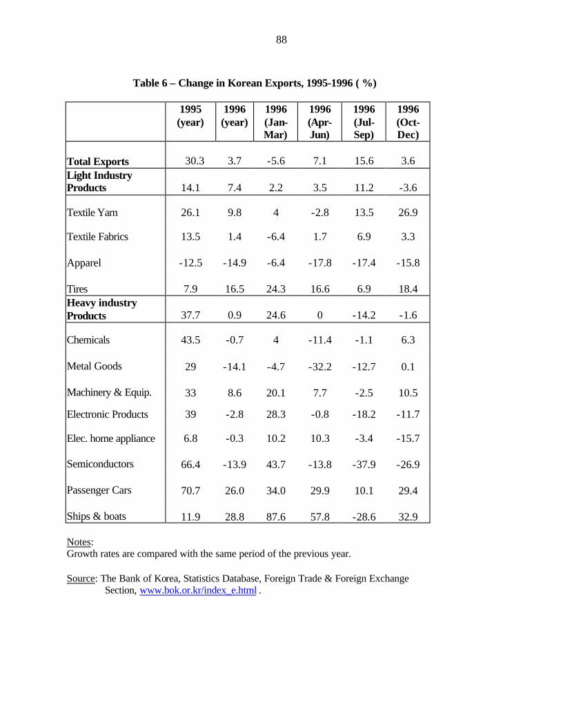
88

Table 6 – Change in Korean Exports, 1995-1996 ( %)

1995 (year)

1996 (year)

1996 (Jan-Mar)

1996 (Apr-Jun)

1996 (Jul-Sep)

1996 (Oct-Dec)

Total Exports 30.3 3.7 -5.6 7.1 15.6 3.6 Light Industry Products 14.1 7.4 2.2 3.5 11.2 -3.6

Textile Yarn 26.1 9.8 4 -2.8 13.5 26.9

Textile Fabrics 13.5 1.4 -6.4 1.7 6.9 3.3 Apparel -12.5 -14.9 -6.4 -17.8 -17.4 -15.8 Tires 7.9 16.5 24.3 16.6 6.9 18.4 Heavy industry Products 37.7 0.9 24.6 0 -14.2 -1.6

Chemicals 43.5 -0.7 4 -11.4 -1.1 6.3 Metal Goods 29 -14.1 -4.7 -32.2 -12.7 0.1 Machinery & Equip. 33 8.6 20.1 7.7 -2.5 10.5

Electronic Products 39 -2.8 28.3 -0.8 -18.2 -11.7

Elec. home appliance 6.8 -0.3 10.2 10.3 -3.4 -15.7 Semiconductors 66.4 -13.9 43.7 -13.8 -37.9 -26.9 Passenger Cars 70.7 26.0 34.0 29.9 10.1 29.4 Ships & boats 11.9 28.8 87.6 57.8 -28.6 32.9 Notes: Growth rates are compared with the same period of the previous year. Source: The Bank of Korea, Statistics Database, Foreign Trade & Foreign Exchange

Section, www.bok.or.kr/index_e.html .

89

Table 7. Bankruptcies in the Korean Chaebol, 1996-98

Name of Group Major Products Date Bankrupt Wooseong Construction 96-01-19 Hanbo Construction, steel 97-01-23 Sammi Steel 97-03-19 Jinro Liquor, foods 97-04-21 Hanshin Construction 97-05-31 Kia Auto Automobiles, steel 97-07-18 Dae-Nong Textiles, retail 97-09-11 Ssang-Bang-Ul Apparel, construction 97-10-20 Haitai Confectionary, beverages 97-11-03 Newcore Retail 97-11-04 Floating of the Korean won on November 17, 1997 Su-san Machinery 97-11-18 Tae-Il Hard disk drive 97-11-18 Sin-Ho Paper 97-11-28 Halla Auto parts, construction 97-12-08 Hanwha Explosives, chemicals 97-12-16 Jin-Do Fur coats, containers 97-12-16 Ssangyong Cement, construction 98-01-10 Dong-Ah Construction 98-01-10 Hanil Cement, construction 98-01-15 Nasan Textiles 98-01-15 Kukdong Construction 98-01-20 Kohap Textiles, plastics, chemicals 98-01-30 Chung-Gu Construction 98-04-23 Keopyung Chemicals, retailing 98-05-20

Source: Revised from Lee (1999). Notes: All firms belong to the top 60 largest conglomerates in terms of the asset values as of the end of 1996, assessed by the Bank Supervision Authority of Korea.

90

Table 8: Data for Top 30 Korean Chaebol, 1996-97

Business group

Sales ($million)

Debt/Equity 1996

Debt/Equity 1997

Short/Long debt, 1996

Short/Long debt, 1997

Prob. Of Bankruptcy

Hyundai 84,633 437 579 1.26 1.52 0.07 Samsung 70,194 270 367 0.96 0.92 0.00 LG 58,284 351 527 1.10 1.17 0.01 Daewoo 49,636 382 474 1.35 1.70 0.03 SK 28,195 350 461 2.01 2.01 0.01 Ssangyong 22,081 297 403 1.66 3.25 0.00 Kia 15,150 514 n.a. n.a. n.a. 0.19 Hanwha 11,405 665 1,066 1.58 3.09 0.61 Hanjin 10,810 558 920 0.43 0.26 0.30 Lotte 8,770 190 219 2.12 9.62 0.00 Hyosung 6,778 377 467 1.48 2.35 0.02 Daelim 5,976 418 508 1.42 2.16 0.05 Keumho 5,823 473 968 1.65 2.94 0.11 Kolong 4,989 341 421 1.63 0.03 0.01 Dong Ah 4,821 350 353 1.80 3.26 0.01 Halla 3,974 451 976 1.99 3.49 0.08 Doosan 3,919 743 623 1.80 4.98 0.78 Dongkuk Steel 3,817 219 323 1.10 1.21 0.00 Hanbo 3,549 675 1,501 n.a. n.a. 0.63 Haitai 3,227 521 814 1.70 3.09 0.21 Dongbu 3,227 250 350 1.74 3.67 0.00 Kohap 3,130 592 474 1.66 2.35 0.40 Hansol 2,979 340 459 1.35 0.87 0.01 Anam 2,427 526 1820 1.73 2.88 0.22 New Core 2,273 1224 1,784 n.a. n.a. 0.99 Dongyang 2,257 294 389 1.01 1.02 0.00 Sammi 1,856 -3,329 n.a. n.a. n.a. 1.00 Hanil 1,618 563 n.a. n.a. n.a. 0.31 Jinro 1,515 2,948 -813 1.45 2.44 1.00 Daesang 1,394 471 637 2.20 3.88 0.11 Shinho 1,224 391 798 1.28 1.64 0.03 Keopyung 1,053 269 357 1.57 2.60 0.00 Notes: 1. Groups shown in bold declared bankruptcy prior to November 17, 1997; groups in bold and italics declared bankruptcy after that date. 2. Group sales have been converted to US$ using the 1996 exchange rat of 804 won/$. 3. Debt/equity ratios and short term/long term loan ratios are at end of the calendar year, and exclude financial firms in each group. Sources: New Industry Management Academy (1999), supplemented with information from the Korean Fair Trade Commission.

91

Table 9: Regression results for Bankruptcy of Chaebol, 1996-98

Regression 1: Those chaebol going bankrupt before November 17, 1997

Probability of Bankruptcy = - 47 + 7.3 96Equity

96Debt ln , N=35, R2 =0.60

(s.e.= 3.4, p=0.03) No. of observations without bankruptcy = 27, Successfully predicted (probability < .5) = 26 No. of observations with bankruptcy = 8, Successfully predicted (probability > .5) = 6 Regressions 2: Those chaebol going bankrupt after November 17, 1997

(a) Pr(Bankrupt) = - 11 + 1.7 96Equity

96Debt ln , N=36, R2 =0.05

(s.e.=1.3, p=0.19) No. of observations without bankruptcy = 27, Successfully predicted (probability < .5) = 27 No. of observations with bankruptcy = 9, Successfully predicted (probability > .5) = 0

(b) Pr(Bankrupt) = - 1.8 + 0.12 97Equity

97Debt ln , N=27, R2 =0.00

(s.e.=0.97, p=0.70) No. of observations without bankruptcy = 20, Successfully predicted (probability < .5) = 20 No. of observations with bankruptcy = 7, Successfully predicted (probability > .5) = 0 (c) Excluding Doosan and Lotte groups from the estimation:

Pr(Bankrupt) = - 1.2 - 0.67 97Equity

97Debt ln + 2.7

97 loans termLong97 loans Short term

ln ,

(s.e.=1.1, p=0.55) (s.e.=1.5, p=0.06) N=25, R2 =0.22 No. of observations without bankruptcy = 18, Successfully predicted (probability < .4) = 15 No. of observations with bankruptcy = 7, Successfully predicted (probability > .4) = 4

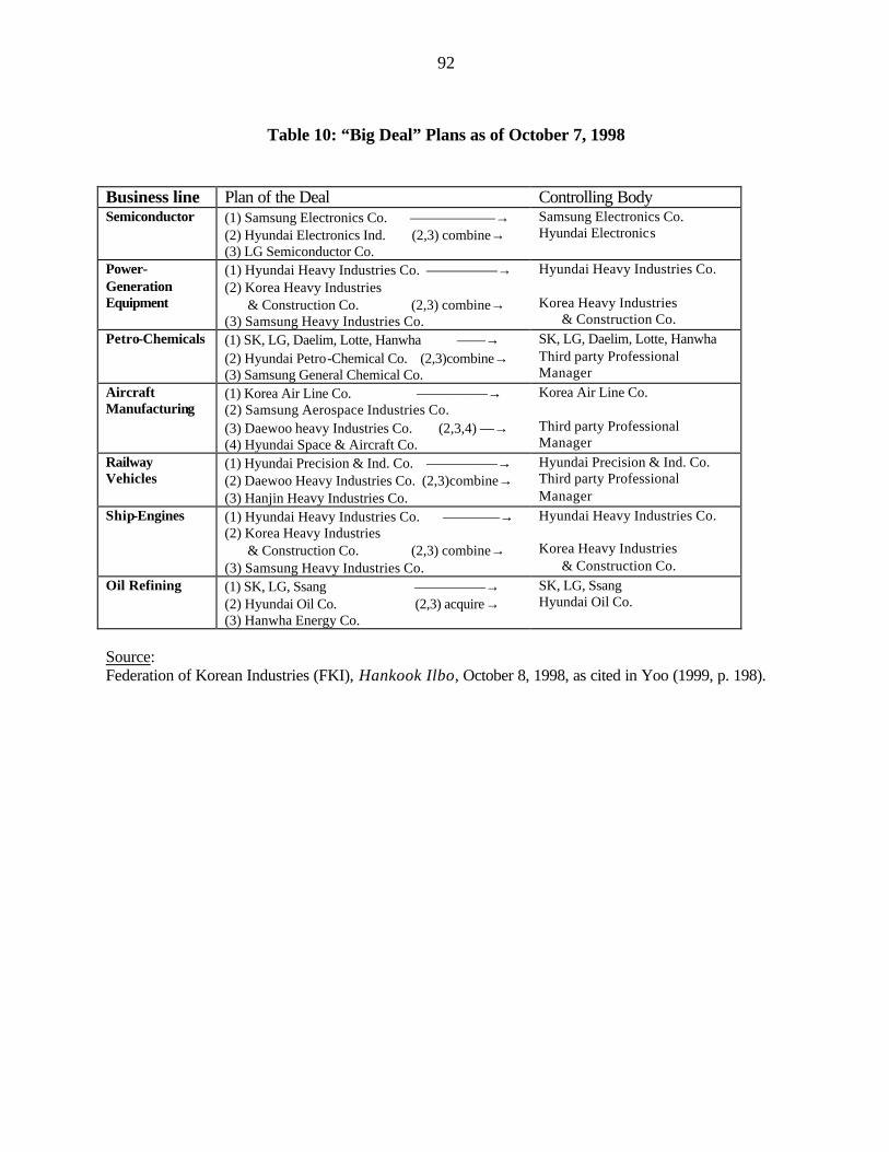
92

Table 10: “Big Deal” Plans as of October 7, 1998

Business line Plan of the Deal Controlling Body Semiconductor (1) Samsung Electronics Co. ——————→

(2) Hyundai Electronics Ind. (2,3) combine→ (3) LG Semiconductor Co.

Samsung Electronics Co. Hyundai Electronics

Power-Generation Equipment

(1) Hyundai Heavy Industries Co. —————→ (2) Korea Heavy Industries & Construction Co. (2,3) combine→ (3) Samsung Heavy Industries Co.

Hyundai Heavy Industries Co. Korea Heavy Industries & Construction Co.

Petro-Chemicals (1) SK, LG, Daelim, Lotte, Hanwha ——→ (2) Hyundai Petro-Chemical Co. (2,3)combine→ (3) Samsung General Chemical Co.

SK, LG, Daelim, Lotte, Hanwha Third party Professional Manager

Aircraft Manufacturing

(1) Korea Air Line Co. —————→ (2) Samsung Aerospace Industries Co. (3) Daewoo heavy Industries Co. (2,3,4) —→ (4) Hyundai Space & Aircraft Co.

Korea Air Line Co. Third party Professional Manager

Railway Vehicles

(1) Hyundai Precision & Ind. Co. —————→ (2) Daewoo Heavy Industries Co. (2,3)combine→ (3) Hanjin Heavy Industries Co.

Hyundai Precision & Ind. Co. Third party Professional Manager

Ship-Engines (1) Hyundai Heavy Industries Co. ————→ (2) Korea Heavy Industries & Construction Co. (2,3) combine→ (3) Samsung Heavy Industries Co.

Hyundai Heavy Industries Co. Korea Heavy Industries & Construction Co.

Oil Refining (1) SK, LG, Ssang —————→ (2) Hyundai Oil Co. (2,3) acquire→ (3) Hanwha Energy Co.

SK, LG, Ssang Hyundai Oil Co.

Source: Federation of Korean Industries (FKI), Hankook Ilbo, October 8, 1998, as cited in Yoo (1999, p. 198).

93

Upstream Sector:

Downstream Sector:

Group a Group b

Unaffiliated Firms

Unaffiliated Firms

Business Groups

Figure 1: Model of Business Groups

94

Group

Upstream Group (U-group):

Downstream Firms

Downstream Group (D-group):

Group

Upstream Firms

Vertically Integrated Groups (V-group):

Group a Group b

Figure 2: Types of Business Groups

95

Figure 3: Regions Where Groups Sell Inputs or Not

0

2

4

6

8

10

12

1 1.1 1.2 1.3 1.4 1.5 1.6 1.7 1.8 1.9 2

Elasticity of Substitution, S

Nu

mb

er o

f Gro

up

s, G

S=G/(G-1)

Groups sell inputsto each other

Groups do not sell inputs

Figure 4: Number of V-Groups

0

2

4

6

8

10

12

14

16

18

20

1 1.2 1.4 1.6 1.8 2 2.2 2.4 2.6 2.8 3 3.2 3.4

Elasticity of Substitution, S

Nu

mb

er o

f Gro

up

s, G

V-group (stable)

V-group (unstable)

S=G/(G-1)

96

Figure 5: Pricing of Inputs with V-groups

0

1

23

4

56

7

8

910

1.5 1.7 1.9 2.1 2.3 2.5 2.7 2.9 3.1 3.3 3.5

Elasticity of Substitution, S

Pri

ce o

f In

pu

t V-group(stable)

V-groups do not sell inputs externally

V-group(unstable)

Figure 6: Number of Business Groups

0

2

4

6

8

10

12

14

16

18

20

22

1 1.2 1.4 1.6 1.8 2 2.2 2.4 2.6 2.8 3 3.2 3.4

Elasticity of Substitution, S

Nu

mb

er o

f Gro

up

s, G

V-group (stable)

D-group

U-group

V-group (unstable)

?

S=G/(G-1)

97

Figure 7: Change in Korean Exports ($)

-15

0

15

30

45

1994

09

1994

12

1995

03

1995

06

1995

09

1995

12

1996

03

1996

06

1996

09

1996

12

1997

03

1997

06

1997

09

An

nu

al C

han

ge

(%)

Value of Exports Export Prices

Figure 8: Change in Export Prices to the U.S. ($)

-20

-15

-10

-5

0

5

1994

09

1994

12

1995

03

1995

06

1995

09

1995

12

1996

03

1996

06

1996

09

1996

12

1997

03

1997

06

1997

09

An

nu

al C

han

ge

(%

)

Korea Taiwan

98

Figure 9: Semiconductor Export Prices to the U.S. ($)

-50

-40

-30

-20

-10

0

10

1994

09

1994

12

1995

03

1995

06

1995

09

1995

12

1996

03

1996

06

1996

09

1996

12

1997

03

1997

06

1997

09

An

nu

al C

han

ge

(%

)

Korea Taiwan

Figure 10: V-Groups (Elasticity=3)

0

5

10

15

20

25

200 400 600 800 1000 1200 1400 1600

Demand, L

Nu

mb

er o

f Gro

up

s, G

A

B

C

Stable

(Unstable)

D

99

Figure 11: V-group Equilibria

0

500

1000

1500

Demand

2.5

2.75

3

3.25

3.5

Elasticity

0

10

20

G

0

500

1000

1500

Demand

0

10

20

G

100

Chaebol

Merchant Banks

Commercial Banks

Investment Projects

(long-term)

Foreign Funds

Short Term only

Top 5 Groups only

Loans (long term)

Loans –domestic & foreign currency

Deposits – long-term & short-term

Figure 12: Financial Structure in Korea

Commercial Paper (short-term)

Commercial Paper (short-term)

101

Appendix: Data on Business Groups

The primary source for the 1989 Korean data, shown in Table A1 is the volume 1990

Chaebol Analysis Report (Chaebol Boon Suk Bo Go Seo in Korean) published by Korea

Investors Service, Inc. Complete data were available for 44 groups, with 499 firms. The primary

sources for the 1994 Taiwan data are twofold: Business Groups in Taiwan, 1996/1997, published

by the China Credit Information Service (CCIS); and company annual reports to the Taiwan

stock exchange, for 1994, collected by the CCIS, and supplemented by interviews of selected

firms. Business Groups in Taiwan, 1996/1997, provides information on 115 business groups in

Taiwan. The 1994 database for Taiwan includes 80 groups, with 797 firms. These data are

described in detail in Feenstra (1997) and Feenstra, Hamilton and Huang (2001), from which the

summary Table A1 and A2 are drawn. Each table has the following information:

Column 1: Name of group

Column 2: Sales ($ million)

Column 3: Number of firms (* indicates that the group has a trading company)

Column 4: The internal sales ratio for each group, calculated as (internal sales within a

group)/(internal sales within a group plus all external sales to other firms or consumers).

Column 5: The internal sales ratio for each group, calculated by ignoring the purchases of trade

companies and other retail firms in a group. This internal sales ratio is calculated as (all internal

sales within a group, except those made to trading companies or other wholesale/retail firms)/(all

internal sales within a group, except those made to trading companies or other wholesale/retail

firms, plus all group sales to external firms or consumers).

102

Columns 6-7: The Herfindahl index, defined as ∑− i2is1 , where si is the share of total sales in

each sector i. To implement this index we divided the entire economy into 31 sectors, with 22 in

manufacturing and 7 in services. Each firm in a group is identified as selling in one of these

sectors by its major product category, and then the Herfindahl index is computed for each group.

We considered four different calculations: using all sales or just internal sales; and using all

products or just manufacturing. Column 6 reports the broadest case, where the Herfindahl index

is defined over all sales and all products; and column 7 the narrowest case, where the Herfindahl

index is defined over just manufacturing inputs sold internally to the group.

The averages shown at the bottom of each table are computed as simple average of the data in

each column, while the weighted averages use group sales as weights.

103

Table A1: Business Groups in Korea, 1989

Group Name 1989 Sales

($ mill.) Number of Firms (* TC)

Internal Sales

Ratio (%)

Internal Sales

(no Retail)

Herfindahl Index

(all sales)

Internal Sales

(internal manufact.)

Samsung 26,175 32* 31.9 18.8 0.70 0.35 Hyundai 25,500 30* 33.0 19.8 0.80 0.78 LG (Lucky Goldstar) 18,807 45* 26.0 12.5 0.74 0.46 Daewoo 13,837 24* 23.5 9.7 0.68 0.66 SK (Sunkyong) 8,910 16* 20.6 10.3 0.69 0.42 Ssangyong 5,777 15* 14.8 11.6 0.75 0.63 Hyosung 4,697 20* 7.4 3.3 0.20 0.04 Kia 4,602 9* 25.6 6.6 0.80 0.64 Lotte 3,900 23* 9.2 7.7 0.25 0.12 Han Jin 3,895 11* 2.7 2.2 0.63 0.43 Korea Explosives 3,172 19* 7.7 4.7 0.80 0.58 Doosan 2,417 17* 13.3 11.5 0.84 0.77 Kolon 2,218 14* 10.6 4.0 0.65 0.00 Dongbu 1,978 7* 26.1 17.3 0.50 0.12 Daelim 1,951 12* 4.4 0.6 0.38 0.27 Dongkuk Steel Mill 1,886 10* 5.4 3.4 0.27 0.01 Dong Ah Construction 1,866 12* 1.1 0.7 0.39 0.00 Sammi 1,696 5* 36.6 27.0 0.51 0.00 Kumho 1,430 8* 3.3 0.4 0.64 0.00 Hanil 1,296 12* 7.1 7.1 0.61 0.39 Miwon 1,295 13* 12.5 6.4 0.65 0.26 Halla 1,262 7 10.2 10.2 0.62 0.51 Kangwon Industries 1,256 12* 33.5 11.4 0.74 0.31 Samyang 1,038 5 1.6 1.6 0.41 0.63 Kohap 1,016 6* 18.2 12.5 0.53 0.37 Poongsan 941 6 3.3 3.3 0.36 0.08 Woosung Construction 834 6 2.0 2.0 0.47 0.00 Kukdong Oil 812 3 19.3 0.0 0.39 0.00 Dongkuk Corporation 689 7* 11.3 1.1 0.55 0.00 Tongil 685 10 4.4 4.4 0.74 0.08 Tong Yang 672 5* 9.3 9.3 0.49 0.33 Byucksan 661 17 0.6 0.6 0.75 0.50 Taejon Leather 627 7 1.6 1.6 0.61 0.11 Daesung Industries 589 8 2.0 2.0 0.55 0.55 Anam Industrial 537 5 8.7 8.7 0.28 0.00 Oriental Chemical 528 9 8.9 8.9 0.40 0.48 Jinro 490 40 2.6 2.6 0.63 0.14 Taihan Electric Wire 490 3 3.0 3.0 0.12 0.00 Kyesung Paper 437 5 17.3 17.3 0.28 0.00 Han Yang 436 4* 6.6 0.7 0.22 0.00 Hanbo 420 3 2.6 2.6 0.35 0.44 You One Construction 281 2* 0.3 0.0 0.41 0.00 Kuk Dong Construction 247 4 0.1 0.1 0.10 0.00 Life Construction 211 4 3.5 3.5 0.48 0.00

Average 3,441 11.3 11.3 6.7 0.52 0.26 Weighted Average 23.9 22.1 12.2 0.66 0.45

104

Table A2: Business Groups in Taiwan, 1994

Group Name 1994 Sales

($ mill.) Number of Firms (* TC)

Internal Sales

Ratio (%)

Internal Sales

(no Retail)

Herfindahl Index

(all sales)

Internal Sales

(internal manufact.)

Formosa Plastics 6,654 16 15.8 15.8 0.54 0.58 Shin Kong 5,724 25* 0.4 0.4 0.40 0.22 Wei Chuan Ho Tai 4,889 23* 28.1 0.4 0.55 0.02 Far Eastern 4,291 26 0.7 0.5 0.53 0.05 Yulon 4,264 23* 26.6 5.2 0.77 0.26 President 3,932 31* 6.4 4.5 0.70 0.29 Tatung 3,634 36 8.3 6.3 0.38 0.18 Acer 3,243 9* 3.5 2.4 0.62 0.01 Chinfon 2,986 16* 24.1 1.1 0.19 0.00 Hualon 2,517 9* 16.4 4.7 0.70 0.00 Ho Hsin 2,104 15* 0.2 0.2 0.50 Tuntex 1,831 16* 8.1 7.9 0.78 0.38 Teco Electric & Machinery 1,474 17* 2.6 2.6 0.60 0.15 Chi Mei 1,268 6* 0.3 0.3 0.25 0.09 Rebar 1,221 9* 1.4 0.9 0.72 0.00 Pacific Cable 1,214 26 3.2 3.2 0.54 0.05 Sampo 1,096 11 12.5 12.5 0.26 0.00 Tainan Spining 1,075 17 2.1 2.1 0.71 0.00 Pacific Construction 1,032 15 2.8 2.7 0.63 0.46 Yuen Foong Yu 1,000 8* 18.5 4.5 0.46 0.13 Ruentex 997 25* 0.7 0.0 0.51 0.00 Taiwan Cement 997 16 3.6 3.6 0.48 0.39 Lien Hwa Mitac 900 12* 2.8 2.7 0.53 0.00 Walsin Lihwa 881 8 0.1 0.1 0.02 0.06 Lite-On 875 10 0.5 0.5 0.71 0.50 Kwang Yang 855 7* 6.3 6.3 0.20 0.18 Cheng Loong 823 7* 16.3 16.2 0.08 0.00 Shih Lin Paper 766 5 0.1 0.1 0.20 0.00 United Microelectronics 673 4 8.5 8.5 0.00 0.00 Chung Shing Textile 668 5 6.6 6.1 0.50 0.00 Yeang Der 618 14 1.0 0.1 0.37 0.02 China General Plastics 598 5 12.6 12.6 0.67 0.00 Chun Yuan Steel 528 5 4.7 4.7 0.36 0.00 Adi 484 9 0.7 0.3 0.22 0.00 Shinlee 456 12* 0.4 0.4 0.52 0.00 Umax Elitegroup 436 8* 7.2 7.2 0.00 0.00 Pou Chen Industrial 434 3 4.5 4.5 0.49 0.50 Aurora 406 7* 17.5 8.6 0.09 0.00 Ase 404 5* 10.5 1.3 0.35 0.00 Great Wall 375 12 21.1 20.7 0.31 0.17

105

Ho Cheng 375 8* 14.5 14.5 0.26 0.00 Taiwan Glass 350 9* 2.6 0.6 0.00 0.00 Tung Ho Steel 350 4 0.6 0.6 0.25 0.09 Lealea 335 7 9.4 9.4 0.17 0.00 Vedan 327 8* 8.1 7.5 0.04 0.00 Chia Hsin Cement 303 7* 7.0 7.0 0.00 0.00 Hwa Eng Cable 303 3 8.9 8.9 0.51 0.00 Lily Textile 301 7 0.7 0.7 0.04 0.00 Chia Her 293 5 1.6 1.6 0.38 0.00 Sun Moon Star 287 5* 7.1 3.8 0.49 0.00 Ta Ya Cable 276 6 4.0 4.0 0.10 0.21 Shing Nung 256 13* 6.2 5.9 0.42 0.22 Tah Tong Textile 235 13* 4.5 0.7 0.55 0.39 Dahin 231 5* 12.3 9.9 0.51 0.21 Chicony Electronics 217 3 4.3 4.3 0.00 0.00 Kenda Industrial 211 8 0.5 0.5 0.49 0.00 Lee Tah Farm Industrial 204 5 11.6 11.6 0.19 0.50 Fwu Sow Industrial 200 7* 7.1 7.0 0.01 0.00 Asia Chemical 180 13* 4.6 2.7 0.10 0.00 Men Yi 170 4 1.0 1.0 0.00 0.00 China Unique 166 4 2.8 2.8 0.22 0.00 Ve Wong 161 3 10.0 10.0 0.00 0.00 Hong Ho Precision Textile 159 6* 3.4 3.4 0.10 0.00 Chun Yu 158 7* 6.1 5.3 0.45 0.50 Ability 157 11 2.2 2.2 0.26 0.38 Far Eastern Machinery 156 7 0.3 0.3 0.20 0.00 UB 139 8 7.4 7.4 0.48 0.00 Chien Shing Stainless Steel 137 6 8.4 8.4 0.17 0.00 South East Cement 134 5 8.0 8.0 0.12 0.46 Bomy 116 9 29.5 0.0 0.48 0.00 Taiwan Everlight Chemical 104 5* 14.2 3.5 0.30 0.00 Ching Kuang Chemical 104 3 10.6 10.6 0.26 0.00 Nan Pao Resins 104 3 8.4 8.4 0.22 0.00 Victor Machinery 101 12* 1.2 1.2 0.16 0.00 Ren Hou (Chih Lien) 83 10* 0.0 0.0 0.51 0.00 Yung Shin Pharmaceutical 78 8* 2.7 1.8 0.05 0.00 Fu I Industrial 77 5* 5.1 5.1 0.30 0.00 San Wu Textile 53 3 2.7 2.7 0.57 0.05 Fong Kuo 48 4 6.5 6.5 0.34 0.10 Tong Hsing 35 4* 2.8 2.0 0.57 0.00

Average 954 10.0 7.0 4.7 0.35 0.10 Weighted Average 16.9 9.5 4.5 0.48 0.16