(ch.6. two-level factorial...

Hae-Jin ChoiSchool of Mechanical Engineering,

Chung-Ang University

4. The 2k Factorial Designs

(Ch.6. Two-Level Factorial Designs)

1DOE and Optimization

Introduction to 2k Factorial Designs

Special case of the general factorial design; k factors, all at two levels

The two levels are usually called low and high (they could be either quantitative or qualitative)

Very widely used in industrial experimentation

Form a basic “building block” for other very useful experimental designs

Useful for factor screening


Chemical Process Example

A = reactant concentration, B = catalyst amount, y =

recovery


The Simplest Case: The 22

“-” and “+” denote the low and high

levels of a factor, respectively

Low and high are arbitrary terms

Geometrically, the four runs form

the corners of a square

Factors can be quantitative or

qualitative, although their

treatment in the final model will

be different


Notation of the 2k Designs

DOE and Optimization 5

A special notation is used to represent the runs. In general, a run is

represented by a series of lower case letters. If a letter is present,

then the corresponding factor is set at the high level in that run; if it

is absent, the factor is run at its low level. For example, run a

indicates that factor A is at the high level and factor B is at the low

level. The run with both factors at the low level is represented by

(1).

This notation is used throughout the 2k design series. For example,

the run in a 24 with A and C at the high level and B and D at the low

level is denoted by ac.

Estimation of Factor Effects

12

12

12

(1)

2 2

[ (1)]

(1)

2 2

[ (1)]

(1)

2 2

[ (1) ]

A A

n

B B

n

n

A y y

ab a b

n n

ab a b

B y y

ab b a

n n

ab b a

ab a bAB

n n

ab a b

The letters (1), a, b, and ab also

represent the totals of all n

observations taken at these

design points.

6DOE and OptimizationOrthogonal Design

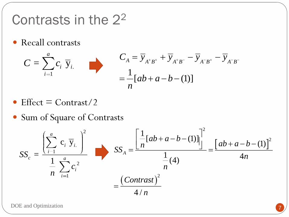
Contrasts in the 22

Recall contrasts

Effect = Contrast/2

Sum of Square of Contrasts

.

1

= ya

i i

i

C c

2

.

1

2

1

c y

= 1

a

i i

i

c a

i

i

SS

cn

1[ (1)]

A A B A B A B A BC y y y y

ab a bn

2

2

2

1[ (1)]

(1)

1 4(4)

4 /

A

ab a bab a bn

SSn

n

Contrast

n


Sum of Squares of the 22 Designs

The analysis of variance is

completed by computing

the total sum of squares

SST (with 4n-1 degrees of

freedom) as usual, and

obtaining the error sum of

squares SSE [with 4(n-1)

degrees of freedom] by

subtraction.

SSa ab b

n

SSb ab a

n

SSab a b

n

A

B

AB

[ ( )]

[ ( )]

[ ( ) ]

1

4

1

4

1

4

2

2

2


ANOVA of the Chemical Processing

The F-test for the “model” source is testing the significance of the

overall model; that is, is either A, B, or AB or some combination of

these effects important?


Regression Model


Regression model for 2k Designs

Where x1 is coded variable of Factor A and x2 is coded variable

of Factor B

Low lever = -1 and High level = +1

Relationship between natural and coded variables

1 1 2 2 3 1 2oy x x x x

1

( ) / 2

/ 2

A A Ax

A A

Regression Model for Chemical Processing


Since interaction effect is very small, the regression model

employed is

where x1 is coded variable of the reactant concentration and x2 is

coded variable of the amount of catalyst

1 1 2 2oy x x

1

( ) / 2

/ 2

(25 15) / 2 20

(25 15) / 2 5

high low

high low

Conc Conc Concx

Conc Conc

Conc Conc

2

1.5

0.5

Catalystx

Regression Model for Chemical Processing


Estimating of the regression model, using least square

method We will return to least square method in response surface method

Regression model with coded factors is

where 27.5 is grand average of all observation, is one-half of the

corresponding factor effect estimates

Regression model with uncoded factors

0 1 2, ,

1 2

8.33 5.00ˆ 27.5

2 2y x x

8.33 20 5.00 1.5ˆ 27.5

2 5 2 0.5

18.33 0.8333 5.00

Conc Catalysty

Conc Catalyst

1 2ˆ ˆ,

Residual Analysis of Chemical Processing


Residual

For example

ˆy y

1 28 25.8358.33 5.00

ˆ 27.5 ( 1) ( 1)2 2

y

Review of Analysis Procedure

Estimate factor effects Main effects, interaction effects

Formulate model 22 design example

Statistical testing (ANOVA)

Refine the model Chemical processing example

Regression model estimation By Least Square Method

Analyze residuals (graphical) Normal probability plot of residuals

Interpret results

1 1 2 2 3 1 2oy x x x x

1 1 2 2oy x x

1 1 2 2ˆ ˆ ˆˆ

oy x x


The 23 Factorial Design


Factor Effect of the 23 Designs


3 factors, each at two levels

8 factor-level combinations

3 main effects: A,B,C

3 two-factor interactions:

AB, AC,BC

1 three-factor interaction:

ABC



Main effect of A

Main effect of B

Main effect of C

1(1)

4A a ab ac abc b c bc

n

1(1)

4B b ab bc abc a c ac

n

1(1)

4C c ac bc abc a b ab

n



Interaction effect of AB

The same approach can be applied for the interaction effect of BC

and AC

1( ) ( )

2

1 1( ) [ (1)] [ ]

2 2

1 1( ) [ ] [ ]

2 2

1[ (1) ]

4

high low

low

high

AB AB C AB C

where

AB C ab a bn n

AB C abc c ac bcn n

Therefore

AB ab abc c b a bc acn



Interaction effect of ABC is defined as the average difference

between the AB interaction at the two different level of C

How to memorize the sign of coefficients?

1( ) ( )

2

1 1 1 1 1 ) ( ) - (1)

2 2 2 2n 2

1 - - + - + + -(1)

4

ABC AB C high AB C low

abc c ac ab ab a bn n n

abc bc ac c ab b an

Properties of the Table

Except for column I, every column has an equal number of + and – signs

The sum of the product of signs in any two columns is zero

Multiplying any column by I leaves that column unchanged (identity element)

The product of any two columns yields a column in the table:

Orthogonal design

Orthogonality is an important property shared by all factorial designs

2

A B AB

AB BC AB C AC


Effects, Sum of Squares, and Contrast


The 23 Designs

Effect = Contrast/4

Sum of squares = n(Contrast)2/8

Contrast for factor A

Main effect of factor A

Sum of Square of factor A

1(1)AContrast a ab ac abc b c bc

n

1/ 4 (1)

4AA Contrast a ab ac abc b c bc

n

22 1( ) / 8 (1)

8A ASS n Contrast a ab ac abc b c bc

n

Plasma Etching Process

A 23 factorial design was used to

develop a nitride etch process on a

single-wafer plasma etching tool. The

design factors are the gap between the

electrodes, the gas flow (C2F6 is used

as the reactant gas), and the RF power

applied to the cathode. Each factor is

run at two levels, and the design is

replicated twice. The response variable

is the etch rate for silicon nitride

(Å/m)

A = gap, B = Flow, C = Power, y = Etch Rate


Plasma Etching Process


Plasma Etching

ProcessWafer

Gap Gas flow Power

Etch rate

ANOVA Summary – Full Model

Important effects by A, C, AC,


The Regression Model with Reduced Factors


Cube Plot of Ranges

What do the large

ranges when gap

and power are at

the high level tell

you?


The General 2k Factorial Design


1

2

2

( )

2

k

k

ContrastEffect

n ContrastSS

Unreplicated 2k Factorial Designs

These are 2k factorial designs with one observation at each corner of the “cube”

An unreplicated 2k factorial design is also sometimes called a “single replicate” of the 2k

These designs are very widely used

Risks…if there is only one observation at each corner, is there a chance of unusual response observations spoiling the results?


Spacing of Factor Levels in the Unreplicated 2k

Factorial Designs

If the factors are spaced too closely, it increases the chances that the noise will

overwhelm the signal in the data

More aggressive spacing is usually best


Unreplicated 2k Factorial Designs

Lack of replication causes potential problems in statistical testing Replication admits an estimate of “pure error” (a better phrase is an

internal estimate of error)

With no replication, fitting the full model results in zero degrees of freedom for error

Potential solutions to this problem Pooling high-order interactions to estimate error

Normal probability plotting of effects (Daniels, 1959)


Example of an Unreplicated 2k Design

A chemical product is produced in a pressure vessel. A factorial

experiment is carried out in the pilot plant to study the factors

thought to influence the filtration rate of this product .

The factors are A = temperature, B = pressure, C = mole ratio, D=

stirring rate

A 24 factorial was used to investigate the effects of four factors on

the filtration rate of a resin

Experiment was performed in a pilot plant


The Resin Plant Experiment


Contrast Constants for the 24 Design


Estimates of the Effects


ANOVA Summary for the Model as a 23 in Factors A, C,

and D


The Regression Model


Experiments with the larger number of factors

The system is usually dominated by the main effects and low-order interactions. Higher interactions are usually negligible.

When the number of factors is larger than 3 or 4, a common practice is to run only a single replicate design and then pool the higher order interactions as an estimate of error.

Normal probability plot of the effects may be useful

If none of the effects is significant, then the estimates will behave like a random sample drawn from a normal distribution with zero mean, and the plotted effects will lie approximately along a straight line.

Those effects that do not plot on the line are significant factors.


(ch.6. two-level factorial...

Documents