ch2 - whitman people

“ch2”2003/8/page 1

C H A P T E R 2

Qualitative Modeling withFunctions

It is often surprising that very simple mathematical modeling ideas can produceresults with added value. Indeed, the solutions may be elegant and provide qualityof understanding that obviates further exploration by more technical or complexmeans. In this chapter we explore a few simple approaches to qualitatively modelingphenomena with well-behaved functions.

2.1 MODELING SPECIES PROPAGATION

This problem concerns the factors that influence the number of species existing onan island. The discussion is adapted from [1].

One might speculate that factors affecting the number of species could include

• Distance of the island from the mainland

• Size of the island

Of course limiting ourselves to these influences has the dual effect of making atractable model that needs to be recognized as omitting many possible factors.

The number of species may increase due to new species discovering the islandas a suitable habitat. We will refer to this as the migration rate. Alternatively,species may become extinct due to competition. We will refer to this as the ex-tinction rate. This discussion will be simplified by employing an aggregate total forthe number of species and not attempting to distinguish the nature of each species,i.e., birds versus plants.

Now we propose some basic modeling assumptions that appear reasonable.

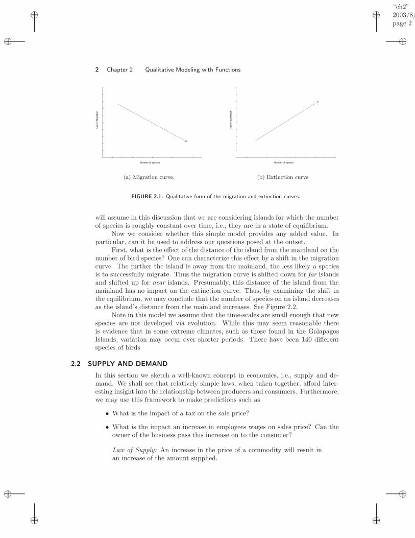
The migration rate of new species decreases as the number of species onthe island increases.

The argument for this is straight forward. The more species on an island the smallerthe number of new species there is to migrate. See Figure 2.1 (a) for a qualitativepicture.

The extinction rate of species increases as the number of species on theisland increases.

Clearly the more species there are the more possibilities there are for species to dieout. See Figure 2.1 (b) for a qualitative picture.

If we plot the extinction rate and the migration rate on a single plot weidentify the point of intersection as an equilibrium, i.e., the migration is exactlyoffset by the extinction and the number of species on the island is a constant. We

1

“ch2”2003/8/page 2

2 Chapter 2 Qualitative Modeling with Functions

Number of species

Rat

e of

Mig

ratio

n

M

(a) Migration curve.

Number of species

Rat

e of

Ext

inct

ion

E

(b) Extinction curve

FIGURE 2.1: Qualitative form of the migration and extinction curves.

will assume in this discussion that we are considering islands for which the numberof species is roughly constant over time, i.e., they are in a state of equilibrium.

Now we consider whether this simple model provides any added value. Inparticular, can it be used to address our questions posed at the outset.

First, what is the effect of the distance of the island from the mainland on thenumber of bird species? One can characterize this effect by a shift in the migrationcurve. The further the island is away from the mainland, the less likely a speciesis to successfully migrate. Thus the migration curve is shifted down for far islandsand shifted up for near islands. Presumably, this distance of the island from themainland has no impact on the extinction curve. Thus, by examining the shift inthe equilibrium, we may conclude that the number of species on an island decreasesas the island’s distance from the mainland increases. See Figure 2.2.

Note in this model we assume that the time-scales are small enough that newspecies are not developed via evolution. While this may seem reasonable thereis evidence that in some extreme climates, such as those found in the GalapagosIslands, variation may occur over shorter periods. There have been 140 differentspecies of birds

2.2 SUPPLY AND DEMAND

In this section we sketch a well-known concept in economics, i.e., supply and de-mand. We shall see that relatively simple laws, when taken together, afford inter-esting insight into the relationship between producers and consumers. Furthermore,we may use this framework to make predictions such as

• What is the impact of a tax on the sale price?

• What is the impact an increase in employees wages on sales price? Can theowner of the business pass this increase on to the consumer?

Law of Supply: An increase in the price of a commodity will result inan increase of the amount supplied.

“ch2”2003/8/page 3

Section 2.2 Supply and Demand 3

Number of species

E

M

Near Island

Far Island

FIGURE 2.2: The effect of distance of the island from the mainland is to shift the migration curve.Consequently the equilibrium solution dictates a smaller number of species will be supported for islandsthat are farther away from the mainland.

Law of Demand: If the price of a commodity increases, then the quantitydemanded will decrease.

Thus, we may model the supply curve qualitatively by a monotonically in-creasing function. For simplicity we may assume a straight line with positive slope.Analogously, we may model the demand curve qualitatively by a monotonicallydecreasing function, which again we will take as a straight line.

A flat demand curve may be interpreted as consumers being very sensitive tothe price of a commodity. If the price goes up just a little, then the quantity indemand goes down significantly. Steep and flat supply and demand curves all havesimilar qualitative interpretations (see the problems).

2.2.1 Market Equilibrium

Given a supply curve and a demand curve we may plot them on the same axisand note their point of intersection (q∗, p∗). This point is special for the followingreason:

• The seller is willing to supply q∗ at the price p∗

• The demand is at the price p∗ is q∗

So both the supplier(s) and the purchaser(s) are happy economically speaking.

“ch2”2003/8/page 4


Supply Curve

Quantity

Pric

e

(a) Supply curve

Demand Curve

Quantity

Pric

e

(b) Demand curve

FIGURE 2.3: (a) Qualitative form of supply and demand curves.

“ch2”2003/8/page 5

Section 2.2 Supply and Demand 5

0 0.1 0.2 0.3 0.4 0.5 0.6 0.7 0.8 0.9 10

0.1

0.2

0.3

0.4

0.5

0.6

0.7

0.8

0.9

1

(q1,p

1)(q

2,p

1)

(q2,p

2)

(q3,p

2)

D

S

o o

o o

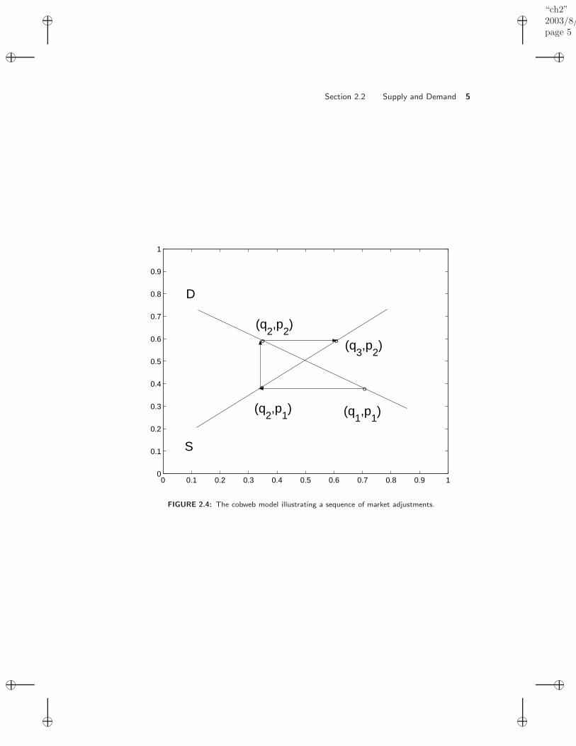
FIGURE 2.4: The cobweb model illustrating a sequence of market adjustments.

“ch2”2003/8/page 6


2.2.2 Market Adjustment

Of course, in general markets do not exist in the perfect economic utopia describedabove. We may model the market adjustment as a sequence of points on the demandand supply curves.

Based on market research it is estimated that consumers will demand a quan-tity q1 at a price p1. The supply and demand curves will permit a prediction ofhow the market will evolve. For simplicity, we will assume that the initial point(q1, p1) is on the demand curve to the right of the equilibrium point.

At the price p1 the supplier looks to his supply curve and proposes to sell areduced quantity q2. Thus we move from right to left horizontally. Note that movingvertically to the supply curve would not make sense as this would correspond tooffering the quantity q1 at an increased price. These goods will not sell at this price.

From the point (q1, p2) the consumer will respond to the new reduced quantityq2 by being willing to pay more. This corresponds to moving vertically upward tothe new point (q2, p2) on the supply curve.

Now the supplier adjusts to the higher price being paid in the market placeby increasing the quantity produced to q3. This process then continues, in theory,until an equilibrium is reached. It is possible that this will never happen, at leastnot without a basic adjustment to the shape of either the supply of demand curves,for example through cost cutting methods such as improved efficiency, or layoffs.

2.2.3 Taxation

The effect of a new tax on a product is to shift the demand curve down becauseconsumers will not be willing to pay as much for the product (before the tax).Note that this leads to a new equilibrium point which reduces the price paid tothe seller per item and reduces the quantity supplied by the producer. Thus onemay conclude from this picture that the effect of a tax on alcohol is to reduceconsumption as well as profit for the supplier. See Figure 2.5.

2.3 MODELING WITH PROPORTION AND SCALE

In the previous sections we have considered how simple functions may be employedto qualitatively model various situations and produce added value. Now we turn toconsiderations that assist in determining the nature of these functional dependenciesin more complex terms.

2.3.1 Proportion

If a quantity y is proportional to a quantity x then we write

y ∝ x

by which is meant

y = kx

for some constant of proportionality k.

“ch2”2003/8/page 7

Section 2.3 Modeling with Proportion and Scale 7

Quantity (q)

Pric

e (p

)

D before tax

S

D after tax

(qold

,pold

)

(qnew

,pnew

)

Shift (amount of tax)

Cost burden to supplier

Cost burdento consumer

New cost to consumer

FIGURE 2.5: A tax corresponds to a downwards shift in the demand curve.

“ch2”2003/8/page 8


EXAMPLE 2.1

In 1678 Robert Hooke proposed that the restoring force F of a spring is proportionalto its elongation e, i.e.,

F ∝ e

or,F = ke

where k is the stiffness of the spring.

Note that the property of proportionality is symmetric, i.e.,

y ∝ x → x ∝ y (2.1)

and transitive, i.e.,y ∝ x and z ∝ y → z ∝ x (2.2)

EXAMPLE 2.2

If y = kx + b where k, b are constants, then

y 6∝ x

buty − b ∝ x

Inverse proportion. If y ∝ 1/x then y is said to be inversely proportional tox.

EXAMPLE 2.3

If y varies inversely as the square-root of x then

y =k√x

Joint Variation. The volume of a cylinder is given by

V = πr2h

where r is the radius and h is the height. The volume is said to vary jointly withr2 and h, i.e.,

V ∝ r2 and V ∝ h

“ch2”2003/8/page 9


EXAMPLE 2.4

The volume of a given mass of gas is proportional to the temperature and inverselyproportional to the pressure, i.e., V ∝ T and V ∝ 1/P , or,

V = kT

P

EXAMPLE 2.5

Frictional drag due to the atmosphere is jointly proportional to the surface area Sand the velocity v of the object.

Superposition of Proportions. Often a quantity will vary as the sum of pro-portions.

EXAMPLE 2.6

The stopping distance of a car when an emergency situation is encountered is thesum of the reaction time of the driver and the amount of time it takes for the breaksto dissipate the energy of the vehicle. The reaction distance is proportional to thevelocity. The distance travelled once the breaks have been hit is proportional tothe velocity squared. Thus,

stopping distance = k1v + k2v2

EXAMPLE 2.7

Numerical error in the computer estimation of the center difference formula for thederivative is given by

e(h) =c1

h+ c2h

2

where the first term is due to roundoff error (finite precision) and the second termis due to truncation error. The value h is the distance δx in the definition of thederivative.

Direct Proportion. Ify ∝ x

we say y varies in direct proportion to x. This is not true, for example, if y ∝r2. On the other hand, we may construct a direct proportion via the obviouschange of variable x = r2. This simple trick always permits the investigation of therelationship between two variables such as this to be recast as a direct proportion.

“ch2”2003/8/page 10


−2 −1.5 −1 −0.5 0 0.5 1 1.5 20

0.2

0.4

0.6

0.8

1

1.2

1.4

1.6

1.8

2

y =

r2 /2

r

(a) Plot of y against r for y = r2/2.

0 0.5 1 1.5 2 2.5 3 3.5 40

0.2

0.4

0.6

0.8

1

1.2

1.4

1.6

1.8

2

r2y

= r

2 /2

Slope 1/2

(b) Plot of y = r2/2 against r2.

−2 −1.5 −1 −0.5 0 0.5 1 1.5 2−1

0

1

2

3

4

5

6

y =

kr(

r−1)

r

(c) Plot of y against r for y = kr(r+1).

−1 0 1 2 3 4 5 6−1

0

1

2

3

4

5

6

r(r−1)

y =

kr(

r−1)

slope k

(d) Plot of y = kr(r+1) againstr(r+1)

FIGURE 2.6: Simple examples of how a proportion may be converted to a direct proportion.

“ch2”2003/8/page 11


2.3.2 Scale

Now we explore how the size of an object can be represented by an appropriatelength scale if we restrict our attention to replicas that are geometrically similar.For example, a rectangle with sides l1 and w1 is geometrically similar to a rectanglewith sides l2 and w2 if

l1l2

=w1

w2= k (2.3)

As the ratio κ = l1/w1 characterizes the geometry of the rectangle it is referredto as the shape factor. If two objects are geometrically similar, then it can beshown that they have the same shape factor. This follows directly from multiplyingEquation (2.3) by the factor l2/w1, i.e.,

l1w1

=l2w2

= kl2w1

Characteristic Length.Characteristic length is useful concept for characterizing a family of geomet-

rically similar objects. We demonstrate this with an example.Consider the area of a rectangle of side l and width w where l and w may

vary under the restriction that the resulting rectangle be geometrically similar tothe rectangle with length l1 and width w1. An expression for the area of the varyingtriangle can be simplified as a consequence of the constraint imposed by geometricsimilarity. To see this

A = lw

= l(w1l

l1)

= κl2

where κ = w1/l1, i.e., the shape factor. See Figure 2.7 for examples of characteristiclengths for the rectangle.

EXAMPLE 2.8

Watering a farmer’s rectangular field requires an amount of area proportional tothe area of the field. If the characteristic length of the field is doubled, how muchadditional water q will be needed, assuming the new field is geometrically similarto the old field? Solution: q ∝ l2, i.e., q = kl2. Hence

q1 = kl21

q2 = kl22

Taking the ratio producesq1

q2=

l21l22

“ch2”2003/8/page 12


h

w

d

FIGURE 2.7: The height l1, the width l2 and the diagonal l3 are all characteristic lengths for therectangle.

Now if q2 = 100 acre feet of water are sufficient for a field of length l2 = 100, howmuch water will be required for a field of length l1 = 200? Sol.

q1 = q2l21l22

= 1002002

1002= 400 acre feet �

EXAMPLE 2.9

Why are gymnasts typically short? It seems plausible that the ability A, or naturaltalent, of gymnast would be proportional to strength and inversely proportional toweight, i.e.,

A ∝ strength

and

A ∝ 1weight

and taken jointly

A ∝ strengthweight

One model for strength is that the strength of a limb is proportional to the cross-sectional area of the muscle. The weight is proportional to the volume (assumingconstant density of the gynmast). Now, assuming all gymnasts are geometricallysimilar with characteristic length l

strength ∝ muscle area ∝ l2

“ch2”2003/8/page 13


andweight ∝ volume ∝ l3

so the ability A follows

A ∝ l2

l3∝ 1

l

So shortness equates to a talent for gymnastics. This problem was originally intro-duced in [2]. �

EXAMPLE 2.10

Proportions and terminal velocity. Consider a uniform density spherical objectfalling under the influence of gravity. The object will travel will constant (terminal)velocity if the accelerating force due to gravity Fg = mg is balance exactly by thedecelerating force due to atmospheric friction Fd = kSv2; S is the cross-sectionalsurface area and v is the velocity of the falling object. Our equilibrium conditionis then

Fg = Fd

Since surface area satisfies S ∝ l2 it follows l ∝ S1/2. Given uniform densitym ∝ w ∝ l3 so it follows l ∝ m1/3. Combining proportionalities

m1/3 ∝ S1/2

from which it follows by substitution into the force equation that

m ∝ m2/3v2

or, after simplifying,v ∝ m1/6

�

EXAMPLE 2.11

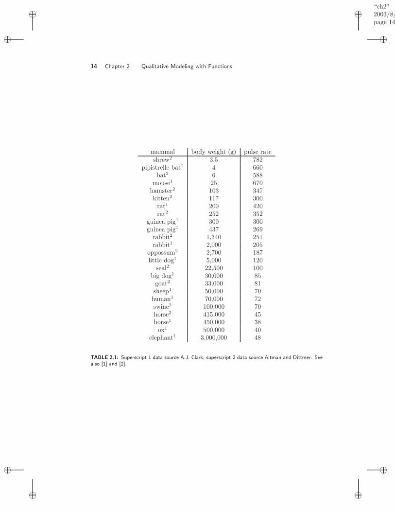
In this example we will attempt to model observed data displayed in Table 2.1 thatrelates the heart rate of mammals to there body weight. From the table we seethat we would like to relate the heart rate as a function of body weight. Smalleranimals have a faster heart rate than larger ones. But how do we estimate thisproportionality?

We begin by assuming that all the energy E produced by the body is usedto maintain heat loss to the environment. This heat loss is in turn proportional tothe surface area s of the body. Thus,

E ∝ s

The energy available to the body is produced by the process of respiration and isassumed to be proportional to the oxygen available which is in turn proportional

“ch2”2003/8/page 14


mammal body weight (g) pulse rateshrew2 3.5 782

pipistrelle bat1 4 660bat2 6 588

mouse1 25 670hamster2 103 347kitten2 117 300rat1 200 420rat2 252 352

guinea pig1 300 300guinea pig1 437 269

rabbit2 1,340 251rabbit1 2,000 205

oppossum2 2,700 187little dog1 5,000 120

seal2 22,500 100big dog1 30,000 85goat2 33,000 81sheep1 50,000 70human1 70,000 72swine2 100,000 70horse2 415,000 45horse1 450,000 38ox1 500,000 40

elephant1 3,000,000 48

TABLE 2.1: Superscript 1 data source A.J. Clark; superscript 2 data source Altman and Dittmer. Seealso [1] and [2].

“ch2”2003/8/page 15

Section 2.4 Dimensional Analysis 15

to the blood flow B through the lungs. Hence, B ∝ s If we denote the pulse rateas r we may assume

B ∝ rV

where V is the volume of the heart.We still need to incorporate the body weight w into this model. If we take W

to be the weight of the heart assuming constant density of the heart it follows

W ∝ V

Also, if the bodies are assumed to be geometrically similar then w ∝ W so bytransitivity w ∝ V and hence

B ∝ rw

Using the geometric similarity again we can relate the body surface area s toits weight w. From characteristic length scale arguments

v1/3 ∝ s1/2

sos ∝ w2/3

from which we have rw ∝ w2/3 or

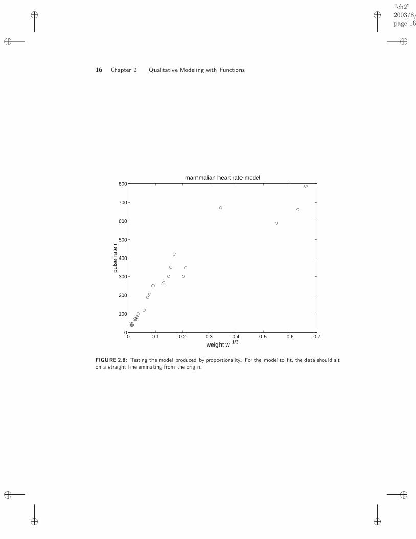
r = kw−1/3

To validate this model we plot w−1/3 versus r for the data Table 2.8. We seethat for the larger animals with slower heart rates that this data appears linearand suggests this rather crude model actually is supported by the data. For muchsmaller animals there appear to be factors that this model is not capturing and thedata falls off the line.

2.4 DIMENSIONAL ANALYSIS

In this chapter we have explored modeling with functions and proportion. In someinstances, such as the mammalian heart rate, it is possible to cobble enough infor-mation together to actually extract a model; in particular, to identify the functionalform for the relationship between the dependent and independent variables. Nowwe turn to a surprisingly powerful and simple tool known as dimensional analysis1.

Dimensional analysis operates on the premise that equations contain termsthat have units of measurement and that the validity of these equations, or laws,are not dependent on the system of measurement. Rather these equations relatevariables that have inherent physical dimensions that are derived from the funda-mental dimensions of mass, length and time. We label these dimensions genericallyas M, L and T , respectively.

As we shall see, dimensional analysis provides an effective tool for mathemat-ical modeling in many situations. In particular, some benefits include

1This dimension should not be confused with the usual notion of geometric dimension.

“ch2”2003/8/page 16


0 0.1 0.2 0.3 0.4 0.5 0.6 0.70

100

200

300

400

500

600

700

800

puls

e ra

te r

weight w−1/3

mammalian heart rate model

FIGURE 2.8: Testing the model produced by proportionality. For the model to fit, the data should siton a straight line eminating from the origin.

“ch2”2003/8/page 17


• determination of the form of a joint proportion

• reduce number of variables in a model

• enforcement of dimensional consistency

• ability to study scaled versions of models

2.4.1 Dimensional homogeneity

An equation is said to be dimensionally homogeneous if all the terms in the equationhave the same physical dimension.

EXAMPLE 2.12

All the laws of physics are dimensionally homogeneous. Consider Newton’s law

F = ma

The units on the right side are

M · L

T 2

so we conclude that the physical dimension of a force must be MLT−2. �

EXAMPLE 2.13

The equation of motion of a linear spring with no damping is

md2x

dt2+ kx = 0

What are the units of the spring constant? Dimensionally we can recast this equa-tion as

MLT−2 + MaLbT cL = 0

Matching exponents for each dimension permits the calculation of a, b and c.

M : a = 1L : 1 = b + 1T : − 2 = c

Thus we conclude that the spring constant has the dimensions MT−2. �

EXAMPLE 2.14

Let v be velocity, t be time and x be distance. The model equation

v2 = t2 +x

t

is dimensionally inconsistent.

“ch2”2003/8/page 18


EXAMPLE 2.15

An angle may be defined by the formula

θ =s

r

where the arclength s subtends the angle θ and r is the radius of the circle. Clearlythis angle is dimensionless.

2.4.2 Discovering Joint Proportions

If in the formulation of a problem we are able to identify a dependent and oneor more independent variables, it is often possible to identify the form of a jointproportion. The form of the proportion is actually constrained by the fact that theequations must be dimensionally consistent.

EXAMPLE 2.16 Drag Force on an Airplane

In this problem we consider the drag force FD on an airplane. As our model wepropose that this drag force (dependent variable) is proportional to the independentvariables

• cross-sectional area A of airplane

• velocity v of airplane

• density ρ of the air

As a joint proportion we have

FD = kAavbρc

where a, b and c are unknown exponents. As a consequence of dimensional consis-tency we have

MLT−2 = (M0L0T 0)(L2)a(L

T)b(

M

L3)c

= M cL2a−3c+bT−b

From the M exponent we conclude c = 1. From the T exponent b = 2 andfrom the L exponent it follows that 1 = 2a− 3c + b, whence a = 1. Thus the onlypossibility for the form of this joint proportion is

FD = kAv2ρ

Note that if the density of were a constant it would be appropriate to simplify thisdependency as

F = kAv2

but now the constant k actually has dimensions. �

“ch2”2003/8/page 19


2.4.3 Procedure for Nondimensionalization

Consider the nonlinear model for a pendulum

d2θ

dt2= −g

lsin θ

Based on the terms in this model we may express the solution very generally as arelationship between these included terms, i.e.,

φ(θ, g, l, t) = 0

Note that the angle in this model is dimensionless but the other variables allhave dimensions. We can convert this equation into a new equation where noneof the terms have dimensions. This will be referred to, for obvious reasons, as adimensional form of the model.

To accomplish this, let

τ =t√l/g

.

The substitution of variables may be accomplished by noting that

d2θ

dt2=

d2θlg dτ2

Thus, after cancelation, the dimensionless form for the nonlinear pendulum modelis

d2θ

dτ2= − sin θ

Now the solution has the general form

f(θ, τ) = 0,

or equivalently,

f(θ,

√l

gt) = 0

This is a special case of a more general theory.The Buckingham π-theorem. Any dimensionally homogeneous equation with

physical variables x1, . . . , xm expressed

φ(x1, . . . , xm)

may be rewritten in terms of its associated dimensionless variables π1, . . . , πn as

f(π1, . . . , πn) = 0

whereπk = xak1

1 . . . xakmm

“ch2”2003/8/page 20


2.4.4 Modeling with Dimensional Analysis

Now we consider two examples of the application of the ideas described aboveconcerning dimensional analysis. In each of these examples there is more than onedimensionless parameter and it is appropriate to apply the Buckingham π-theorem.

The Pendulum. In this example the goal is to understand how the periodof a pendulum depends on the other parameters that describe the nature of thependulum. The first task is to identify this set of parameters that act as theindependent variables on which the period P depends.

Obvious candidates include From this list we are motivated to write

variable symbol dimensionsmass m Mlength l Lgravity g LT−2

angle θ0 M0L0T 0

period P T

TABLE 2.2: Parameters influencing the motion of a simple pendulum.

P = φ(m, l, g, θ0)

As we shall see, attempting to establish the form of φ directly is unnecessarilycomplicated. Instead, we pursue the idea of dimensional analysis.

To begin this modeling procedure, we compute the values of a, b, c, d and ethat make the quantity

π = malbgcθd0P e

a dimensionless parameter. Again, this is done by equating exponents on the fun-damental dimensions

M0L0T 0 = MaLb(LT−2)c(M0L0T 0)dT e

From M0: 0 = a.From L0: 0 = b + c.From T 0: 0 = −2c + e.From this we may conclude that

π = m0l−cgcθd0P 2c

or, after collecting terms,

π = θd0

(gP 2

l

)c

where π is dimensionless for any values of d and c. Thus we have found a completeset of dimensionless parameters

π1 = θ0

“ch2”2003/8/page 21


and

π2 =√

g

lP

Since the period P of the pendulum is based on dimensionally consistentphysical laws we may apply the Buckingham π-theorem. In general,

f(π1, π2) = 0

which we rewrite asπ2 = h(π1)

which now becomes

P =

√l

gh(θ0)

We may draw two immediate conclusions from this model.

• The period depends on the square root of the length of the pendulum.

• The period is independent of the mass

Of course we have not really shown these conclusions to be ”true”. But now we havesomething to look for that can be tested. We could test these assertions and if theycontradict our model then we would conclude that we are missing an importantfactor that governs the period of the pendulum. Indeed, as we have neglected dragforces due to friction it seems our model will have limited validity.

The functional form of h may now be reasonable calculated as there is onlyone independent variable θ0. If we select several different initial displacements θ0(i)and measure the period for each one we have a set of domain–range values

h(θ0(i)) = Pi

√g

l

to which a data fitting procedure may now be applied.

The damped pendulum. We assumed that there was no damping of thispendulum above due to air resistance. We can include a drag force FD by aug-menting the list of relevant parameters to

m, l, g, θ0, P, FD

Now our dimensionless parameter takes the form

π = malbgcθd0P eF f

D

Converting to dimensions

M0L0T 0 = MaLb(LT−2)c(M0L0T 0)dT e(MLT−2)f

As0 = a + f

“ch2”2003/8/page 22


it is no longer possible to immediately conclude that a = 0. In fact, it is not. (Seeproblems).

Fluid Flow. Consider the parameters governing the motion of an oil pasta spherical ball bearing. Let’s assume they include:

variable symbol dimensionsvelocity v LT−1

density ρ ML−3

gravity g LT−2

radius l Lviscosity µ ML−1T−1

TABLE 2.3: Parameters influencing the motion of a fluid around a submerged body.

The dimensionless combination has the form

π = vaρblcgdµe

Using the explicit form of the physical dimensions for each term we have

M0L0T 0 = (LT−1)a(ML−3)b(L)c(LT−2)d(ML−1T−1)e

Again, matching exponentsM : 0 = b + e

L : 0 = a− 3b + c + d− e

T : 0 = −a− 2d− e

Sinc there are three equations and five unknowns the system is said to be unde-termined. Given these numbers, we anticipate that there we can solve for threevariable in terms of the other two. Of course, we can solve in terms of any of thetwo variables. For example,

a = −2d− e

b = −e

c = d− e

Plugging these constraints into our expression for π gives

π =(v2

lg

)−d(ρlv

µ

)−e

Thus, our two dimensionless parameters are the Froude number

π1 =v2

lg

and the Reynolds number

π2 =vρl

µ

For further discussion see Giordano, Wells and Wilde, UMAP module 526.

“ch2”2003/8/2page 23


PROBLEMS

2.1. By drawing a new graph, show the effect of the size of the island on the

• extinction curve

• migration curve

Now predict how island size impacts the number of species on the island. Doesthis seem reasonable?

2.2. Give an example of a commodity that does not obey the

• law of supply

• law of demand

and justify your claim.2.3. Translate into words the qualitative interpretation of the slope of the supply and

demand curves. In particular, what is the meaning of a

• flat supply curve?

• steep supply curve?

• steep demand curve?

2.4. Consider the table of market adjustments below. Assuming the first point ison the demand curve, compute the equations of both the demand and supplycurve. Using these equations, find the missing values A, B, C, D. What is theequilibrium point? Do you think the market will adjust to it?

quantity price3 0.7

0.14 0.70.14 0.986

0.1972 0.986A =? B =?C =? D =?

2.5. Using the cobweb plot show an example of a market adjustment that oscillateswildly out of control. Can you describe a qualitative feature of the supply anddemand curves that will ensure convergence to an equilibrium?

2.6. Consider the effect of a price increase on airplane fuel (kerosene) on the airlineindustry. What effect does this have on the supply curve? Will the airlineindustry be able to pass this cost onto the flying public? How does your answerdiffer if the demand curve is flat versus steep?

2.7. Prove properties 2.1 and 2.2.2.8. Is the temperature measured in degrees Fahrenheit proportional to the temper-

ature measured in degrees centigrade?2.9. Consider the Example 2.6 again. Demonstrate the proportionalities stated. For

the case of the breaking distance equate the work done by the breaks to thedissipated kinetic energy of the car.

2.10. Items at the grocery store typically come in various sizes and the cost per unit isgenerally smaller for larger items. Model the cost per unit weight by consideringthe superposition of proportions due to the costs of

• production

• packaging

“ch2”2003/8/2page 24


• shipping

the product. What predictions can you make from this model. This problemwas adapted from Bender [1].

2.11. Go to your nearest supermarket and collect data on the cost of items as a functionof size. Do these data behave in a fashion predicted by your model in the previousproblem?

2.12. In this problem take the diagonal of a rectangle as it’s length scale l. Show bydirect calculation that this can be used to measure the area, i.e.,

A = αl2

Determine the constant of proportionality α in terms of the shape factor of therectangle.

2.13. Consider a radiator designed as a spherical shell. If the characteristic lengthof the shell doubles (assume the larger radiator is geometrically similar to thesmaller radiator) what is the effect on the amount of heat loss? What if thedesign of the radiator is a parallelpiped instead?

2.14. How does the argument in Example 2.10 change if the falling object is not spher-ical but some other irregular shape?

2.15. Extend the definition of geometric similarity for

• parallelpipeds

• irregularly shaped objects

Can you propose a computer algorithm for testing whether two objects are ge-omtrically similar?

2.16. Consider the force on a pendulum due to air friction modeled by

FD = κv2

Determine the units of κ.2.17. Newton’s law of gravitation states that

F = Gm1m2

r2

where F is the force between two objects of masses m1, m2 and r is the distancebetween them.(a) What is the physical dimension of G?(b) Compute two dimensionless products π1 and π2 and show explicitly that

they satisfy the Buckingham π-theorem.2.18. This problem concerns the pendulum example described in subsection 2.4.4. Re-

peat the analysis to determine the dimensionless parameter(s) but now omit thegravity term g. Discuss.

2.19. This problem concerns the pendulum example described in subsection 2.4.4. Re-peat the analysis for determining all the dimensionless parameters but now in-clude a parameter κ associated with the drag force of the form FD = κv. Hint:first compute the dimensions of κ.

2.20. Convert the equation governing the distance traveled by a projectile

d2x

dt2= −gR2

(x + R)2

“ch2”2003/8/page 25


with the initial conditions

x(0) = 0dx

dt(0) = V

to non-dimensional form using the transformation

y =x

Rτ =

V t

R

Verify the resulting equation is dimensionless. See [4] for further details.2.21. Reconsider the example in subsection 2.4.4. Instead of solving for a, b, c in terms

of d, e solve for c, d, e in terms of a and b. Show that now

π′1 = v√

lg

and

π′2 = ρl3/2g1/2

µ

Show also that both π′1 and π

′2 can be written in terms of π1 and π2.

2.22. Consider an object with surface area A traveling with a velocity v through amedium with kinematic viscosity µ and density ρ.(a) Assuming the effect of µ is small compute the drag force due to the density

Fρ.(b) Assuming the effect of ρ is small compute the drag force due to the kinematic

viscosity Fµ.c) Compute the dimensionless ratio of these drag forces and discuss what pre-

dictions you can make.2.23. How does the required power P of a helicopter engine depend on the length of the

rotors l? The rotors are pushing air so presumable the density ρ as well as theweight of the helicopter w = mg are variables that affect the power requirement.Draw a sketch of your result plotting P versus l. See [3] for more discussion ofthis problem.

“ch2”2003/8/page 26

Bibliography

1. Edward A. Bender. An Introduction to Mathematical Modeling. John Wiley & Sons,New York, 1978.

2. F.R. Giordano, M.D. Weir, and W.P. Fox. A First Course in Mathematical Modeling.Brooks/Cole, Pacific Grove, 1997.

3. T.W. Korner. The Pleasures of Counting. Cambridge University Press, Cambridge,U.K., 1996.

4. C.C. Lin and L.A. Segel. Mathematics Applied to Deterministic Problems in the NaturalSciences. Macmillan, New York, 1974.

26

ch2 - whitman people

Documents