ch15 urban streets - againc.net · highway capacity manual 2000 15-1 chapter 15 - urban streets...

Highway Capacity Manual 2000

15-i Chapter 15 - Urban Streets

CHAPTER 15

URBAN STREETS

CONTENTS

I. INTRODUCTION..................................................................................................... 15-1Scope of the Methodology................................................................................ 15-1Limitations of the Methodology ........................................................................ 15-1

II. METHODOLOGY .................................................................................................... 15-1LOS .................................................................................................................. 15-2Determining Urban Street Class ...................................................................... 15-3Determining Running Time .............................................................................. 15-3Determining Delay ............................................................................................ 15-3

Uniform Delay ........................................................................................... 15-5Incremental Delay ..................................................................................... 15-5Initial Queue Delay .................................................................................... 15-5Arrival Type and Platoon Ratio ................................................................. 15-5Progression Adjustment Factor................................................................. 15-6Incremental Delay Adjustment for Actuated Controls ............................... 15-7Upstream Filtering or Metering Adjustment Factor, I ................................ 15-8

Determining Travel Speed................................................................................ 15-8Determining LOS.............................................................................................. 15-9Sensitivity of Results to Input Variables ........................................................... 15-9

III. APPLICATIONS .................................................................................................... 15-12Segmenting the Urban Street......................................................................... 15-13Computational Steps ...................................................................................... 15-13Planning Applications ..................................................................................... 15-14Analysis Tools ................................................................................................ 15-15

IV. EXAMPLE PROBLEMS ........................................................................................ 15-15Example Problem 1 ........................................................................................ 15-16Example Problem 2 ........................................................................................ 15-18Example Problem 3 ........................................................................................ 15-20Example Problem 4 ........................................................................................ 15-22Example Problem 5 ........................................................................................ 15-24

APPENDIX A. PLANNING APPLICATION COMPUTATIONS ................................... 15-25APPENDIX B. TRAVEL TIME STUDIES FOR DETERMINING LOS ......................... 15-27APPENDIX C. WORKSHEETS................................................................................... 15-28

Urban Street WorksheetTravel-Time Field Worksheet

EXHIBITS

Exhibit 15-1. Urban Street Methodology .................................................................... 15-2Exhibit 15-2. Urban Street LOS by Class ................................................................... 15-3Exhibit 15-3. Segment Running Time per Kilometer .................................................. 15-4Exhibit 15-4. Relationship Between Arrival Type and Platoon Ratio (Rp) .................. 15-6Exhibit 15-5. Progression Adjustment Factors for Uniform Delay Calculation ........... 15-7Exhibit 15-6. k-Value for Controller Type.................................................................... 15-8Exhibit 15-7. Recommended I-Values for Lane Groups with Upstream Signals ........ 15-8Exhibit 15-8. Speed-Flow Curves for Class I Urban Streets .................................... 15-10Exhibit 15-9. Speed-Flow Curves for Class II Urban Streets ................................... 15-10


Chapter 15 - Urban Streets 15-ii

Exhibit 15-10. Speed-Flow Curves for Class III Urban Streets .................................. 15-11Exhibit 15-11. Speed-Flow Curves for Class IV Urban Streets .................................. 15-11Exhibit 15-12. Change in Mean Speed for Arrival Types ........................................... 15-12Exhibit 15-13. Types of Urban Street Segments ........................................................ 15-13Exhibit 15-14. Urban Street Worksheet...................................................................... 15-14Exhibit A15-1. Urban Street LOS Calculations ........................................................... 15-26Exhibit B15-1. Travel-Time Field Worksheet .............................................................. 15-28


15-1 Chapter 15 - Urban StreetsIntroduction

I. INTRODUCTION

SCOPE OF THE METHODOLOGYBackground and underlyingconcepts for this chapter arein Chapter 10

This chapter provides a methodology for analyzing urban streets. This methodologyalso may be used to analyze suburban streets that have a traffic signal spacing of 3.0 kmor less. Both one-way and two-way streets can be analyzed with this methodology;however, each travel direction of the two-way street requires a separate analysis.

The methodology described in this chapter can be used to assess mobility on anurban street. The degree of mobility provided is assessed in terms of travel speed for thethrough-traffic stream. A street’s access is not assessed with this methodology.However, the level of access provided by a street also should be considered whenevaluating its performance, especially if the street is intended to provide access. Factorsthat favor mobility often reflect minimal levels of access and vice versa.

The methodology described in this chapter focuses on mobility; urban streets withmobility tend to be at least 3 km long (or in downtown areas, 1.5 km). A shorter streetalso may be analyzed; however, it is likelier that its primary function is access. Accesscan be evaluated to some degree through an analysis of the individual intersections alongthe street.

LIMITATIONS OF THE METHODOLOGY

The urban streets methodology does not directly account for the following conditionsthat can occur between intersections:

• Presence or lack of on-street parking;• Driveway density or access control;• Lane additions leading up to, or lane drops leading away from, intersections;• The impact of grades between intersections;• Any capacity constraints between intersections (such as a narrow bridge);• Midblock medians and two-way left-turn lanes;• Turning movements that exceed 20 percent of the total volume on the street;

For queue estimation method,see Chapter 16, Appendix G

• Queues at one intersection backing up to and interfering with the operation of anupstream intersection; and

• Cross-street congestion blocking through traffic.Because any one of these conditions might have a significant impact on the speed of

through traffic, the analyst should modify the methodology to incorporate the effects asbest as possible.

II. METHODOLOGY

This methodology provides the framework for the evaluation of urban streets. Iffield data on travel times are available, this framework can be used to determine thestreet’s level of service (LOS). Also, the direct measurement of the travel speed along anurban street can provide an accurate estimate of LOS without using the computationspresented in this chapter.

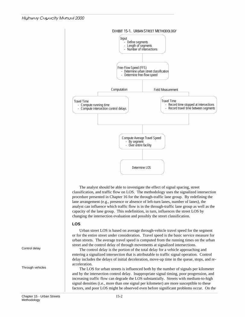
Urban street traffic models can be used as alternative sources for field data, providedthat the input parameters—such as running times and saturation flow rates—aredetermined according to the procedures in this manual, and that the calculated orestimated delay and the delay outputs are based on the definitions and equations in thismanual or have been validated by field data. Exhibit 15-1 illustrates the basic method fordetermining LOS on an urban street.

Chapter 15 - Urban Streets 15-2Methodology

EXHIBIT 15-1. URBAN STREET METHODOLOGY

Input- Define segments- Length of segments- Number of intersections

Free-Flow Speed (FFS)- Determine urban street classification- Determine free-flow speed

Travel Time- Compute running time- Compute intersection control delays

Travel Time- Record time stopped at intersections- Record travel time between segments

Compute Average Travel Speed- By segment- Over entire facility

Determine LOS

Computation Field Measurement

The analyst should be able to investigate the effect of signal spacing, streetclassification, and traffic flow on LOS. The methodology uses the signalized intersectionprocedure presented in Chapter 16 for the through-traffic lane group. By redefining thelane arrangement (e.g., presence or absence of left-turn lanes, number of lanes), theanalyst can influence which traffic flow is in the through-traffic lane group as well as thecapacity of the lane group. This redefinition, in turn, influences the street LOS bychanging the intersection evaluation and possibly the street classification.

LOS

Urban street LOS is based on average through-vehicle travel speed for the segmentor for the entire street under consideration. Travel speed is the basic service measure forurban streets. The average travel speed is computed from the running times on the urbanstreet and the control delay of through movements at signalized intersections.

Control delay The control delay is the portion of the total delay for a vehicle approaching andentering a signalized intersection that is attributable to traffic signal operation. Controldelay includes the delays of initial deceleration, move-up time in the queue, stops, and re-acceleration.

Through vehicles The LOS for urban streets is influenced both by the number of signals per kilometerand by the intersection control delay. Inappropriate signal timing, poor progression, andincreasing traffic flow can degrade the LOS substantially. Streets with medium-to-highsignal densities (i.e., more than one signal per kilometer) are more susceptible to thesefactors, and poor LOS might be observed even before significant problems occur. On the



15-3 Chapter 15 - Urban StreetsMethodology

other hand, longer urban street segments comprising heavily loaded intersections canprovide reasonably good LOS, although an individual signalized intersection might beoperating at a lower level. The term through vehicle refers to all vehicles passing directlythrough a street segment and not turning.

Exhibit 15-2 lists urban street LOS criteria based on average travel speed and urbanstreet class. It should be noted that if demand volume exceeds capacity at any point onthe facility, the average travel speed might not be a good measure of the LOS. The streetclassifications identified in Exhibit 15-2 are defined in the next section.

EXHIBIT 15-2. URBAN STREET LOS BY CLASSTravel speed defines LOS onurban streets

Urban Street Class I II III IV

Range of free-flowspeeds (FFS)

90 to 70 km/h 70 to 55 km/h 55 to 50 km/h 55 to 40 km/h

Typical FFS 80 km/h 65 km/h 55 km/h 45 km/h

LOS Average Travel Speed (km/h)

A > 72 > 59 > 50 > 41B > 56–72 > 46–59 > 39–50 > 32–41C > 40–56 > 33–46 > 28–39 > 23–32D > 32–40 > 26–33 > 22–28 > 18–23E > 26–32 > 21–26 > 17–22 > 14–18F ≤ 26 ≤ 21 ≤ 17 ≤ 14

DETERMINING URBAN STREET CLASS

The first step in the analysis is to determine the urban street’s class. This can bebased on direct field measurement of the FFS or on an assessment of the subject street’sfunctional and design categories. A procedure for measuring the FFS is described inAppendix B.

If the FFS measurements are not available, the street’s functional and designcategories must be used to identify its class. The functional category is identified first,followed by the design category. This identification uses the definitions provided inChapter 10 and Exhibit 10-4. After determining the functional and design categories, theurban street class can be established using Exhibit 10-3.

DETERMINING RUNNING TIMERunning time is estimatedusing FFS, urban streetclassification, and arterialsegment length

There are two principal components of the total time that a vehicle spends on asegment of an urban street: running time and control delay at signalized intersections. Tocompute the running time for a segment, the analyst must know the street’s classification,its segment length, and its FFS. The segment running time then can be found by usingExhibit 15-3.

Within each urban street class there are several influences on actual running time.Exhibit 15-3 shows the effect of street length. In addition, the presence of parking, sidefriction, local development, and street use can affect running time. In this chapter, thesealso are assumed to influence the FFS. Direct observation of the FFS, therefore, includesthe effect of these factors and, by implication, their effect on the running speed.

If it is not possible to observe the FFS on the actual or a comparable facility, defaultvalues are given in a note to Exhibit 15-3.

DETERMINING DELAY

Computing the urban street or section speed requires the intersection control delays.Because the function of an urban street is to serve through traffic, the lane group forthrough traffic is used to characterize the urban street.



EXHIBIT 15-3. SEGMENT RUNNING TIME PER KILOMETER

Urban Street Class I II III IV

FFS (km/h) 90a 80a 70a 70a 65a 55a 55a 50a 55a 50a 40a

Average SegmentLength (m)

Running Time per Kilometer (s/km)

100 b b b b b b - - - 129 159200 b b b b b b 88 91 97 99 125400 59 63 67 66 68 75 75 78 77 81 96600 52 55 61 60 61 67 d d d d d

800 45 49 57 56 58 65 d d d d d

1000 44 48 56 55 57 65 d d d d d

1200 43 47 54 54 57 65 d d d d d

1400 41 46 53 53 56 65 d d d d d

1600 40c 45c 51c 51c 55c 65c d d d d d

Notes:a. It is best to have an estimate of FFS. If there is none, use the table above, assuming the following default values:

For Class FFS (km/h)I 80II 65III 55IV 45

b. If a Class I or II urban street has a segment length less than 400 m, (a) reevaluate the class and (b) if it remains a distinctsegment, use the values for 400 m.c. For long segment lengths on Class I or II urban streets (1600 m or longer), FFS may be used to compute running time perkilometer. These times are shown in the entries for a 1600-m segment.d. Likewise, Class III or IV urban streets with segment lengths greater than 400 m should first be reevaluated (i.e., theclassification should be confirmed). If necessary, the values above 400 m can be extrapolated.Although this table does not show it, segment running time depends on traffic flow rates; however, the dependence ofintersection delay on traffic flow rate is greater and dominates in the computation of travel speed.

The control delay for the through movement is the appropriate delay to use in anurban street evaluation. In general, the analyst should have this information because theintersections should have been evaluated individually as part of the overall analysis.Equation 15-1 is used to compute control delay. Equations 15-2 and 15-3 are used tocompute uniform delay and incremental delay, respectively.

d = d1(PF) + d2 + d3 (15-1)

d1 =0.5C 1 − g

C

2

1 − min(1,X )gC

(15-2)

d2 = 900T (X −1) + (X −1)2 + 8k l XcT

(15-3)

whered = control delay (s/veh);

d1 = uniform delay (s/veh);d2 = incremental delay (s/veh);d3 = initial queue delay, see Chapter 16 (s/veh);

PF = progression adjustment factor (Exhibit 15-5);X = volume to capacity (v/c) ratio for the lane group (also termed degree of

saturation);C = cycle length (s);c = capacity of lane group (veh/h);g = effective green time for lane group (s);T = duration of analysis period (h);



k = incremental delay adjustment for the actuated control; andI = incremental delay adjustment for the filtering or metering by upstream

signals.

Uniform DelayThe v/c ratio (X) for a lanegroup cannot be greater than1.0 to compute uniform delay

Equation 15-2 gives an estimate of control delay assuming perfectly uniform arrivalsand a stable flow. It is based on the first term of Webster's delay formulation and isaccepted as an accurate depiction of delay for the ideal case of uniform arrivals. Valuesof X greater than 1.0 are not used in the computation of d1.

Incremental Delay

Equation 15-3 estimates the incremental delay due to nonuniform arrivals andindividual cycle failures (i.e., random delay) as well as delay caused by sustained periodsof oversaturation (i.e., oversaturation delay). The equation interrelates the degree ofsaturation (X) of the lane group, the duration of the analysis (T), the capacity of the lanegroup (c), and the signal control (k). The equation assumes that all demand flow has beenserviced in the previous analysis period—that is, there is no initial queue. If there is,Appendix F of Chapter 16 offers procedures to account for the effect of an initial queue.The incremental delay term is valid for all degrees of saturation.

Initial Queue DelaySee also Appendix F ofChapter 16

When a queue from the previous period is present at the start of the analysis, newlyarriving vehicles experience initial queue delay. This delay results from the additionaltime required to clear the initial queue. Its magnitude depends on the size of the initialqueue, the length of the analysis period, and the v/c ratio for that period. A procedure fordetermining the initial queue delay also is described in Appendix F of Chapter 16.

Arrival Type and Platoon Ratio

A critical characteristic that must be quantified for the analysis of an urban street orsignalized intersection is the quality of the progression. The parameter that describes thischaracteristic is the arrival type, AT, for each lane group. This parameter approximatesthe quality of progression by defining six types of dominant arrival flow.

Six arrival typesArrival Type 1 is characterized by a dense platoon of more than 80 percent of thelane group volume arriving at the start of the red phase. This arrival type representsnetwork links that experience a poor rate of progression due to various conditions,including lack of coordination.

Arrival Type 2 is characterized by a moderately dense platoon that arrives in themiddle of the red phase or by a dispersed platoon of 40 to 80 percent of the lane groupvolume arriving throughout the red phase. This arrival type represents an unfavorableprogression along an urban street.

Arrival Type 3 consists of random arrivals in which the main platoon contains lessthan 40 percent of the lane group volume. This arrival type represents operations atnoninterconnected, signalized intersections with highly dispersed platoons. It also maybe used to represent a coordinated operation with minimal benefits of progression.

Arrival Type 4 consists of a moderately dense platoon that arrives in the middle ofthe green phase or of a dispersed platoon of 40 to 80 percent of the lane group volumearriving throughout the green phase. This arrival type represents a favorable progressionalong an urban street.

Arrival Type 5 is characterized by a dense to moderately dense platoon of more than80 percent of the lane group volume arriving at the start of the green phase. This arrivaltype represents a highly favorable progression, which may occur on routes with a low-to-moderate number of side street entries and which receive high priority in signal timing.



Arrival Type 6 is reserved for exceptional progression quality on routes with near-ideal characteristics. It represents dense platoons progressing over several closely spacedintersections with minimal or negligible side street entries.

Arrival type is best observed in the field but can be approximated by examiningtime-space diagrams for the street. The arrival type should be determined as accuratelyas possible because it has a significant impact on delay estimates and LOS determination.Although there are no definitive parameters to quantify arrival type, the ratio defined byEquation 15-4 is useful.

Rp = PCg

(15-4)

whereRP = platoon ratio,P = proportion of all vehicles arriving during green,C = cycle length (s), andg = effective green time for movement (s).

The value for P may be estimated or observed in the field, whereas C and g arecomputed from the signal timing. The value of P may not exceed 1.0. The approximateranges of Rp relate to arrival type as shown in Exhibit 15-4, which also suggests defaultvalues for use in subsequent computations.

EXHIBIT 15-4. RELATIONSHIP BETWEEN ARRIVAL TYPE AND PLATOON RATIO (Rp)

Arrival Type Range of Platoon Ratio (RP) Default Value (RP) Progression Quality

1 ≤ 0.50 0.333 Very poor2 > 0.50–0.85 0.667 Unfavorable3 > 0.85–1.15 1.000 Random arrivals4 > 1.15–1.50 1.333 Favorable5 > 1.50–2.00 1.667 Highly favorable6 > 2.00 2.000 Exceptional

Progression Adjustment Factor

Good signal progression results in the arrival of a high proportion of vehicles on thegreen; poor signal progression results in the arrival of a low proportion of vehicles on thegreen. The progression adjustment factor, PF, applies to all coordinated lane groups,whether the control is pretimed or nonactuated in a semiactuated system. Progressionprimarily affects uniform delay; for this reason, the adjustment is applied only to d1. Thevalue of PF may be determined by Equation 15-5.

PF =1 − P( )fPA

1 − gC

(15-5)

wherePF = progression adjustment factor,

P = proportion of all vehicles arriving during green,g/C = effective green-time ratio, andfPA = supplemental adjustment factor for platoon arrival during the green.

The value of P may be measured in the field or estimated from the time-spacediagram. The value of PF also may be computed from measured values of P using thedefault values for fPA. Alternatively, Exhibit 15-5 may be used to determine PF as afunction of the arrival type based on the default values for P and fPA associated with eacharrival type. If PF is estimated by Equation 15-5, its value may not exceed 1.0 for Arrival



Type 4 with extremely low values of g/C; as a practical matter, PF should be assigned amaximum value of 1.0 for Arrival Type 4.

EXHIBIT 15-5. PROGRESSION ADJUSTMENT FACTORS FOR UNIFORM DELAY CALCULATION

Arrival Type (AT)

Green Ratio(g/C)

AT 1 AT 2 AT 3 AT 4 AT 5 AT 6

0.20 1.167 1.007 1.000 1.000 0.833 0.7500.30 1.286 1.063 1.000 0.986 0.714 0.5710.40 1.445 1.136 1.000 0.895 0.555 0.3330.50 1.667 1.240 1.000 0.767 0.333 0.0000.60 2.001 1.395 1.000 0.576 0.000 0.0000.70 2.556 1.653 1.000 0.256 0.000 0.000

fPA 1.00 0.93 1.00 1.15 1.00 1.00

Default, Rp 0.333 0.667 1.000 1.333 1.667 2.000

Notes:PF = (1 – P)fPA/(1 – g/C).Tabulation is based on default values of fp and Rp.P = Rp * g/C (may not exceed 1.0).PF may not exceed 1.0 for AT 3 through AT 6.

Guidelines on arrival type forfuture conditions

The progression adjustment factor, PF, requires knowledge of offsets, travel speeds,and intersection signalization. When delay is estimated for future coordination,particularly when analyzing alternatives, Arrival Type 4 should be assumed as a basecondition for coordinated lane groups (except for left turns), and Arrival Type 3 shouldbe assumed for all uncoordinated lane groups.

For movements made from exclusive left-turn lanes on exclusive phases, theprogression adjustment factor usually should be 1.0 (i.e., Arrival Type 3). However, ifthe signal coordination provides for a progression of left-turn movements, the progressionadjustment factor should be computed from the estimated arrival type, as for throughmovements. When the coordinated left turn is part of protected-permitted phasing, onlythe effective green for the protected phase should be used to determine the progressionadjustment factor, since the protected phase normally is associated with platoonedcoordination. A flow-weighted average of P should be used in determining PF when atime-space diagram is used and lane group movements have different levels ofcoordination.

Incremental Delay Adjustment for Actuated ControlsFor pretimed signals, k = 0.50In Equation 15-3 the term k incorporates the effect of the controller on delay. For

pretimed signals, a k-value of 0.50 is used. This is based on queuing with randomarrivals and on uniform service equivalent to the lane group capacity. Actuatedcontrollers, however, can tailor the green time to the current demand, reducing the overallincremental delay. The delay reduction depends in part on the controller’s unit extensionand the degree of saturation. Research has indicated that lower unit extensions (i.e.,snappy intersection operation) result in lower values of k and d2. However, when the

degree of saturation approaches 1.0, an actuated controller will act like a pretimedcontroller, producing k-values of 0.50 at degrees of saturation greater than or equal to1.0. Exhibit 15-6 illustrates the k-values recommended for actuated controllers withdifferent unit extensions and degrees of saturation.

For unit extension values not listed in Exhibit 15-6, the k-values may be interpolated.If the formula in Exhibit 15-6 is used, the kmin value (i.e., the k-value for X = 0.50) first

should be interpolated for the unit extension and then the formula should be used.Exhibit 15-6 may be extrapolated for unit extension values beyond 5.0 s, but theextrapolated k-value never should exceed 0.50.


EXHIBIT 15-6. k-VALUE FOR CONTROLLER TYPE

Degree of Saturation (X)

Unit Extension (s) ≤ 0.50 0.60 0.70 0.80 0.90 ≥ 1.0

≤ 2.0 0.04 0.13 0.22 0.32 0.41 0.502.5 0.08 0.16 0.25 0.33 0.42 0.503.0 0.11 0.19 0.27 0.34 0.42 0.503.5 0.13 0.20 0.28 0.35 0.43 0.504.0 0.15 0.22 0.29 0.36 0.43 0.504.5 0.19 0.25 0.31 0.38 0.44 0.505.0a 0.23 0.28 0.34 0.39 0.45 0.50

Pretimed orNonactuated Movement

0.50 0.50 0.50 0.50 0.50 0.50

Notes:For a unit extension and its kmin value at X = 0.5: k = (1 – 2kmin)(X – 0.5) + kmin, where k ≥ kmin, and k ≤ 0.5.a. For a unit extension more than > 5.0, extrapolate to find k, keeping k ≤ 0.5.

Upstream Filtering or Metering Adjustment Factor, I

The incremental delay adjustment term I in Equation 15-4 accounts for the effects offiltered arrivals from upstream signals. An I-value of 1.0 is used for an isolatedintersection (i.e., one that is 1.6 km or more from the nearest upstream signalizedintersection). This value is based on a random number of vehicles arriving per cycle sothat the variance in arrivals equals the mean.

An I-value of less than 1.0 is used for nonisolated intersections. This reflects theway that upstream signals decrease the variance in the number of arrivals per cycle at thesubject (i.e., downstream) intersection. As a result, the amount of delay due to randomarrivals is reduced.

Exhibit 15-7 lists I-values for nonisolated intersections. The values of I in thisexhibit are based on Xu, the weighted v/c ratio of all upstream movements contributing to

the volume in the subject intersection lane group. This ratio is computed as a weightedaverage with the v/c ratio of each contributing upstream movement weighted by itsvolume. For the analysis of urban street performance, it is sufficient to approximate Xuas the v/c ratio of the upstream through movement.

EXHIBIT 15-7. RECOMMENDED I-VALUES FOR LANE GROUPS WITH UPSTREAM SIGNALS

Degree of Saturation at Upstream Intersection, Xu

0.40 0.50 0.60 0.70 0.80 0.90 ≥ 1.0

I 0.922 0.858 0.769 0.650 0.500 0.314 0.090

Note: I = 1.0 – 0.91 Xu2.68 and Xu ≤ 1.0.

DETERMINING TRAVEL SPEED

Equation 15-6a is used to compute the average travel speed for a segment.

SA =

3600LTR + d + dm

(15-6a)

whereSA = average travel speed of through vehicles in the segment (km/h);

L = segment length (km);TR = running time on the segment (= tRL) (s);tR = running time per kilometer along the segment, from Exhibit 15-3

(s/km);


15-8a Chapter 15 - Urban StreetsMethodology

d = control delay for through movements at the signalized intersection atthe end of the segment (s); and

dm = delay for through movements at locations other than the signalizedintersection (e.g., midblock delay) (s).

Equation 15-6b is used to compute the average travel speed for the urban street.

SA =

3600 (L)∑(∑ TR + d + dm )

(15-6b)

When using this equation, the length of each segment on the urban street is added toobtain a total street length, (L)∑ . Similarly, the individual running times and delays of

each segment are added to obtain a total travel time, (TR + d + dm)∑ .



DETERMINING LOS

There is a distinct set of urban street LOS criteria for each urban street class. Thesecriteria are based on the differing expectations that drivers have for the different kinds ofurban streets. Both the FFS of the urban street class and the intersection LOS definitionsare taken into account. Exhibit 15-2 gives the LOS criteria for each urban street class.These criteria vary with the class: the lesser the urban street (i.e., the higher itsclassification number), the lower the driver’s expectation for that facility and the lowerthe speed associated with the LOS. Thus, a Class III urban street provides LOS B at alower speed than a Class I urban street.

The analyst should be aware of this in explaining before-and-after assessments ofurban streets that have been upgraded. If reconstruction upgrades a facility from Class IIto Class I, it is possible that the LOS will not change (or may even decline), despite thehigher average speed and other improvements, because the expectations would be higher.

The concept of overall urban street LOS is meaningful only when all segments on theurban street are in the same class.

SENSITIVITY OF RESULTS TO INPUT VARIABLES

The following speed-flow curves illustrate the sensitivity of travel speed to• FFS,• v/c ratio,• Signal density, and• Urban street class.Exhibits 15-8 through 15-11 use the v/c ratio to plot the through movement in the

peak direction at the critical intersection on an urban street. The critical intersection isthe intersection with the highest through v/c ratio. The through capacity of anintersection on the urban street is computed using Equation 15-7.

c = N * s *gC

(15-7)

wherec = capacity of the through lane (veh/h),N = number of through lanes at the intersection,s = adjusted saturation flow per through lane (veh/h), and

g/C = effective green time per cycle for the through movement at theintersection.

The capacity of an urban street is defined for a single direction of travel as thecapacity of the through movement at its lowest point (usually at a signalized intersection).The capacity is determined by the number of lanes, the saturation flow rate per lane(influenced by geometric design and demand factors), and the green time per cycle for thethrough movement at the intersection.

The cycle length also can affect the urban street capacity. Longer cycle lengthsgenerally allow a greater portion of the available green time for the through movement,but still provide for pedestrian clearance times, phase-change intervals, and vehicleclearance times.

Signal coordination (i.e., the quality of progression) generally improves urban streetspeeds and LOS. Improved coordination, however, does not generally increase urbanstreet capacity by itself—the g/C ratio for the major street also must be improved by thecoordination plan.




EXHIBIT 15-8. SPEED-FLOW CURVES FOR CLASS I URBAN STREETS(SEE FOOTNOTE FOR ASSUMED VALUES)

0.5 signal/km

1 signal/km

2 signals/km

0.00 0.20 0.40 0.60 0.80 1.00

Peak Direction v/c Ratio

Trav

el S

peed

(km

/h)

70

60

50

40

30

20

10

0

Note:Assumptions: 80-km/h midblock FFS, 10-km length, 120-s cycle length, 0.45 g/C, Arrival Type 3, isolated intersections,adjusted saturation flow rate of 1,700 veh/h, 2 through lanes, analysis period of 0.25 h, pretimed signal operation.

EXHIBIT 15-9. SPEED-FLOW CURVES FOR CLASS II URBAN STREETS(SEE FOOTNOTE FOR ASSUMED VALUES)

0.5 signal/km1 signal/km

2 signals/km

0.00 0.20 0.40 0.60 0.80 1.00


Trav

el S

peed

(km

/h)

60

50

40

30

20

10

0


Increased signal density generally lowers urban street speeds and LOS but does notaffect capacity, unless the added signals have lower g/C ratios, or lower saturation flowrates, for the through movements.



EXHIBIT 15-10. SPEED-FLOW CURVES FOR CLASS III URBAN STREETS(SEE FOOTNOTE FOR ASSUMED VALUES)

0.00 0.20 0.40 0.60 0.80 1.00


Trav

el S

peed

(km

/h)

40

35

30

25

20

15

10

5

0

4 signals/km

3 signals/km

2 signals/km


EXHIBIT 15-11. SPEED-FLOW CURVES FOR CLASS IV URBAN STREETS(SEE FOOTNOTE FOR ASSUMED VALUES)

0.00 0.20 0.40 0.60 0.80 1.00


Trav

el S

peed

(km

/h)

25

20

15

10

5

0

4 signals/km

5 signals/km

6 signals/km


Exhibits 15-8, 15-9, 15-10, and 15-11 show how signal density and intersection v/cratios for urban street through movements affect the mean travel speeds for the differentstreet classes. The signal timing and street design assumptions used in computing thesespecific curves are listed as footnotes. For computational convenience, it was assumedthat all signals on each street had identical demand, signal timing, and geometriccharacteristics. Different assumptions would yield different curves. Exhibit 15-12illustrates the sensitivity of estimated speed to arrival types.



EXHIBIT 15-12. CHANGE IN MEAN SPEED FOR ARRIVAL TYPES(SEE FOOTNOTE FOR ASSUMED VALUES)

1 2 3 4 5 6

Arrival Type

Chan

ge in

Spe

ed (k

m/h

)

10

8

6

4

2

0

-2

-4

1 signal/km

6 signals/km

Note:Assumptions: Urban street Class III, 56-km/h midblock FFS, 10-km length, 120-s cycle, 0.45 g/C, pretimed signals, 0.925peak-hour factor (PHF), exclusive left-turn lanes, 12 percent left turns.

III. APPLICATIONSFor guidelines onrequired inputs andestimated values, seeChapter 10

To apply the methodology, two fundamental questions must be addressed.• First, what is the primary output? Typically, it includes LOS and achievable flow

rate (vp). Performance measures related to control delay and travel speed also are

achievable but are considered secondary outputs.• Second, what are the default values or estimated values to be used in the analysis?Basically, there are three sources of input data:1. Default values found in this manual,2. Estimates and locally derived default values developed by the analyst, and3. Values derived from field measurements and observation.For each of the input variables, a value must be supplied to calculate the outputs,

both primary and secondary.A common application of the method is to compute the LOS of a current or changed

facility for the near term or distant future. This type of application is often termedoperational; its primary output is LOS, with secondary outputs for delay and speed.

Another type of application solves for the service flow rate, vp, as the primary output,

to determine when improvements are required. This analysis must state as inputs a LOSgoal and a number of lanes. Typically it is used to estimate the maximum flow rate thatcan be accommodated while still providing a given LOS.

Another type of application, planning, uses estimates, HCM default values, and localdefault values as inputs. As outputs, planning applications can determine LOS or flowrate along with delay and speed as secondary outputs. The difference between planninganalysis and operational or design analysis is that most or all of the input values forplanning come from estimates or default values, but the operational applications tend touse field-measured or known values for most or all of the inputs. For each of theanalyses, FFS—either measured or estimated—is required as an input.


15-13 Chapter 15 - Urban StreetsApplications

SEGMENTING THE URBAN STREETGuidelines on the length of afacility for analysis

At the start of the analysis, the location and length of the urban street to beconsidered must be defined. All relevant physical, signal, and traffic data should beidentified. Consideration should be given to the extent of the urban street—generally atleast 1.5 km is necessary in downtown areas and 3.0 km in other areas—and to whetheradditional segments should be included.

The segment is the basic unit of the analysis; it is a one-directional distance from onesignalized intersection to the next. Exhibit 15-13 illustrates the segment concept on one-and two-way streets.

EXHIBIT 15-13. TYPES OF URBAN STREET SEGMENTS

Directionof Travel

No S

igna

l

Sign

al

Sign

al

(a) Segment on a One-Way Street

Sign

al

Sign

al

Directionof Travel

(b) Segment on a Two-Way Street

COMPUTATIONAL STEPS

The worksheet for computations is shown in Exhibit 15-14. A completed worksheetdocuments the analysis for one travel direction along the street. To understand theoperation of the entire urban street facility, it is necessary to apply the methodologytwice—once in each direction, to assess the LOS of each.

Operational (LOS) applicationThe first step for an operational (LOS) application is to establish the location andlength of the urban street. Then the street class is determined, using Exhibit 10-3. FFSalso is determined. The next step is to divide the street into segments. Running time iscomputed for each segment, along with control delay for the through movements at eachintersection. Average travel speed is computed by segment and for the entire facility.Using the average travel speed, the LOS is determined by referring to Exhibit 15-2.

Design (vp) applicationThe objective of design analysis for flow rate, vp, is to estimate the flow rate in

vehicles per hour using an adjusted saturation flow rate, signal timing data, and geometricdata for the urban street. A desired LOS is set at the start of the analysis and used toobtain the lowest acceptable average travel speed shown in Exhibit 15-2. The delay foreach intersection is determined with the equation for urban street travel speed. Bybacksolving the delay equation, the v/c ratio, X, is computed. From X, the maximumservice flow rate, vp, is determined for the desired LOS.

Chapter 15 - Urban Streets 15-14Applications

EXHIBIT 15-14. URBAN STREET WORKSHEET

Delay Computation

Urban Street LOS Determination

Segment LOS Determination

URBAN STREET WORKSHEET

Analyst __________________________ Urban Street _________________________

Agency or Company __________________________ Direction of Travel _________________________

Date Performed __________________________ Jurisdiction _________________________

Analysis Time Period __________________________ Analysis Year _________________________

General Information Site Information

Input Parameters

Segments1 2 3 4 5 6 7 8

Cycle length, C (s)

Effective green-to-cycle-length ratio, g/C

v/c ratio for lane group, X

Capacity of lane group, c (veh/h)

Arrival type, AT

Length of segment, L (km)

Initial queue, Qb (veh)

Urban street class, SC (Exhibit 10-3)

Free-flow speed, FFS (km/h) (Exhibit 15-2)

Running time, TR (s) (Exhibit 15-3)

Total travel time = ∑ST ________________s

Total length = ∑L ________________km

Total travel speed, SA = ________________km/h

Total urban street LOS (Exhibit 15-2) ________________

Segment travel time, ST (s)ST = TR + d + dm

Segment travel speed, SA (km/h)

SA =

Segment LOS (Exhibit 15-2)

Uniform delay, d1 (s)d1 =

Signal control adjustment factor, k(Exhibit 15-6)Upstream filtering/metering adjustment factor, I(Exhibit 15-7)

Incremental delay, d2 (s)

d2 =

Initial queue delay, d3 (s) (Ch. 16Appendix F)Progression adjustment factor, PF (Exhibit 15-5)Control delay, d (s)d = (d1 * PF) + d2 + d3

Operational (LOS) Design (vp) Planning (LOS) Planning (vp) Analysis Period, T =_______ h

3600(L)ST

0.5C[(1 – g/C)2]1 – [(g/C)min(X, 1.0)]

3600 * Total lengthTotal travel time

900T (X – 1) + [(X – 1)2 + 8kIXcT

PLANNING APPLICATIONS

The objective of an urban street LOS analysis at a planning level is to estimate theoperating conditions of the facility. An important use for this type of analysis is toaddress growth management. The accuracy of a planning LOS analysis depends on theinput data. It is most appropriate when estimates of LOS are desired, field data arelacking, and planning horizons are longer.

Simplifying assumptionsabout left turns forplanning applications

A major difference between the planning analysis of signalized intersections and thatof urban streets is the treatment of turning vehicles. Because the analysis of an urbanstreet emphasizes through movement, the simplifying assumption is that left turns areaccommodated by left-turn bays at major intersections and by controls with a properly



15-15 Chapter 15 - Urban StreetsApplications

timed separate phase. As a result, many of the inputs and complexities of intersectionanalyses can be simplified by using default values.

Planning (LOS) and planning(vp) applications

The two planning applications, planning (LOS) and planning (vp), directlycorrespond to the procedures described for operational (LOS) and design (vp),

respectively, in the previous section.For computational steps inplanning applications, seeAppendix A

The first criterion that categorizes planning applications is the use of estimates, HCMdefault values, or local default values on the input side of the calculation. Another factorthat defines an application as planning is the use of annual average daily traffic (AADT)to estimate directional design-hour volume (DDHV). DDHV is calculated using a knownor forecasted value of K (the proportion of AADT occurring during the peak hour) and D(the proportion of two-way traffic in the peak direction), as shown in Chapter 8. Forfurther guidelines on selecting K and D values, refer to Chapter 8. The computationalsteps of planning applications are described in Appendix A.

To perform planning applications, typically few, if any, of the required input valuesmust be measured. Chapter 10 contains more information on the use of default values.Planning applications based on the methodology of this chapter assume that left turns areaccommodated by separate lanes and phases and therefore have minimal effect onthrough vehicles.

For planning purposes, FFS should be based on actual studies of the street or onstudies of similar streets and should be consistent with urban street classifications. Theactual or probable posted speed limit may be used as a surrogate for FFS if field data arenot available.

ANALYSIS TOOLS

The worksheet shown in Exhibit 15-14 and provided in Appendix C can be used forall applications.

IV. EXAMPLE PROBLEMS

ProblemNo.

Description Application

1 Find LOS for a 3.5-km divided multilane urban street Operational (LOS)

2 Find LOS for a 4.0-km urban street for a range of flow rates Operational (LOS), Design (vp)

3 Find LOS of a divided urban street with field-collected data Operational (LOS)

4 Find LOS for a proposed divided urban street Planning (LOS)

5 Find maximum service flow rates and AADT for a desired LOS Planning (vp)

Chapter 15 - Urban Streets 15-16Example Problems

EXAMPLE PROBLEM 1

The Urban Street The total length of a divided multilane urban street is 3.5 km, withseven signalized intersections at 0.5-km spacing.

The Question What is the LOS by segment and for the entire length for onedirection of flow for through lane groups?

The Facts√ Field-measured FFS = 63 km/h, √ Urban street Class II,√ Cycle length = 70 s (all signals), √ g/C = 0.60 (all through lane groups),√ Lane group capacity = 1,800 veh/h, √ Arrival Type 3 for Segment 1,√ v/c ratio as shown on the worksheet, √ Arrival Type 5 for all other segments, and√ Analysis period = 1.0 h, √ Pretimed signals.

Outline of Solution All input parameters are known and no default values are required.Compute delay at signalized intersections. Then compute urban street speed and LOS foreach segment and for the entire street. Since no signal progression and no traffic filteringor metering takes place upstream of the first signal, assume that its PF = 1.0 and I = 1.0.The following steps describe computations for the first segment and the entire length forone direction of flow.

Steps1. Find factors PF, k, and I to

compute control delay (useExhibits 15-5, 15-6, and15-7).

PF = 1.0, k = 0.50, and I as calculated in Exhibit 15-7

2. Find d1 (use Equation 15-2).

d1 =

0.5C 1−gC

2

1−gC

min(X,1.0)

d1 =0.5 * 70[(1− 0.60)2 ]

[1− 0.60(0.583)]= 8.6 s

3. Find d2 (use Equation 15-3).d2 = 900T (X −1) + (X −1)2 +

8kIXcT

d2 = 900(1) (0.583 −1)+ (0.583 −1)2 +8 * 0.5 *1.0 * 0.583

1,800(1)

d2 = 1.4 s

4. Find d (use Equation 15-1). d = (d1 * PF) + d2 + d3 = (8.6 * 1.0) + 1.4 + 0.0 = 10.0 s

5. Find running time (useExhibit 15-3).

For FFS = 63 km/h, running time per km = 65.8 s/kmTR = 65.8 * 0.5 = 32.9 s (for all segments)

6. Find travel time ST = TR + d + other d = 32.9 + 10.0 + 0.0 = 42.9 s

7. Find SA (use Equation15-6). SA =

3,600(L)ST

=3,600(0.5)

42.9= 42.0 km/h

8. Determine LOS (use Exhibit15-2).

LOS C

9. Find SA for the entire urbanstreet (use Equation 15-6).

∑ST = 42.9 + 3(34.0) + 3(34.1) = 247.2 s∑L = 7(0.5) = 3.5 km

Urban street SA =3,600 * L∑

ST∑=

3,600(3.5)247.2

=

51.0 km/h


15-17 Chapter 15 - Urban StreetsExample Problems

10. Determine urban street LOS(use Exhibit 15-2).

LOS B

Results Urban street LOS = B.

Example Problem 1

Delay Computation




Analyst _________________________ Urban Street _________________________

Agency or Company _________________________ Direction of Travel _________________________

Date Performed _________________________ Jurisdiction _________________________

Analysis Time Period _________________________ Analysis Year _________________________


Input Parameters

Segments1 2 3 4 5 6 7 8

Cycle length, C (s)




Arrival type, AT






Total travel time = ∑ST _______________s

Total length = ∑L _______________km

Total travel speed, SA = _______________km/h

Total urban street LOS (Exhibit 15-2) _______________



SA =





d2 =



3600(L)ST

0.5C[(1 – g/C)2]1 – [(g/C)min(X, 1.0)]


900T (X – 1) + [(X – 1)2 + 8kIXcT

JMYE Multilane UrbanCEI SB5/7/99AM Peak 1999

1.00X

70 70 70 70 70 70 700.60 0.60 0.60 0.60 0.60 0.60 0.600.583 0.611 0.611 0.611 0.597 0.593 0.5931,800 1,800 1,800 1,800 1,800 1,800 1,8003 5 5 5 5 5 50.5 0.5 0.5 0.5 0.5 0.5 0.5- - - - - - -II II II II II II II63 63 63 63 63 63 6332.9 32.9 32.9 32.9 32.9 32.9 32.9

8.6 8.8 8.8 8.8 8.7 8.7 8.7

0.50 0.50 0.50 0.50 0.50 0.50 0.50

1.0 0.786 0.757 0.757 0.757 0.772 0.776

1.4 1.2 1.2 1.2 1.1 1.1 1.1

0.0 0.0 0.0 0.0 0.0 0.0 0.0

1.0 0.0 0.0 0.0 0.0 0.0 0.0

10.0 1.2 1.2 1.2 1.1 1.1 1.1

42.9 34.1 34.1 34.1 34.0 34.0 34.0

42.0 52.8 52.8 52.8 52.9 52.9 52.9

C B B B B B B

247.23.551.0B




EXAMPLE PROBLEM 2

The Urban Street A two-lane urban street with five intersections at various spacings asshown in the worksheet. The street experiences high left-turn volume, served by apermitted phase and an exclusive turn lane.

The Question What is the LOS by segment and for the entire facility?

The Facts√ Field-measured FFS = 50 km/h, √ Urban street Class IV,√ Cycle length = 90 s, √ g/C ratio as shown on the worksheet,√ Lane group capacity = 1,650 veh/h, √ Initial queue at Intersection 4 = 22 veh,√ Arrival Type 3, √ Pretimed signals, and√ Analysis period = 0.25 h, √ v/c ratio as shown on the worksheet.

Outline of Solution All input parameters are known and no default values are required.The volume at Signal 5 is affected by upstream metering at oversaturated Signal 4. Sincethe conditions are oversaturated, no volume adjustment at Signal 5 is needed. Delay atsignalized intersections is computed, including the effect of the initial queue at Signal 4 atthe start of the analysis period. The urban street speed is computed and LOS isdetermined. The following steps describe computations for Signal 4.

Steps1. Find PF, k, and I (use

Exhibits 15-5, 15-6, and15-7).

PF = 1.0, k = 0.50, I = 0.145

2. Find d1 (use Equation15-2).

d1 =

0.5C 1− gC

2

1− gC

min(X,1.0)

d1 = 0.5 * 90[(1− 0.566)2 ][1− 0.566(1.0)]

= 19.5 s

3. Find d2 (use Equation15-3). d2 = 900T (X − 1) + (X − 1)2 + 8kIX

cT

d2 = 900(0.25) (1.105 −1) + (1.105 −1)2 + 8*0.5*0.145 *1.1051,650(0.25)

d2 = 48.9 s

4. Find d3 (refer to Ch. 16Appendix F, Case V). d3 =

1,800Qb(1+ u)tcT

d3 = 1,800 * 22 * (1+ 1) * 0.251,650 * 0.25

= 48.0 s

5. Find d (use Equation 15-1). d = (d1 * PF) + d2 + d3d = (19.5 * 1.0) + 48.9 + 48.0 = 116.4 s

6. Find running time forSegment 4 length of 500 m(use Exhibit 15-3).

For FFS = 50 km/h, running time per km = 81.0 s/kmTR = 81.0 * 0.5 = 40.5 s

7. Find SA for Segment 4(use Equation 15-6). SA = 3,600(L)

TR + d= 3,600(0.5)

40.5 + 116.4= 11.4 km/h

8. Determine LOS for thesegment (use Exhibit 15-2).

LOS F (Segment 4)



9. Determine entire urbanstreet LOS (use Exhibit15-2).

LOS D

Results • For fourth section, LOS F; and• For urban street, LOS D.

Example Problem 2

Delay Computation









Input Parameters

Segments1 2 3 4 5 6 7 8

Cycle length, C (s)




Arrival type, AT







Total length = ∑L ________________km





SA =





d2 =



3600(L)ST

0.5C[(1 – g/C)2]1 – [(g/C)min(X, 1.0)]


900T (X – 1) + [(X – 1)2 + 8kIXcT

JMYE Park Ave.CEI WB5/7/99PM Peak 1999

0.25X

90 90 90 90 900.289 0.566 0.467 0.566 0.6000.822 0.951 0.977 1.105 0.4561,650 1,650 1,650 1,650 1,6503 3 3 3 30.4 0.4 0.4 0.5 0.3- - - 22 -IV IV IV IV IV50 50 50 50 5032.4 32.4 32.4 38.0 27.0

29.8 18.4 23.5 19.5 9.9

0.5 0.5 0.5 0.5 0.5

1.0 0.462 0.205 0.145 0.090

4.8 7.3 6.0 48.9 0.1

0.0 0.0 0.0 48.0 0.0

1.0 1.0 1.0 1.0 1.0

34.6 25.7 29.5 116.4 10.0

67.0 58.1 61.9 154.4 37.0

21.5 24.8 23.3 11.7 29.2

D C C F C

378.42.019.0D


EXAMPLE PROBLEM 3

The Urban Street A multilane two-way divided suburban street with left-turn bays andeight signalized intersections.

The Question What is the LOS by segment and for the entire facility?

The Facts√ Field-measured FFS = 70 km/h,√ Access control is good,√ Analysis period = 1.00 h,√ Segment lengths and travel times are collected according to the method described

in Appendix B,√ Multilane divided facility, and√ About 3 signals per kilometer.

Outline of Solution Since segment lengths and travel times are collected in the field,urban street speeds and LOS can be determined directly. The following describes thesteps in the computations.

Steps

1. Find urban street class (useExhibits 10-3 and 10-4, and field-measured FFS).

Suburban street—Urban street Class II

2. Find SA (use Equation 15-6). ST

and L are given on the worksheet.SA =

3,600(L)ST

Segment 1 SA = SA =3,600(0.30)

28.3= 38.2 km/h

Segment 2 SA = 46.9 km/h







3. Find SA for the entire urban street

(use Equation 15-6).∑ST = 252.3 s

∑L = 2.6 km

SA =3,600 L∑

ST∑=

3,600(2.6)252.3

= 37.1 km/h

4. Determine urban street LOS andsegment LOS (use Exhibit 15-2).

Results • Segment 1, LOS C; • Segment 5, LOS D;• Segment 2, LOS B; • Segment 6, LOS C;• Segment 3, LOS C; • Segment 7, LOS C;• Segment 4, LOS C; • Segment 8, LOS C; and

• Urban street, LOS C.



Example Problem 3

Delay Computation









Input Parameters

Segments1 2 3 4 5 6 7 8

Cycle length, C (s)




Arrival type, AT







Total length = ∑L ________________km





SA =





d2 =



3600(L)ST

0.5C[(1 – g/C)2]1 – [(g/C)min(X, 1.0)]


900T (X – 1) + [(X – 1)2 + 8kIXcT

JMYECEI EB5/11/99PM Peak 1999

1.00X

0.30 0.25 0.25 0.30 0.40 0.40 0.40 0.30- - - - - - - -II II II II II II II II70 70 70 70 70 70 70 70

28.3 19.2 21.8 29.4 49.7 40.6 35.2 28.1

38.2 46.9 41.3 36.7 29.0 35.5 40.9 38.4

C B C C D C C C

252.32.637.1C




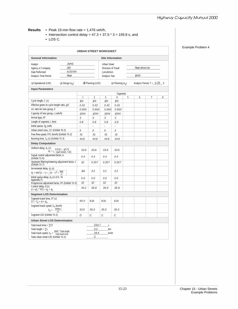
EXAMPLE PROBLEM 4

The Urban Street A 3.2-km divided four-lane urban street with four signalizedintersections at 0.8-km spacing. All intersections have left-turn bays.

The Question What are the LOS, control delay, and peak 15-min flow rate for thethrough volume?

The Facts√ FFS = 70 km/h, √ Urban street Class II,√ AADT = 30,000, √ Arrival Type 3,√ K = 0.091, D = 0.568, √ Actuated signal,√ PHF = 0.925, √ Cycle length = 120 s,√ s = 1,850 pc/h/ln, √ Average g/C = 0.42, and√ PLT = 0.12, √ Analysis period = 0.25 h.

Outline of Solution All input parameters are known for a planning application. Thethrough-volume peak 15-min flow rate, urban street speed, and LOS are computed.

Steps1. Find V. V = AADT * K * D

V = 30,000 * 0.091 * 0.568 = 1,551 veh/h

2. Find 15-min through flowrate. vp =

V (1 – PLT)PHF

vp = 1551 (1 – 0.12)

0.925 = 1,476 veh/h

3. Find c and X. c = s * N * (g/C)

c = 1850 * 2 * 0.42 = 1,554 pc/h

X = vc =

14761554 = 0.950

4. Find PF, k, and I (useExhibits 15-5, 15-6, and15-7).

PF = 1.0, k = 0.4. Assume I = 1.0 (for Intersection 1)and I = 0.207 is calculated for others

5. Find d1 (use Equation 15-2).d1 =

0.5(120)(1 – 0.42)2

1 – (0.42)(0.950) = 33.6 s

6. Find d2 (use Equation 15-3).d2 = 900(0.25) (0.950 − 1) + (0.950 − 1)2 +

8 *0.4*1.0*0.9501554(0.25)

d2 = 11.6 s

7. Find d (use Equation 15-1). d = (33.6 * 1.0) + 11.6 = 45.2 s

8. Find running time for asegment length of 800 m(use Exhibit 15-3).

Running time per km = 56 s/km

TR = 56 * 0.8 = 44.8 s

9. Find SA for a segment (useEquation 15-6a). SA =

3,600 0.8( )44.8 + 45.2( )

= 32.0 km/h, LOS D

10. Find SA for the entire urbanstreet (use Equation 15-6b). SA =

3,600 0.8 * 4( )334.7( )

= 34.4 km/h

11. Determine LOS (use Exhibit15-2).

LOS C


Results • Peak 15-min flow rate = 1,476 veh/h,• Intersection control delay = 47.3 + 37.5 * 3 = 159.8 s, and• LOS C.

Example Problem 4

Delay Computation









Input Parameters

Segments1 2 3 4 5 6 7 8

Cycle length, C (s)




Arrival type, AT







Total length = ∑L ________________km





SA =





d2 =



3600(L)ST

0.5C[(1 – g/C)2]1 – [(g/C)min(X, 1.0)]


900T (X – 1) + [(X – 1)2 + 8kIXcT

JMYECEI Peak direction5/20/99Peak 1999

0.25X

120 120 120 1200.42 0.42 0.42 0.420.950 0.950 0.950 0.9501,554 1,554 1,554 1,5543 3 3 30.8 0.8 0.8 0.8- - - -II II II II70 70 70 7044.8 44.8 44.8 44.8

33.6 33.6 33.6 33.6

0.4 0.4 0.4 0.4

1.0 0.207 0.207 0.207

11.6 3.2 3.2 3.2

0.0 0.0 0.0 0.0

1.0 1.0 1.0 1.0

45.2 36.8 36.8 36.8

90.0 81.6 81.6 81.6

32.0 35.3 35.3 35.3

D C C C

334.73.234.4C



EXAMPLE PROBLEM 5

The Urban Street A new 3.6-km six-lane facility with six signalized intersections at0.6-km spacing.

The Question What is the lowest acceptable travel speed, hourly directionalvolume, and annual average daily traffic to achieve LOS D?

The Facts√ FFS = 65 km/h, √ Urban street Class II,√ K = 0.095, D = 0.55, √ Arrival Type 5,√ PHF = 0.95, √ Semiactuated signals,√ s = 1,750 pc/h/ln, √ Cycle length = 120 s, and√ PLT = 0.12, √ g/C = 0.42.

√ Analysis period = 0.25 h,

Outline of Solution All input parameters are known. Find the lowest acceptable travelspeed to achieve LOS D, and backsolve for flow rate, volume, and AADT.

Steps

1. Find the lowest acceptabletravel speed for urban streetClass II and LOS D (useExhibit 15-2).

SA = 26.1 km/h

2. Find travel time for segmentlength of 600 m (use Exhibit15-3).

Running time per km = 61 s/kmTR = 61 * 0.6 = 36.6 s

Urban street travel time = 6 * 36.6 = 219.6 s

3. Find d for the total urbanstreet (use Equation 15-6).

d =3,600L

SA− TR

d =3,600(3.6)

26.1− 219.6 = 277.0 s/veh

4. Find PF, k, and I (useExhibits 15-5, 15-6, and15-7).

PF = 0.511, k = 0.4

Assume I = 1.0 (Intersection 1)

I = 0.090 is calculated for Intersections 2 through 6

5. Find c (use Equation 15-7). c = N * s * (g/C)

c = 3 * 1,750 * 0.42 = 2,205 veh/h

6. Find X (use Equations 15-1,15-2, and 15-3).

d = di1

6∑ = 277 s/veh

d = 6d1 * PF + d2 (Int. 1) + 5d2 (Int. 2–6)

d = 6 * 0.511 * d1 + d2 (Int. 1) + 5d2 (Int. 2–6)

d = 3.066d1 + d2 (Int. 1) + 5d2 (Int. 2–6)

d1 =0.5(120)(1− 0.42)2

1− 0.42 * min(1,X)

d1 =20.184

1− 0.42 * min(1,X)



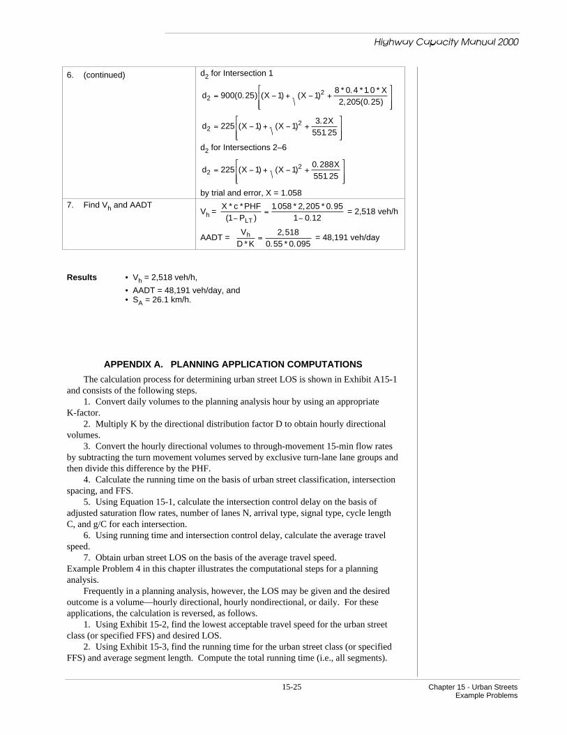
6. (continued) d2 for Intersection 1

d2 = 900(0.25) (X −1) + (X −1)2 +8 * 0.4 *1.0 * X2,205(0.25)

d2 = 225 (X −1) + (X −1)2 +3.2X

551.25

d2 for Intersections 2–6

d2 = 225 (X −1) + (X −1)2 +0.288X551.25

by trial and error, X = 1.0587. Find Vh and AADT

Vh = X * c *PHF(1−PLT )

=1.058 * 2,205 * 0.95

1− 0.12 = 2,518 veh/h

AADT = Vh

D * K=

2,5180.55 * 0.095

= 48,191 veh/day

Results • Vh = 2,518 veh/h,

• AADT = 48,191 veh/day, and• SA = 26.1 km/h.

APPENDIX A. PLANNING APPLICATION COMPUTATIONS

The calculation process for determining urban street LOS is shown in Exhibit A15-1and consists of the following steps.

1. Convert daily volumes to the planning analysis hour by using an appropriateK-factor.

2. Multiply K by the directional distribution factor D to obtain hourly directionalvolumes.

3. Convert the hourly directional volumes to through-movement 15-min flow ratesby subtracting the turn movement volumes served by exclusive turn-lane lane groups andthen divide this difference by the PHF.

4. Calculate the running time on the basis of urban street classification, intersectionspacing, and FFS.

5. Using Equation 15-1, calculate the intersection control delay on the basis ofadjusted saturation flow rates, number of lanes N, arrival type, signal type, cycle lengthC, and g/C for each intersection.

6. Using running time and intersection control delay, calculate the average travelspeed.

7. Obtain urban street LOS on the basis of the average travel speed.Example Problem 4 in this chapter illustrates the computational steps for a planninganalysis.

Frequently in a planning analysis, however, the LOS may be given and the desiredoutcome is a volume—hourly directional, hourly nondirectional, or daily. For theseapplications, the calculation is reversed, as follows.

1. Using Exhibit 15-2, find the lowest acceptable travel speed for the urban streetclass (or specified FFS) and desired LOS.

2. Using Exhibit 15-3, find the running time for the urban street class (or specifiedFFS) and average segment length. Compute the total running time (i.e., all segments).


Chapter 15 - Urban Streets 15-26Appendix A

EXHIBIT A15-1. URBAN STREET LOS CALCULATIONS

Running Time- Urban street class- Segment length- FFS- Exhibit 15-3

Intersection Total Delay- Adjusted saturation flow rate- Number of lanes- Arrival type- Signal type- Cycle length- Effective green time- Equations 15-1 through 15-3

Equation 15-6

Running Time and Intersection Total Delay Considerations

Time and Directional Considerations- Daily traffic volume- Planning analysis PHF- Two-way hourly volumes- Directional distribution factor- Hourly directional volume- Percent turns from exclusive lanes PHF- Basic through volume 15-min flow rate

LOS Considerations- Average travel speed- LOS criteria- LOS determination

3. Using Equation 15-6a and the values from Steps 1 and 2, calculate the controldelay d at the intersections.

4. Using Exhibit 15-4, find arrival type based on expected progression quality.Using Exhibit 15-5, find PF for specified green ratio and arrival type. Use a k-value of0.4. Use Exhibit 15-7 and an assumed value for Xu to find the I-value.

5. Use Equation 15-7 to compute capacity c of the through lane.6. Compute X by inserting the values from Steps 3 to 5 in Equations 15-1 through

15-3. Trial-and-error will be needed to reconcile delay from Step 3 with that predicted byEquation 15-1.

7. Use c from Step 5 and X from Step 6 with the percentage of turns from exclusivelanes and the PHF to determine the hourly directional volume Vh.

8. Use Vh from Step 7, the directional distribution factor D, and the K-factor tocalculate the AADT for the planning analysis hour.

The results of a planning analysis can range from a rough estimate of LOS to aprecise operational analysis, depending primarily on the extent to which default valuesare used as input. For example, using statewide defaults for appropriate traffic, roadway,and signal characteristics will produce rough LOS estimates. Using area- or roadway-specific data but treating all signal characteristics the same (e.g., using a weighted g/Capproach) should provide more accurate LOS estimates. However, using specific traffic,roadway, and signal data for each road segment and traffic signal would provide an evenmore accurate estimate. The next level of precision is a detailed treatment of turningmovements and signal timing, which approaches an operational analysis but usesprojected instead of actual traffic volumes.


15-27 Chapter 15 - Urban StreetsAppendix B

APPENDIX B. TRAVEL TIME STUDIES FOR DETERMINING LOS

The following steps apply the test-car method for determining travel time and LOSfor urban streets.

1. Identify and inventory the geometrics and the access control of each streetsegment, the segment lengths, the signal timing, and the 15-min flow rates for selectedtimes of the day—such as the peak a.m. period, the peak p.m. period, and a representativeoff-peak period—by direction of flow.

2. Determine the appropriate FFS for the street segment. This can be determined bymaking runs with a test car equipped with a calibrated speedometer during periods of lowvolume. An observer should read the speedometer at midblock locations when thevehicle is not impeded by other vehicles and record speed readings for each segment.These observations can be supplemented by spot speed studies at typical midblocklocations during low-volume conditions. Other data, such as design type, access points,roadside development, and speed limit, also may be considered.

3. Use Exhibits 10-3 and 10-4 along with the physical information and FFS todetermine the urban street class.

4. Make test-car travel time runs over the street segment during the selected times.a. Use the appropriate equipment to obtain the information identified in Exhibit

B15-1. The equipment may be computerized or simply a pair of stopwatches.b. Travel times between the centers of signalized intersections should be recorded,

along with the location, cause, and duration of each stop.c. Test-car runs should begin at different time points in the signal cycle to avoid all

trips starting first in the platoon.d. Some midblock speedometer readings also should be recorded to check on

unimpeded travel speeds and how they relate to FFS.e. Data should be summarized for each segment and each time period, the average

travel time, the average stopped time for the signal, and other stops and events (four-waystops, parking disruptions, etc.).

f. The number of test-car runs will depend on the variance in the data. Six to 12runs may be adequate for each traffic-volume condition.

g. If available, an instrumented test car should be used to reduce labor requirementsand to facilitate recording and analysis. Summaries of test-car runs with all data recordedand analyzed by the computer are now common.

5. The average travel speed, based on travel times and segment lengths, should bedetermined for each segment for each time period. Total travel speed for the urban streetshould also be determined.

6. From Exhibit 15-2, obtain a LOS value for each urban street segment and for theoverall urban street for each time period and direction of flow. This is done bycomparing the average travel speed from step 5 with the speed values for the appropriatestreet class in Exhibit 15-2.

7. The test-car data can be modified to evaluate different signal timing plans. Asshown in Exhibit 15-5, adjustment factors can be applied to delays to evaluate how thechanges would affect average travel speeds and LOS.



Chapter 15 - Urban Streets 15-28Appendix B

EXHIBIT B15-1. TRAVEL-TIME FIELD WORKSHEET

TRAVEL-TIME FIELD WORKSHEET

Analyst ___________________________ Urban Street _________________________

Agency or Company ___________________________ Direction of Travel _________________________

Date Performed ___________________________ Jurisdiction _________________________

Analysis Time Period ___________________________ Analysis Year _________________________


Field Data

Run No.__________ Run No. __________ Run No. __________

Time ____________ Time ____________ Time ____________

Signal Distance Cumulative Travel Delay Time Cumulative Travel Delay Time Cumulative Travel Delay Time Location (km) Time (s) (s) Time (s) (s) Time (s) (s)

APPENDIX C. WORKSHEETS



Chapter 15 - Urban Streets

Delay Computation









Input Parameters

Segments1 2 3 4 5 6 7 8

Cycle length, C (s)




Arrival type, AT







Total length = ∑L ________________km





SA =





d2 =


" Operational (LOS) " Design (vp) " Planning (LOS) " Planning (vp) Analysis Period, T =_______ h

3600(L)ST

0.5C[(1 – g/C)2]1 – [(g/C)min(X, 1.0)]


900T (X – 1) + [(X – 1)2 + 8kIXcT


Chapter 15 - Urban Streets



Analyst ___________________________ Urban Street __________________________

Agency or Company ___________________________ Direction of Travel __________________________

Date Performed ___________________________ Jurisdiction __________________________

Analysis Time Period ___________________________ Analysis Year __________________________


Field Data

Run No.__________ Run No. __________ Run No. __________

Time ____________ Time ____________ Time ____________

Signal Distance Cumulative Travel Delay Time Cumulative Travel Delay Time Cumulative Travel Delay Time Location (km) Time (s) (s) Time (s) (s) Time (s) (s)

ch15 urban streets - againc.net · highway capacity manual 2000 15-1 chapter 15 - urban streets...

Documents