ch05 finite element method-1d
DESCRIPTION
FEATRANSCRIPT

Piecewise Approximationand
Finite Element Method in 1D
Jayadeep U. B.
M.E.D., NIT Calicut
Ref.: Finite Elements and Approximation, Zienkiewicz, O. C., and Morgan, K., John Wiley & Sons.

2
Department of Mechanical Engineering, National Institute of Technology Calicut
Introduction
The trial functions can not be chosen easily, which are defined and with continuous derivatives over the complete domain.
Why Discretization?
Improving the accuracy necessitates increasing the number of trial functions used, leading to highly complex formulation of the problem.
The stiffness matrix obtained is generally complete (with non-zero elements at all positions) – Computational complexity.
Generally, it is tough to find functions satisfying the B.C. for complicated domains.
In F.E.M., the domain is discretized into a large number of sub-domains, each of which will have simple geometry.
Any trial function will have non-zero magnitude only over few adjacent sub-domains. The approx’ns over individual sub-domains can be added to get global approx’n.
Lecture - 01
3
Department of Mechanical Engineering, National Institute of Technology Calicut
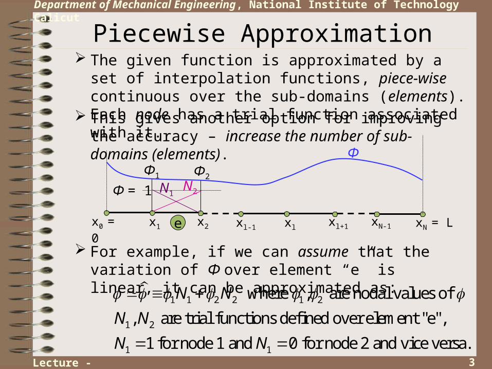
Piecewise Approximation The given function is approximated by a set of interpolation
functions, piece-wise continuous over the sub-domains (elements). Each node has a trial function associated with it.
This gives another option for improving the accuracy – increase the number of sub-domains (elements).
For example, if we can assume that the variation of Φ over element “e” is linear, it can be approximated as:
1 1 2 2 1 2
1 2
1 1
where , are nodal values of
, are trial functions defined over element "e",
1 for node 1 and 0 for node 2 and vice versa.
N N
N N
N N
x0 = 0 x1 x2 xl-1 xlxl+1 xN-1 xN = Le
Φ1 Φ2
N1N2Φ = 1
Φ
Lecture - 01
4
Department of Mechanical Engineering, National Institute of Technology Calicut
Piecewise Approximation contd. …
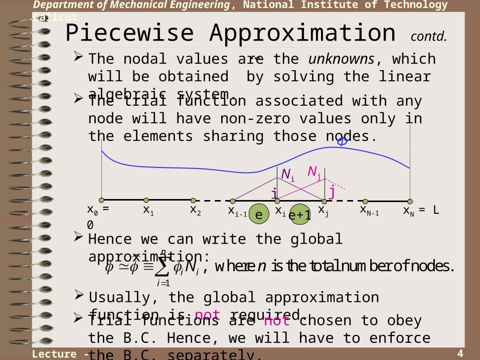
The nodal values are the unknowns, which will be obtained by solving the linear algebraic system.
The trial function associated with any node will have non-zero values only in the elements sharing those nodes.
Hence we can write the global approximation:
1
, where is the total number of nodes.n
i ii
N n
x0 = 0 x1 x2 xi-1 xixj xN-1 xN = Le
NiNj
Φ
e+1
i j
Usually, the global approximation function is not required.
Trial functions are not chosen to obey the B.C. Hence, we will have to enforce the B.C. separately.
Lecture - 01
5
Department of Mechanical Engineering, National Institute of Technology Calicut
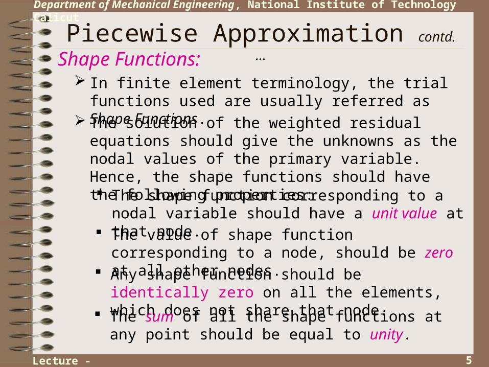
In finite element terminology, the trial functions used are usually referred as Shape Functions.
Shape Functions:
The solution of the weighted residual equations should give the unknowns as the nodal values of the primary variable. Hence, the shape functions should have the following properties: The shape function corresponding to a nodal variable
should have a unit value at that node. The value of shape function corresponding to a node,
should be zero at all other nodes. Any shape function should be identically zero on all the
elements, which does not share that node.
The sum of all the shape functions at any point should be equal to unity.
Piecewise Approximation contd. …
Lecture - 01
6
Department of Mechanical Engineering, National Institute of Technology Calicut
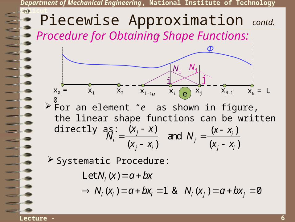
For an element “e” as shown in figure, the linear shape functions can be written directly as:
Procedure for Obtaining Shape Functions:Piecewise Approximation contd. …
x0 = 0 x1 x2 xl-1 xixj xN-1 xN = Le
NiNj
Φ
i j
( ) ( ) and
( ) ( )j i
i jj i j i
x x x xN N
x x x x
Systematic Procedure:
Let ( )
( ) 1 & ( ) 0i
i i i i j j
N x a bx
N x a bx N x a bx
Lecture - 01
7
Department of Mechanical Engineering, National Institute of Technology Calicut
Piecewise Approximation contd. …
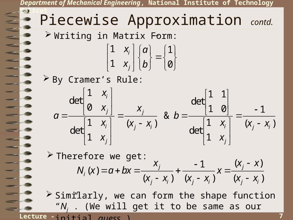
Writing in Matrix Form:
1 1
1 0i
j
x a
x b
By Cramer’s Rule:
1 1 1det det
0 1 0 1 &
1 1( ) ( )det det
1 1
i
j j
i ij i j i
j j
x
x xa b
x xx x x x
x x
Therefore we get:( )1
( )( ) ( ) ( )
j ji
j i j i j i
x x xN x a bx x
x x x x x x
Similarly, we can form the shape function “Nj”. (We will get it to be same as our initial guess.)
Lecture - 01
8
Department of Mechanical Engineering, National Institute of Technology Calicut
Piecewise Approximation contd. …
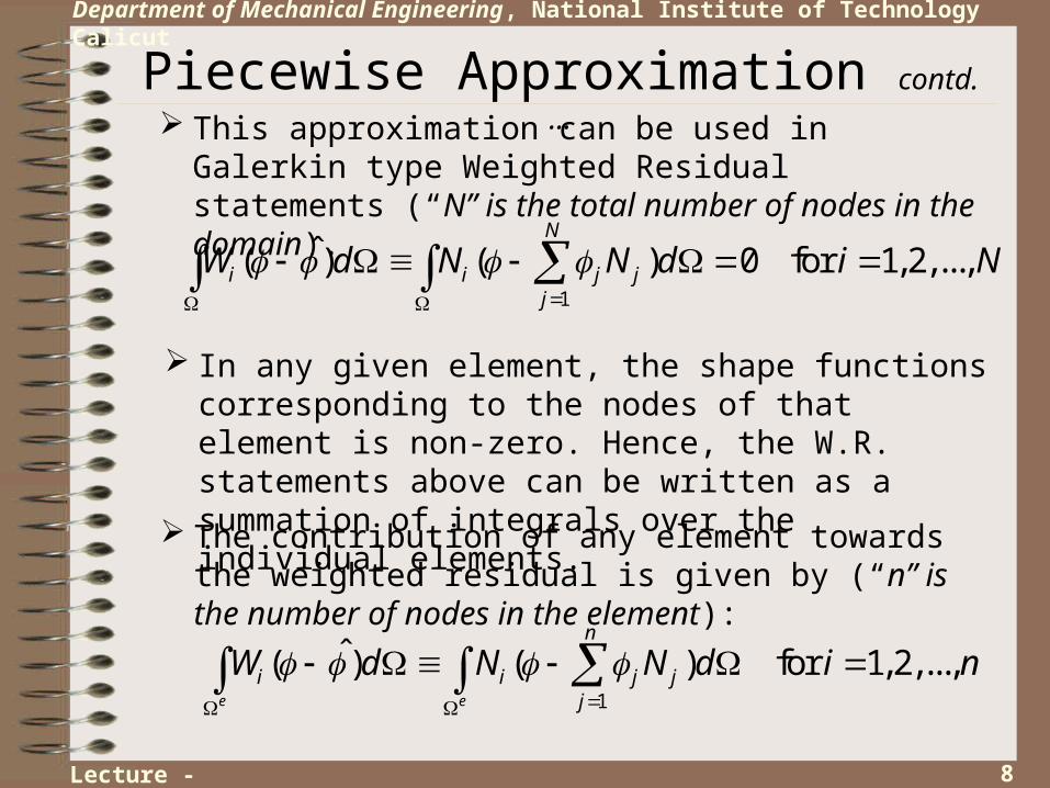
This approximation can be used in Galerkin type Weighted Residual statements (“N” is the total number of nodes in the domain).
In any given element, the shape functions corresponding to the nodes of that element is non-zero. Hence, the W.R. statements above can be written as a summation of integrals over the individual elements.
1
ˆ( ) ( ) 0 for 1,2,...,N
i i j jj
W d N N d i N
The contribution of any element towards the weighted residual is given by (“n” is the number of nodes in the element):
1
ˆ( ) ( ) for 1,2,...,e e
n
i i j jj
W d N N d i n
Lecture - 01
9
Department of Mechanical Engineering, National Institute of Technology Calicut
Piecewise Approximation contd. …
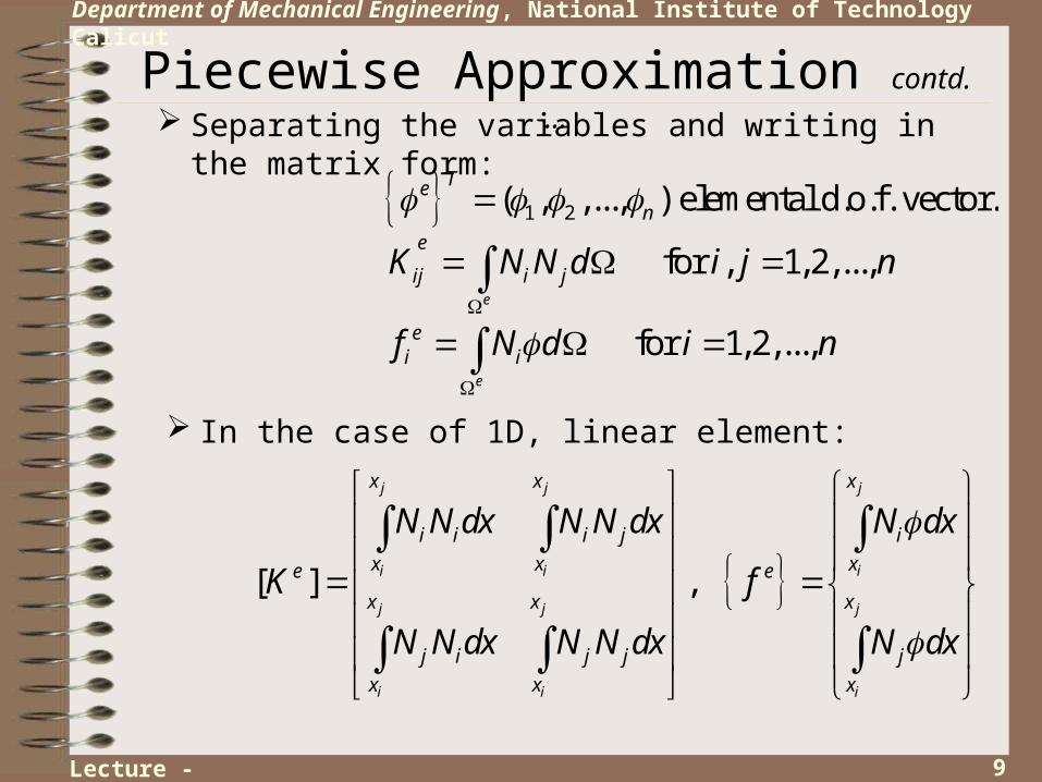
In the case of 1D, linear element:
[ ] ,
j j j
i i i
j j j
i i i
x x x
i i i j i
x x xe e
x x x
j i j j j
x x x
N N dx N N dx N dx
K f
N N dx N N dx N dx
Separating the variables and writing in the matrix form:
1 2( , ,..., ) elemental d.o.f. vector.
for , 1, 2,...,
for 1,2,...,
e
e
Ten
e
ij i j
ei i
K N N d i j n
f N d i n
Lecture - 01
10
Department of Mechanical Engineering, National Institute of Technology Calicut
Piecewise Approximation contd. …
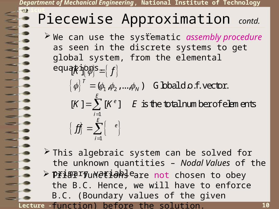
This algebraic system can be solved for the unknown quantities – Nodal Values of the primary variable.
We can use the systematic assembly procedure as seen in the discrete systems to get global system, from the elemental equations.
Trial functions are not chosen to obey the B.C. Hence, we will have to enforce B.C. (Boundary values of the given function) before the solution.
1 2
1
1
[ ]
( , ,..., ) Global d.o.f. vector.
[ ] [ ] is the total number of elements
T
NE
e
iE
e
i
K f
K K E
f f
Lecture - 01
11
Department of Mechanical Engineering, National Institute of Technology Calicut
Piecewise Approximation contd. …
Use 4 elements of equal length.
Home Work Problem: Approximate Φ(x) = sin(x), over the domain 0 ≤ x ≤ π, using piecewise defined linear interpolation functions.
Use Galerkin type Weighted Residual formulation, to find the nodal values.
Compare the approximation function values at π/6, π/3, 2π/3 and 5π/6 with the corresponding values of the given function.
Lecture - 01
12
Department of Mechanical Engineering, National Institute of Technology Calicut
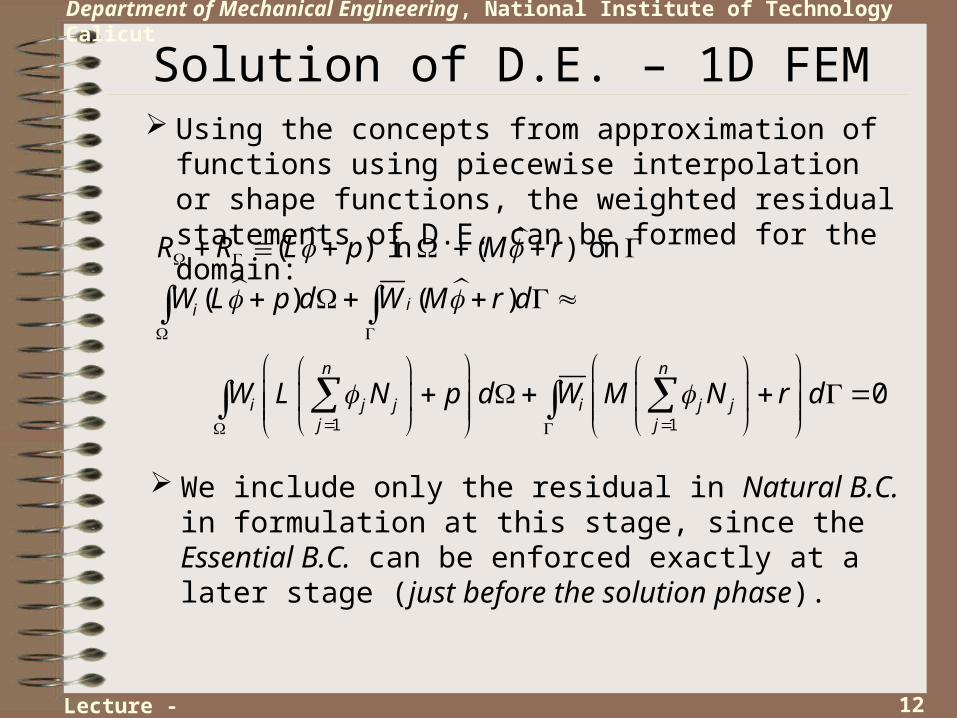
Solution of D.E. – 1D FEM Using the concepts from approximation of functions using
piecewise interpolation or shape functions, the weighted residual statements of D.E. can be formed for the domain:
We include only the residual in Natural B.C. in formulation at this stage, since the Essential B.C. can be enforced exactly at a later stage (just before the solution phase).
1 1
( ) in ( ) on
( ) ( )
0
ii
n n
i j j i j jj j
R R p r
W p d W r d
W N p d W N r d
L M
L M
L M
Lecture - 02
13
Department of Mechanical Engineering, National Institute of Technology Calicut
Solution of D.E. – 1D FEM contd. …
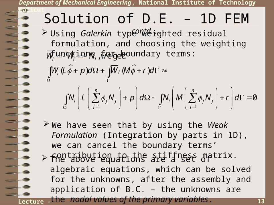
Using Galerkin type weighted residual formulation, and choosing the weighting functions for boundary terms:
We have seen that by using the Weak Formulation (Integration by parts in 1D), we can cancel the boundary terms’ contribution to the stiffness matrix.
The above equations are a set of algebraic equations, which can be solved for the unknowns, after the assembly and application of B.C. – the unknowns are the nodal values of the primary variables.
1 1
, we get:
( ) ( )
0
i i i
ii
n n
i j j i j jj j
W W N
W p d W r d
N N p d N N r d
L M
L M
Lecture - 02
14
Department of Mechanical Engineering, National Institute of Technology Calicut
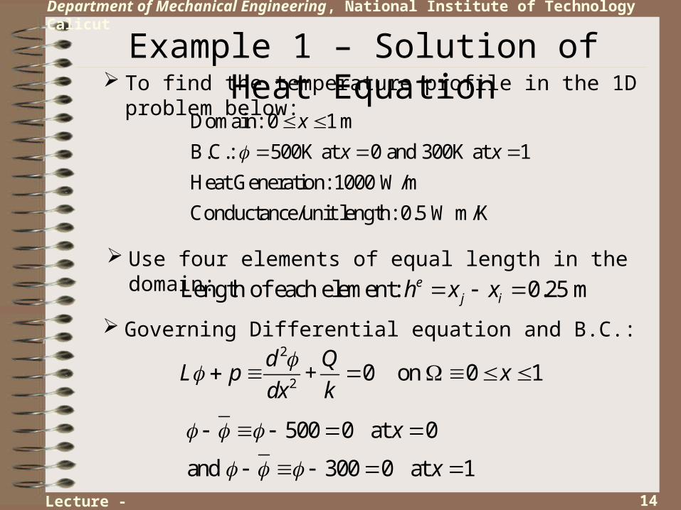
Example 1 – Solution of Heat Equation To find the temperature profile in the 1D problem below:
Use four elements of equal length in the domain:
Governing Differential equation and B.C.:
Domain: 0 1 m
B.C.: 500K at 0 and 300K at 1
Heat Generation: 1000 W/m
Conductance/unit length: 0.5 W m/K
x
x x
Length of each element: 0.25 mej ih x x
2
2+ 0 on 0 1
d Qp x
dx k
L
500 0 at 0
and 300 0 at 1
x
x
Lecture - 02

15
Department of Mechanical Engineering, National Institute of Technology Calicut
E.g. 1 – Solution of Heat Eq’n contd. …
Shape Functions (1D, Linear) for any element, with nodes “i” and “j”:
Domain discretization and numbering:
,j j i ii je e
j i j i
x x x x x x x xN N
x x h x x h
x1 = 0 x2 = 0.25 x3 = 0.5 x4 = 0.75 x5 = 11 2 3 4 51 2 3 4
N1 N2 N3 N4 N5
Lecture - 02

16
Department of Mechanical Engineering, National Institute of Technology Calicut
E.g. 1 – Solution of Heat Eq’n contd. …
Shape Functions (1D, Linear) for any element, with nodes “i” and “j”:
Galerkin WR Statements (considering the whole domain):
,j j i ii je e
j i j i
x x x x x x x xN N
x x h x x h
1 2
20
1 2
2j=10
+
+ 0 for 1,..., ,
where is the total number of nodes (= 5 here).
i i
M
i j j
d QN p dx N dx
dx k
d QN N dx i M
dx k
M
L
There is no residual at the boundary, since the Dirichlet or Essential B.C. specified in the problem can be exactly enforced, just before solving of the algebraic system.
Lecture - 02
17
Department of Mechanical Engineering, National Institute of Technology Calicut
E.g. 1 – Solution of Heat Eq’n contd. …
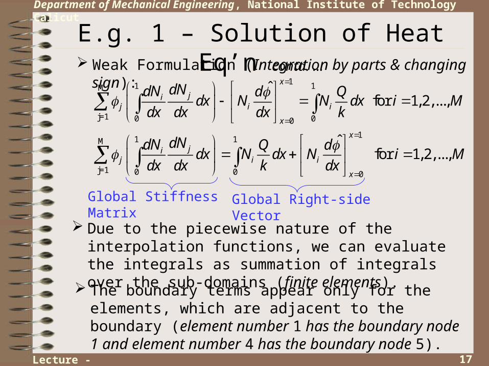
Weak Formulation (Integration by parts & changing sign):11 1M
j=1 0 00
11 1M
j=1 0 0 0
ˆ for 1, 2,...,
ˆ for 1, 2,...,
x
jij i i
x
x
jij i i
x
dNdN d Qdx N N dx i M
dx dx dx k
dNdN Q ddx N dx N i M
dx dx k dx
Due to the piecewise nature of the interpolation functions, we can evaluate the integrals as summation of integrals over the sub-domains (finite elements).
The boundary terms appear only for the elements, which are adjacent to the boundary (element number 1 has the boundary node 1 and element number 4 has the boundary node 5).
Global Stiffness Matrix Global Right-side Vector
Lecture - 02

18
Department of Mechanical Engineering, National Institute of Technology Calicut
E.g. 1 – Solution of Heat Eq’n contd. …
Over the element 1, with nodes 1 and 2:2 2
1 1 1
1 1ˆ
,x x
jiij i i i
x x x x
dNdN Q dK dx f N dx N
dx dx k dx
The shape function N1 corresponds to node 1 (x=x1=0) & N2 corresponds to node 2 (x=x2). Therefore the boundary term above is non-zero only when i=1. Further, N1=1 at x=x1.
All the elemental contributions can be added to get the global system, which corresponds to the original W.R. statements over the domain.
An assembly procedure, similar to that used in the discrete systems, needs to be followed, to ensure that the elemental contributions to the W.R. statements are properly added.
Lecture - 02

19
Department of Mechanical Engineering, National Institute of Technology Calicut
E.g. 1 – Solution of Heat Eq’n contd. …
In the Matrix form:
2 2
1 1
2 2
1 1
2
1 1
2
1
2
1 1 2
1
2
2 1 2
1
1
2
,
ˆ
x x
x x
x x
x x
x
x x x
x
x
dN dN dNdx dx
dx dx dxK
dN dN dNdx dx
dx dx dx
Q dN dx
k dxf
QN dx
k
Lecture - 02
20
Department of Mechanical Engineering, National Institute of Technology Calicut
E.g. 1 – Solution of Heat Eq’n contd. …
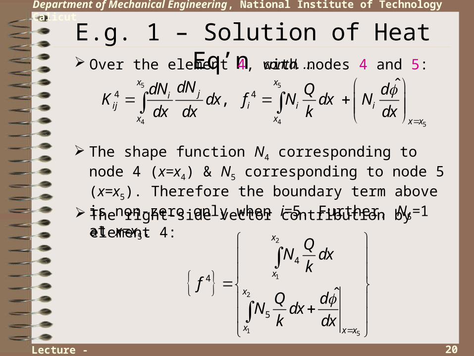
Over the element 4, with nodes 4 and 5:5 5
4 4 5
4 4ˆ
, x x
jiij i i i
x x x x
dNdN Q dK dx f N dx N
dx dx k dx
The shape function N4 corresponding to node 4 (x=x4) & N5 corresponding to node 5 (x=x5). Therefore the boundary term above is non-zero only when i=5. Further, N5=1 at x=x5.
The right-side vector contribution by element 4:
2
1
2
1 5
4
4
5
ˆ
x
x
x
x x x
QN dx
kf
Q dN dx
k dx
Lecture - 02
21
Department of Mechanical Engineering, National Institute of Technology Calicut
E.g. 1 – Solution of Heat Eq’n contd. …
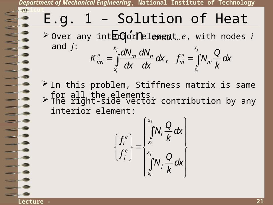
Over any interior element e, with nodes i and j:
,j j
i i
x x
e em nmn m m
x x
dN dN QK dx f N dx
dx dx k
In this problem, Stiffness matrix is same for all the elements.
j
i
j
i
x
iexi
e xj
j
x
QN dx
kf
f QN dx
k
The right-side vector contribution by any interior element:
Lecture - 02
22
Department of Mechanical Engineering, National Institute of Technology Calicut
E.g. 1 – Solution of Heat Eq’n contd. …
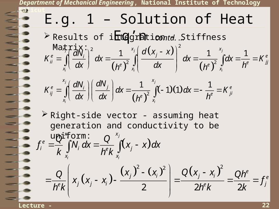
Results of integration - Stiffness Matrix:
22
2 2
2
1 1 1
1 11 1
j j j
i i i
j j
i i
x x xje ei
ii jjee ex x x
x x
je eiij jiee
x x
d x xdNK dx dx dx K
dx dx hh h
dNdNK dx dx K
dx dx hh
Right-side vector - assuming heat generation and conductivity to be uniform:
2 22
2 2 2
j j
i i
x x
ei i je
x x
ej i j i e
j j i je e
Q Qf N dx x x dx
k h k
x x Q x xQ Qhx x x f
h k h k k
Lecture - 02

23
Department of Mechanical Engineering, National Institute of Technology Calicut
E.g. 1 – Solution of Heat Eq’n contd. …
Writing in Matrix form, the elemental contribution for any interior element is:
1 1
2,1 1
2
e
e ee e
e
e e
Qh
h hK k fQh
h h
Substituting the values:
4 4 2 20.5
4 4 2 2
125&
125
e
e
K
f
The stiffness matrix will be same for element 1 & 4, but the right-side vector will have additional terms (for nodes 1 & 5)
We have to assemble these elemental contributions to obtain a global system.
Lecture - 02
24
Department of Mechanical Engineering, National Institute of Technology Calicut
E.g. 1 – Solution of Heat Eq’n contd. …
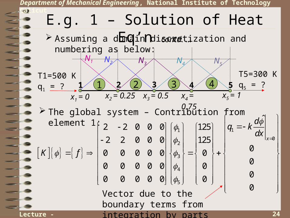
Assuming a domain discretization and numbering as below:
The global system – Contribution from element 1:
11
02
3
4
5
ˆ2 2 0 0 0 125
2 2 0 0 0 12500 0 0 0 0 000 0 0 0 0 000 0 0 0 0 00
x
dq k
dx
K f
Vector due to the boundary terms from integration by parts
x1 = 0 x2 = 0.25 x3 = 0.5 x4 = 0.75 x5 = 11 2 3 4 51 2 3 4
N1 N2 N3 N4 N5
T1=500 Kq1 = ?
T5=300 Kq5 = ?
Lecture - 02

25
Department of Mechanical Engineering, National Institute of Technology Calicut
E.g. 1 – Solution of Heat Eq’n contd. …
Adding the Contribution from element 2:
1 1
2
3
2 2 0 0 0 125
2 4 2 0 0 250
0 2 2 0 0 125
0 0 0 0 0 0 0
0 0 0 0 0 0 0
q
K f
Adding the Contributions from element 3 & 4, the global system:
1 1
2
3
4
5 5
1252 2 0 0 0
2502 4 2 0 0
2500 2 4 2 0
2500 0 2 4 2
1250 0 0 2 2
q
K f
q
Lecture - 02
26
Department of Mechanical Engineering, National Institute of Technology Calicut
E.g. 1 – Solution of Heat Eq’n contd. …
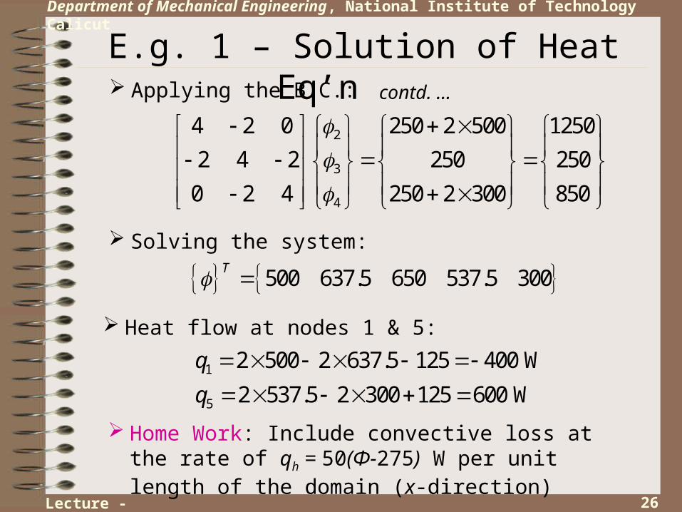
Applying the B.C.:
2
3
4
4 2 0 250 2 500 1250
2 4 2 250 250
0 2 4 250 2 300 850
Solving the system:
500 637.5 650 537.5 300T
Heat flow at nodes 1 & 5:
1
5
2 500 2 637.5 125 400 W
2 537.5 2 300 125 600 W
q
q
Home Work: Include convective loss at the rate of qh = 50(Φ-275) W per unit length of the domain (x-direction)
Lecture - 02

27
Department of Mechanical Engineering, National Institute of Technology Calicut
Higher Order Elements In the previous example, we assumed that any function can be
approximated using piecewise linear shape functions, provided a sufficient number of elements are used.
If we want to increase the accuracy, we have the option of increasing the number of elements (reducing the size).
However, it is intuitively obvious that we can get higher accuracy with the same mesh, if we use quadratic or higher order polynomials as shape functions.
The finite elements, which are based on such higher order shape functions are called higher order elements.
Lecture - 03
28
Department of Mechanical Engineering, National Institute of Technology Calicut
1D Second Order Elements We can use a similar procedure as earlier to get a quadratic
element – the fundamental properties of shape functions are quite general and should be satisfied in this case also.
To represent any general second order polynomial, we need to have three trial functions (3 nodes per element).
Hence, if we attach a shape function with a node, we need to have three nodes per element. In case of 1D, one of this node has to be internal to the element, while the other two form the inter-element boundary.
The internal node is generally placed midway between the end-nodes and therefore called the mid-side node.
There are cases, where the internal nodes are placed at locations other than mid-point. Examples are quarter point elements used in fracture mechanics applications (Another topic for Term Paper).
Lecture - 03
29
Department of Mechanical Engineering, National Institute of Technology Calicut
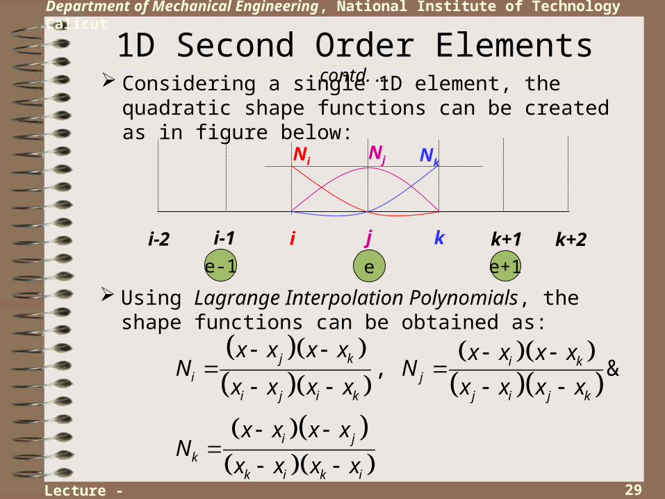
1D Second Order Elements contd. …
Considering a single 1D element, the quadratic shape functions can be created as in figure below:
Using Lagrange Interpolation Polynomials, the shape functions can be obtained as:
, &j k i k
i j
i j i k j i j k
i j
kk i k i
x x x x x x x xN N
x x x x x x x x
x x x xN
x x x x
i kj
ee-1 e+1
i-1i-2 k+1 k+2
NiNj Nk
Lecture - 03
30
Department of Mechanical Engineering, National Institute of Technology Calicut
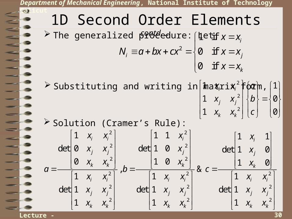
1D Second Order Elements contd. …
The generalized procedure: Let,2
1 if
0 if
0 if
i
i j
k
x x
N a bx cx x x
x x
Substituting and writing in matrix form, 2
2
2
1 1
1 0
1 0
i i
j j
k k
x x a
x x b
x x c
Solution (Cramer’s Rule):
2 2
2 2
2 2
2 2 2
2 2 2
2 2 2
1 1 1 1 1det 0 det 1 0 det 1 0
0 1 0 1 0, &
1 1 1
det 1 det 1 det 1
1 1 1
i i i i
j j j j
k k k k
i i i i i i
j j j j j j
k k k k k k
x x x xx x x xx x x x
a b cx x x x x x
x x x x x x
x x x x x x
Lecture - 03

31
Department of Mechanical Engineering, National Institute of Technology Calicut
1D Second Order Elements contd. …
Verify that we get the same expressions for the shape functions as we guessed initially.
Whether the sum of all the shape functions at any point inside the element is unity?
We can extend the same methodology for creating cubic or even higher order shape functions. A 1D cubic element should have 4 nodes – 2 end-nodes and 2 internal nodes. What should be the position of internal nodes?
Interpolation (trial) functions of any order for C0 continuous elements can be generated using Lagrange Interpolation Polynomials and hence these are called Lagrangian Family of finite elements.
Lecture - 03
We can use functions other than the polynomials as shape functions. For example, the harmonic shape functions used in axisymmetric elements with non-axisymmetric loads (Another topic for Term Paper).

32
Department of Mechanical Engineering, National Institute of Technology Calicut
Continuity of Shape Functions
Consider the case of finding the solution of D.E. subject to certain B.C. as earlier. Writing the W.R. statement:
In the previous problem, we have assumed the field variable to be continuous everywhere, while the derivatives are continuous only within the element.
1 1
( ) in ( ) on
( ) ( )
0
ii
n n
i j j i j jj j
R R p r
W p d W r d
W N p d W N r d
L M
L M
L M
What order of continuity is required for the shape functions?
The significant question is, what order of continuity we need to ensure for the shape functions, to solve a general D.E.?
Lecture - 04

33
Department of Mechanical Engineering, National Institute of Technology Calicut
Continuity of Shape Functions contd. …
Let us consider the inter-element continuity (near junction A), of three types of shape functions:
Nm
A
dNm/dx
A
∞dNm/dx
A
d2Nm/dx2
A
∞
Nm
A
d2Nm/dx2
A
d3Nm/dx3
A
∞
dNm/dx
A
Nm
A
Lecture - 04
34
Department of Mechanical Engineering, National Institute of Technology Calicut
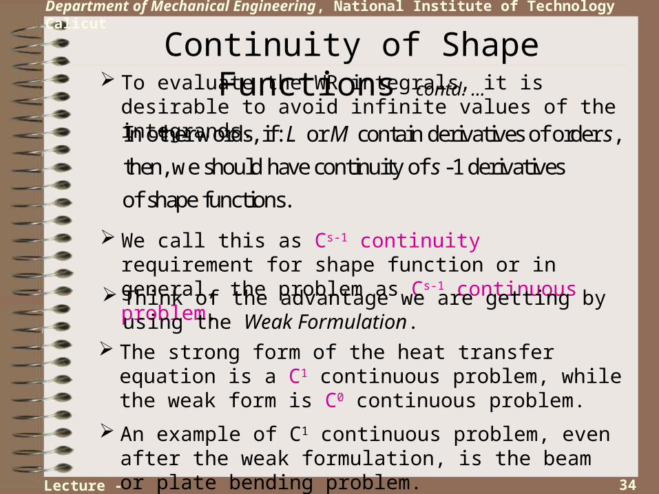
Continuity of Shape Functions contd. …
To evaluate the WR integrals, it is desirable to avoid infinite values of the integrands.
We call this as Cs-1 continuity requirement for shape function or in general, the problem as Cs-1 continuous problem.
In other words, if: or contain derivatives of order ,
then, we should have continuity of -1 derivatives
of shape functions.
s
s
L M
Think of the advantage we are getting by using the Weak Formulation.
The strong form of the heat transfer equation is a C1 continuous problem, while the weak form is C0 continuous problem.
An example of C1 continuous problem, even after the weak formulation, is the beam or plate bending problem.
Lecture - 04
35
Department of Mechanical Engineering, National Institute of Technology Calicut
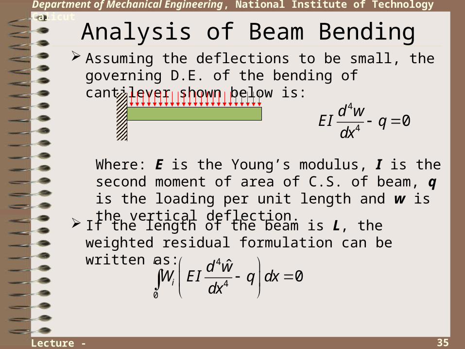
Analysis of Beam Bending Assuming the deflections to be small, the governing D.E. of
the bending of cantilever shown below is:
4
40
d wEI q
dx
Where: E is the Young’s modulus, I is the second moment of area of C.S. of beam, q is the loading per unit length and w is the vertical deflection.
If the length of the beam is L, the weighted residual formulation can be written as:
Lecture - 04
4
40
ˆ0
L
i
d wW EI q dx
dx

36
Department of Mechanical Engineering, National Institute of Technology Calicut
Analysis of Beam Bending contd.…
Integrating by parts:
3 3
3 30 00
ˆ ˆ0
L L Li
i i
dWd w d wW EI EI dx W qdx
dx dx dx
Integrating by parts again to obtain the weak form:
Lecture - 04
23 2 2
3 2 2 20 00 0
ˆ ˆ ˆ0
L L L Li i
i i
dW d Wd w d w d wW EI EI EI dx W qdx
dx dx dx dx dx
Second order derivatives appear even in the weak form.
Hence to avoid infinite values, the inter-element continuity of first order derivatives should be ensured.
Further, for the convenience of applying B.C.’s etc., the slope also is made as a primary variable, along with the deflection. Hence, there are two d.o.f. per node.
37
Department of Mechanical Engineering, National Institute of Technology Calicut
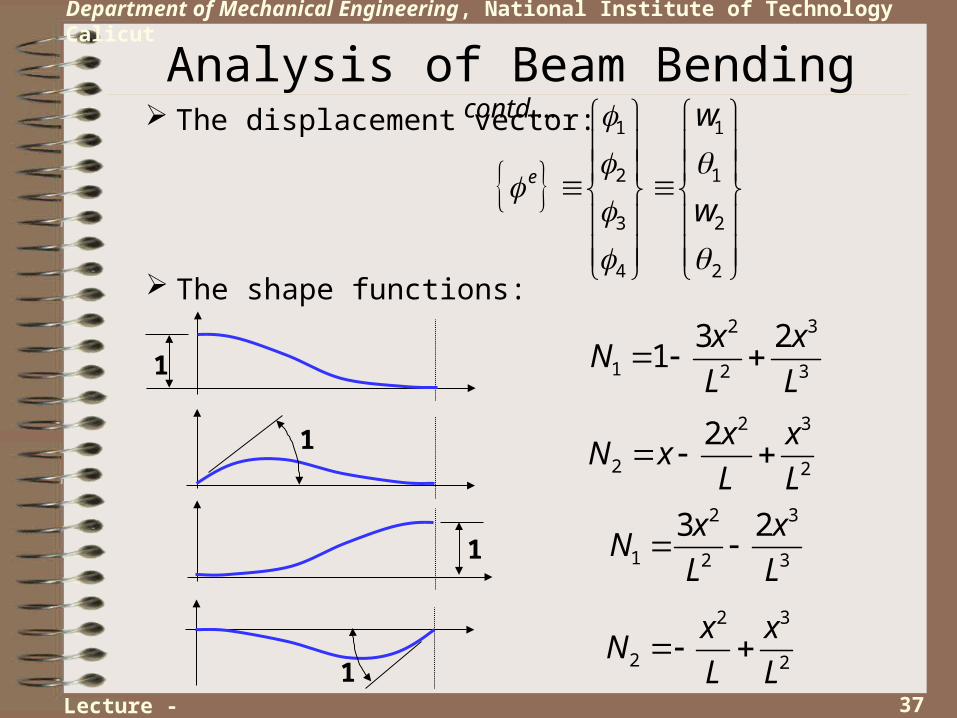
Analysis of Beam Bending contd.…
The displacement vector:
1 1
2 1
3 2
4 2
e
w
w
The shape functions:
Lecture - 04
2 3
1 2 3
3 21
x xN
L L
2 3
2 2
2x xN x
L L
1
1
2 3
1 2 3
3 2x xN
L L
2 3
2 2
x xN
L L
1
1
38
Department of Mechanical Engineering, National Institute of Technology Calicut
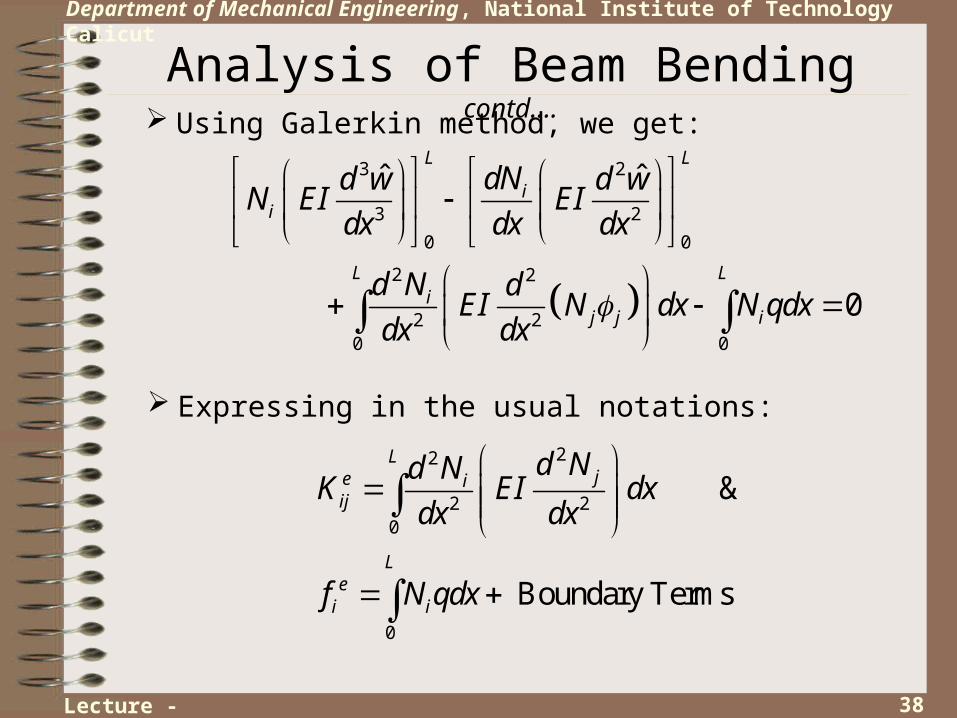
Analysis of Beam Bending contd.…
Using Galerkin method, we get:
Lecture - 04
3 2
3 2
0 0
2 2
2 20 0
ˆ ˆ
0
L L
ii
L Li
j j i
dNd w d wN EI EI
dx dx dx
d N dEI N dx N qdx
dx dx
Expressing in the usual notations:
22
2 20
0
&
Boundary Terms
Lje i
ij
Le
i i
d Nd NK EI dx
dx dx
f N qdx
39
Department of Mechanical Engineering, National Institute of Technology Calicut
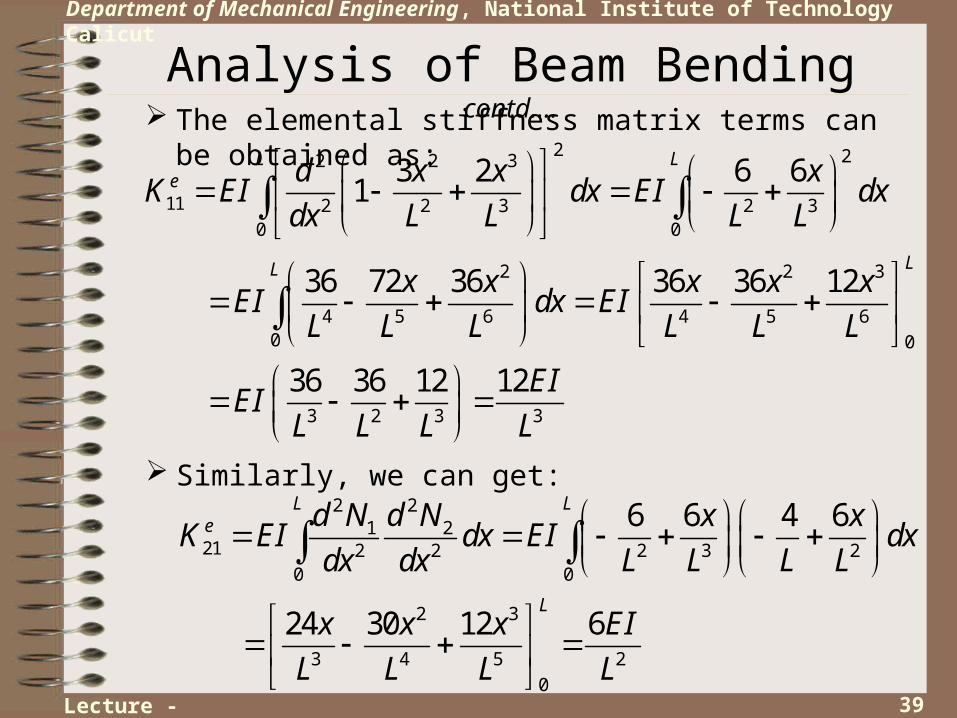
Analysis of Beam Bending contd.…
The elemental stiffness matrix terms can be obtained as:2 22 2 3
11 2 2 3 2 30 0
2 2 3
4 5 6 4 5 60 0
3 2 3 3
3 2 6 61
36 72 36 36 36 12
36 36 12 12
L Le
LL
d x x xK EI dx EI dx
dx L L L L
x x x x xEI dx EI
L L L L L L
EIEI
L L L L
Similarly, we can get:
Lecture - 04
2 21 2
21 2 2 2 3 20 0
2 3
3 4 5 2
0
6 6 4 6
24 30 12 6
L Le
L
d N d N x xK EI dx EI dx
dx dx L L L L
x x x EI
L L L L
40
Department of Mechanical Engineering, National Institute of Technology Calicut
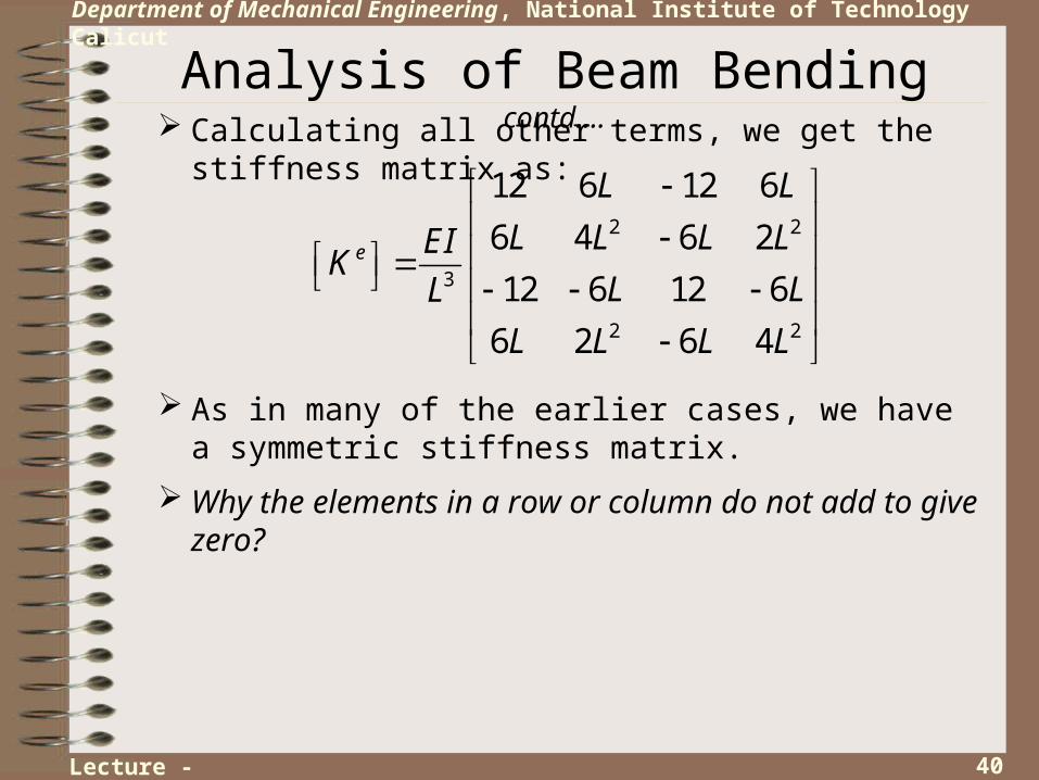
Analysis of Beam Bending contd.…
Calculating all other terms, we get the stiffness matrix as:
2 2
3
2 2
12 6 12 6
6 4 6 2
12 6 12 6
6 2 6 4
e
L L
L L L LEIK
L LL
L L L L
As in many of the earlier cases, we have a symmetric stiffness matrix.
Lecture - 04
Why the elements in a row or column do not add to give zero?
41
Department of Mechanical Engineering, National Institute of Technology Calicut
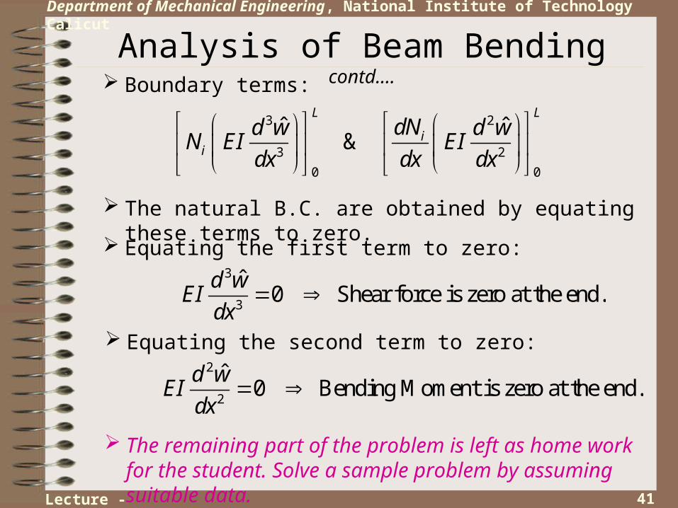
Analysis of Beam Bending contd.…
Boundary terms:
3 2
3 2
0 0
ˆ ˆ&
L L
ii
dNd w d wN EI EI
dx dx dx
The natural B.C. are obtained by equating these terms to zero.
Lecture - 04
Equating the first term to zero:3
3
ˆ0 Shear force is zero at the end.
d wEI
dx
Equating the second term to zero:2
2
ˆ0 Bending Moment is zero at the end.
d wEI
dx
The remaining part of the problem is left as home work for the student. Solve a sample problem by assuming suitable data.
42
Department of Mechanical Engineering, National Institute of Technology Calicut
Concluding Remarks In this chapter we developed the fundamental idea of FEM,
i.e., Piecewise defined trial functions, after discretizing the domain into finite elements.
We first applied this concept to approximation of known functions and then for the solution of differential equations, both in 1D.
Lecture - 04
By specifying the properties of the trial functions, we could directly solve for the nodal values of the unknown variable and obtain the global stiffness matrix to be sparse.
We discussed the idea of higher order trial functions (elements) and the continuity requirements.
However, all these discussions were limited to 1D, were the geometry is trivial. The real power of FEM appears in 2D or 3D problems, were simultaneous approximation of the field variable and the geometry is required.